Abstract
Air pollution in Macau has become a serious problem following the Pearl River Delta’s (PRD) rapid industrialization that began in the 1990s. With this in mind, Macau needs an air quality forecast system that accurately predicts pollutant concentration during the occurrence of pollution episodes to warn the public ahead of time. Five different state-of-the-art machine learning (ML) algorithms were applied to create predictive models to forecast PM2.5, PM10, and CO concentrations for the next 24 and 48 h, which included artificial neural networks (ANN), random forest (RF), extreme gradient boosting (XGBoost), support vector machine (SVM), and multiple linear regression (MLR), to determine the best ML algorithms for the respective pollutants and time scale. The diurnal measurements of air quality data in Macau from 2016 to 2021 were obtained for this work. The 2020 and 2021 datasets were used for model testing, while the four-year data before 2020 and 2021 were used to build and train the ML models. Results show that the ANN, RF, XGBoost, SVM, and MLR models were able to provide good performance in building up a 24-h forecast with a higher coefficient of determination (R2) and lower root mean square error (RMSE), mean absolute error (MAE), and biases (BIAS). Meanwhile, all the ML models in the 48-h forecasting performance were satisfactory enough to be accepted as a two-day continuous forecast even if the R2 value was lower than the 24-h forecast. The 48-h forecasting model could be further improved by proper feature selection based on the 24-h dataset, using the Shapley Additive Explanations (SHAP) value test and the adjusted R2 value of the 48-h forecasting model. In conclusion, the above five ML algorithms were able to successfully forecast the 24 and 48 h of pollutant concentration in Macau, with the RF and SVM models performing the best in the prediction of PM2.5 and PM10, and CO in both 24 and 48-h forecasts.
1. Introduction
The concentration of air pollutants is significantly influenced by different meteorological variables. These include atmospheric pressure, temperature, humidity, solar radiation, wind direction, and wind speed, which are factors for the movement of gases and aerosols to different heights, latitudes, and longitudes within a certain distance. In addition, the local air quality in Macau is also affected by the seasonal north and south monsoon, which brings transboundary pollutants from industrialized areas within the PRD. In Macau, local sources of emissions are from combustion activities, which include the burning of fossil fuels, industrial combustion, and waste incineration, as well as construction-related activities. Studies using statistical and ML methods have been carried out previously in Macau with promising results [1,2]. Vehicle emissions are a major source of the primary pollutants PM, CO, NO2, and SO2 [3]. The construction of infrastructure in Macau is also a significant source of PM2.5 and PM10 [4].
In winter, the northern monsoon brings transboundary pollutants such as PM2.5, and gases (SO2, NO2, and CO) from neighboring cities, which bring thick smog, reducing visibility and affecting human health [5,6]. The southwest monsoon brings frequent and sometimes heavy rainfall. It can effectively stop the spread of air pollutants from the north due to the change in wind direction and the amount of rainfall. Spring and autumn are relatively short transition periods [7]. The health impacts of air pollution were identified by several studies carried out by the WHO, and experts estimated that air pollution caused around 7 to 8 million deaths per year [8].
The air pollutants that affected Macau include PM2.5, PM10, NO2, and O3, similar to other modernized cities in Guangdong province [9]. Cardiovascular and respiratory diseases are the common causes of death in industrial locations, with air pollution caused by high levels of NO2, PM2.5, and PM10 concentration [10]. PM10 and PM2.5 are inhalable due to their small size, which may enter the human respiratory system through the nasal passages to the alveoli in the lung, and also by transfer to cellular tissues and the circulatory system [11,12,13]. Studies found that low levels of CO may exacerbate diseases such as angina and have other subtle chronic effects, while prolonged exposure (days–months) to low concentrations of CO may have subtle effects on the brain [14,15]. Macau has a high-density ratio of pollutant emission sources per km2 and also suffers from the effects of the long-range transport of PM2.5 to Macau by the northern monsoon [16,17].
Chemical transport models (CTM) are commonly used methods to forecast air quality accurately, but it usually takes a huge amount of calculation time and with large uncertainties [18]. ML models are one way to predict air quality in a fast and accurate way. Studies showed that the ANN model performed much better than the MLR model in predicting the PM10 concentration in Athens, Greece. It also outperformed MLR based on the same input parameters, along with a selection of algorithms to predict NO2 concentrations, in Auckland, New Zealand. Moreover, it performed well in the prediction of six air pollutants, including O3, NO2, PM10, PM2.5, SO2, and CO, and the AQI, in Ahvaz, Iran [19,20,21]. Other studies found that the LSTM model performed the best amongst MLR and ANN models and was able to predict high levels of PM2.5 concentration in Melbourne, Australia [22]. Also, SVM, with Pearson VII Universal Kernel (PUK), gave the highest R2 in the prediction of six air pollutants, and with the Radial Basis Function (RBF) Kernel, successfully predicted the AQI in New Delhi, India [23,24]. The RF model performed the best among DTR and ANN models in the prediction of AQI levels in Shenyang, China and performed well in the prediction of AQI in Beijing, China [25,26]. In addition, the XGBoost model outperformed RF, SVM, MLR, and DTR models, with high accuracy and low over-fitting probability, in the prediction of PM2.5 concentration in Tianjin, China [27]. Additionally, the use of CART and MLR has successfully predicted NO2, PM2.5, PM10, and O3 concentrations in Portugal and Macau, and RF performed the best amongst GB, SVM, and MLR models in the prediction of PM2.5 and PM10 in Macau [1,2]. Overall, these studies show that the ML methods perform well in air quality forecasts.
Before this study, there were no forecasting models that could accurately predict 48 h ahead of the air quality forecast in Macau. The models were developed to predict the 24 and 48-h concentrations of PM10, PM2.5, and CO for Taipa Ambient, Macau. This paper aims to determine the best ML methods, including ANN, RF, XGBoost, SVM, and MLR models to forecast air quality in Macau during air pollution episodes. It is expected that these ML algorithms are capable of performing air quality forecasts. This study may be used as a reference for neighboring cities and regions with similar geographical settings as Macau.
2. Materials and Methods
2.1. Data Acquisition
The work collected daily measurements of air quality data and meteorological parameters from the Macau Meteorological and Geophysical Bureau (SMG) and the Hong Kong Observatory (HKO) from 2016 to 2021 to build and train the ML models, using the features which are shown in Table 1 and are split into two categories. The first category is the time series data of air pollutant concentrations, including PM2.5, PM10, and CO from the previous days (D1, D2, D3) and 16D1 (from 1600 h yesterday to 1500 h today), because daily commutes may contribute disproportionately to overall daily exposure to urban air pollutants such as PM and CO [28]. The second category is the meteorological variables, subdivided into two groups—upper air observation and ground surface observation. Upper air observation variables indicate atmospheric stability versus trends and how atmospheric conditions influence the spread of pollutants within a certain area. The upper air observation data was collected from the Hong Kong Observatory’s King’s Park Station (45004) at 1200 h UTC every day as this is the closest World Meteorological Organization (WMO) recognized upper air observatory to Macau. Ground surface observation indicates trends regarding the capacity of air pollutant dispersion by wind and the deposition and removal of air pollutants by precipitation. These air quality forecast models are developed using the air quality variables and meteorological variables as the predictors of the study and applied to five different ML algorithms. With these big data collected over the years, the application of ML algorithms is possible to establish a training and testing dataset and extract important information from them.

Table 1.
Air quality forecasting variables considered as predictors for the ML models.
2.2. Procedure of Study
Figure 1 illustrates the workflow of this work, starting with the acquisition of data and data normalization for all the ML models. Once data preprocessing was completed, ANN, RF, XGBoost, SVM, and MLR models of the 24-h forecast were built, and hyperparameters were specifically tuned to ensure optimum performance. SHAP analysis was applied to analyze the 24-h forecasting model of each air pollutant, and each pollutant’s most dominant factors were identified. For the 48-h forecast, data normalization was required to re-identify the features’ time interval by adding 24 h. Afterwards, the data preprocessing started to build the primary 48-h model. Once it was built, the feature selection was required to enhance the model accuracy if the R2 was below 0.5 (defined threshold). The feature selection criteria are based on SHAP values and the characteristic of each meteorological feature. The highest adjusted R2 value determined the best feature-reduced model, and it must also be better than the R2 of the MLR model. For the 24-h best ML model, the adjusted R2 values were compared to analyze the influence of meteorological parameters in the ML models and the accuracy in combination, with and without, meteorological parameters. Lastly, the result of 24-h predictions for different years was compared and analyzed.
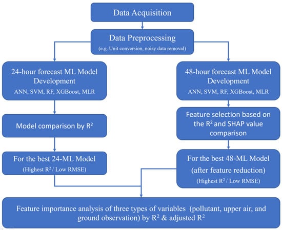
Figure 1.
The workflow of this study to develop the air quality forecast model for Macau.
2.3. Learning Algorithms
The ANN model consists of a network of neurons made of three parts: the input, the hidden, and the output layer, and when it is of suitable configuration and sufficient data is available, it can be used to fit any linear and non-linear functions [20].
The SVM model can accurately map, classify and fit the input data to a high dimensional space through a kernel function, and after mapping through the kernel function, the sample points can be separated by a hyperplane [29]. Mathematically, the SVM model can be described by the equation (Equation (1)),
where is the kernel function for high-dimensional mapping of the original data.
The RF model is an integrated learning model composed of multiple decision trees, each decision tree comprising three parts: the root, the leaf, and the internal node. The root node stores all the datasets, the internal node is used to classify the features, and the leaf node represents the different corresponding output results [30].
The XGBoost model is an extreme gradient boosting algorithm and a decision tree-based ensemble learning model with the core idea to fit and learn the residuals of the previous tree, with the final prediction result being the sum of the effects of all regression trees [31].
The objective function is shown by the following equation.
where is the measured value; is the predicted value of each tree; is the loss function, which is used to measure the total prediction error; is the regularization term, and is related to the structural complexity of each tree. It is added to the objective function to prevent overfitting caused by too strong a fitting ability.
The MLR model is an improved simple linear regression (SLR) that uses more than one independent variable to determine the linear relationship, with inputted data fitted to a hyperplane, which is generally a straight line in a high-dimensional space [19].
The regression equation of MLR is shown as follows:
where is the prediction value, is the independent variable, is the weight of variable, is the intercept, and is the error of the regression line.
SHAP value is a technique used to determine the contribution of each variable in the forecasting models, which was introduced in cooperative game theory, and obtained by calculating the marginal contribution of each variable in the model [32,33].
The marginal contribution can be obtained as follows:
where is the contribution of feature , is the model to explain, is the feature set without feature , is the subset of , is the subset included with feature , is the number of total features, and is the number of features in a subset.
A test on adjusted R2, calculated as follows, was also used to confirm the effectiveness of feature selection in the reduced-feature model. It is calculated as:
where:
Adjusted R2 = 1 − [(1 − R2) ∗ (n − 1)/(n − k − 1)]
R2: The R2 of the model
n: The number of observations (no. of records)
k: The number of predictor variables
Table 2 shows the model parameters and hyperparameters of the models used in this study, which are determined based on the previous literature and studies.
Table 2.
Model Parameters and Hyperparameters Used in this Study.
2.4. Implementation and Evaluation Methods of ML Models
The ML models developed in this work are via Jupiter Lab 3.0.14, and Python language is used to create the models. The core packages include sklearn 1.0.2, tensorflow 2.9.1, xgboost 1.6.2, and SHAP 0.41.0. To verify the prediction accuracy of the model, four metrics were used, including R2, RMSE, MAE, and BIAS. R2 represents the degree of model fit. RMSE measures the variance of the residuals. MAE evaluates the absolute distance of the observations to the predictions. BIAS shows the overall direction of the error. The equations are shown as follows:
where is forecast, is forecast average, is observation, and is observation average, for each i case to the n number of cases.
3. Results and Discussion
The results show the ML models demonstrated good performance in the 24 h forecast for all air pollutants with high R2 values and low RMSE, MAE, and BIAS values in 2020. Likewise, the 48 h forecast model was successfully developed for all air pollutants. In general, the 48-h model was capable of performing the prediction with a lower R2 (from 0.55 to 0.66) compared to the 24-h model with R2 (from 0.88 to 0.94) for all air pollutants. This result was expected due to the additional 24 h of prediction time. The best-performing are the SVM and RF models. Specifically, the RF model is the one with the highest R2 value in predictions. The result is similar to a study in Turkey and Libya that showed that the most important predictor variables of PM are its own lagged value and the decision-making capabilities of the machine learning and deep learning models in air quality management [34,35].
3.1. Performance of ML Models in 2020 (24 h)
The performance of the ML models, including ANN, RF, XGBoost, SVM, and MLR, is measured by comparison of the R2 values. Table 3 shows the detailed performance of each ML model in 2020. The best results are highlighted in bold. The RF model was found to have the best performance in PM10 and PM2.5 prediction, with the highest values of R2 of 0.92 and 0.88, respectively. The best performance in CO prediction was the SVM model, with the highest value R2 of 0.94 with the feature selection. The performance of RF and SVM models is better than MLR. One variable―DD, was found with a highly negative impact on the R2 value for all models. Without DD, the R2, RMSE, MAE, and BIAS of all models improved significantly.
Table 3.
Overview of the RF, ANN, XGBoost, SVM and MLR models trained by the 2016–2019 dataset and validated on the 2020 dataset.
Figure 2 shows the prediction results and the observation values of CO using the SVM model, PM2.5 and PM10 using the RF model in 2020, which gave the highest R2 value of 0.94, but it was difficult to forecast the high pollution episodes. The regression plot shows that the overall trend of the predicted value fits within the observation value. The R2 value is 0.88 for the PM2.5 forecasting model, which is a very promising result in this work. The high pollution episodes could be well predicted. It shows that many predicted values are higher than the observation value. The RF model shows the best result of R2 being 0.92 for PM10, with the prediction value slightly higher than the observation value, which shows that the trend of PM10 was well predicted by the RF.
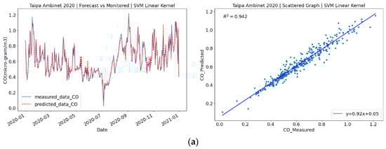
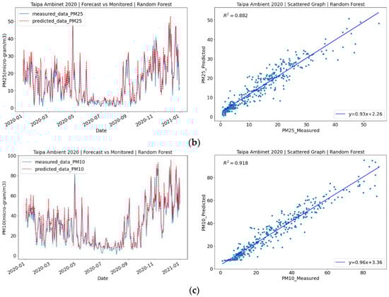
Figure 2.
(a) Measured and predicted CO concentrations using SVM; (b) PM2.5 and (c) PM10 predictions using RF for 2020.
Figure 3 shows the SHAP values of the variables for the SVM model for CO prediction and the RF model for PM2.5 and PM10 prediction in 2020. It indicates that the CO concentration of 16D1 is a significant feature that influences the prediction result, and its importance is 0.55. There is a positive relationship between the CO concentration of 16D1 and the predicted CO concentration. In addition, the T_AIR_MX (ground level max temperature), the WDIR (wind direction); the TD_850 and the H_850 (the dew point and geopotential at 850hPa in upper air) are other features which contribute to the forecast model. The dominant feature is PM25_16D1, with its importance being 11.18 in the PM2.5 model. The second most important feature is PM25_23D1. There is a positive relationship between the model output and PM25_16D1. The other features which contributed to the forecast model were DD, STB_925, VMED, WDIR, H_850, and H_700. Also, PM10_16D1 contributed the most to the PM10 model output. The other features which contributed to the PM10 forecast model are DD, HRMN, HRMD, TD_MD, VMED, and TAR_850.
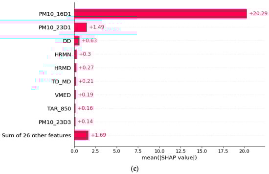
Figure 3.
(a) SHAP values of each variable in the SVM model for CO prediction; RF model for (b) PM2.5 and (c) PM10 prediction in 2020.
To confirm the significance of meteorological features on the predictive ability of the 24-h ML models, the adjusted R2 values were calculated for the models, with and without, meteorological features. Table 4 shows the R2 and adjusted R2 values in 2020. The reliability of the 24-h forecast model can be confirmed by the adjusted R2 value of the feature combination (all variables included) which is higher than the model with only pollutant concentration. The adjusted R2 value of the model with upper air observation and surface observation can be used as an indicator to determine feature reduction.
Table 4.
Comparison of Adjusted R2 for all best ML models (24-h) in 2020.
3.2. Performance of ML Models in 2021 (24 h)
The performance of the ML models, including ANN, RF, XGBoost, SVM, and MLR, was determined by a comparison of the R2 value. Table 5 shows the detailed performance of each ML model in 2021. The best results are highlighted in bold. The best-performing model for PM2.5 was the RF model with an R2 of 0.89, for PM10 it was the SVM model with an R2 of 0.92, and for CO it was the ANN model with an R2 of 0.79. The performance of the RF, SVM and ANN models is better than that of the MLR model. The ANN model showed good performance in 2021 in comparison to the previous year in 2020. The SVM model showed a significant drop in the forecast performance for CO in 2021 (R2 of 0.76) compared to the prediction in 2020 (R2 of 0.94). The variable “DD” was found to be insignificant on the R2 in 2021. The best model for CO prediction is the ANN model, with an R2 of 0.77 and an adjusted R2 of 0.75 after “DD” is reduced. The adjusted R2 value without DD reduction was 0.76.
Table 5.
Overview of the RF, ANN, XGBoost, and SVM models trained with the 2017–2020 dataset and validated with the 2021 dataset.
Air quality prediction for the 2021 dataset did not require feature selection, but it was required for CO in 2020. Although CO has the lowest R2 value compared to PM10 and PM2.5, the RMSE, MAE, and BIAS values are low and reasonable. The drop in R2 value could be caused by the sudden change in the emission trend from 2019 to 2021. CO emissions increased in 2021 during the new normal period of the COVID-19 pandemic, but the levels of PM2.5 and PM10 concentrations remained unaffected.
Figure 4 shows the prediction result of CO using the ANN model, and PM2.5 and PM10 using the RF model for 2021. It shows that the prediction value is lower than the observation value with an R2 of 0.79, and there are a few outliers. The sudden change in CO emissions is primarily due to the COVID-19 pandemic in 2020 and has slowly increased by 3% in the new normal period in 2021. The predicted result of the RF model fits well with the observation value of PM2.5. The R2 is 0.89. Most values of PM2.5 could be predicted accurately. However, the extreme high and low pollution episodes are difficult to capture using the RF model. It also shows the prediction results of the SVM model for PM10 in 2021. The SVM linear kernel works well in this task. The R2 is 0.92, with the prediction value slightly lower than the observation value.
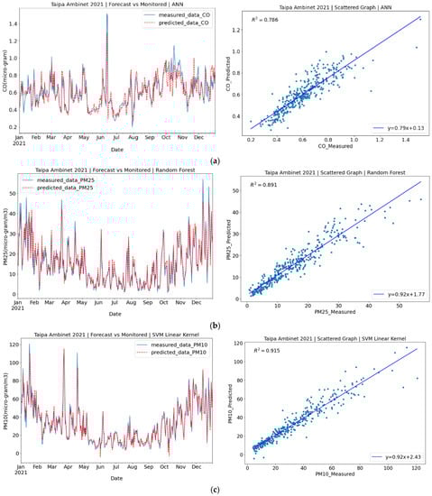
Figure 4.
(a) Measured and predicted CO concentrations using the ANN model; Measured and predicted (b) PM2.5 and (c) PM10 concentrations using the RF model for 2021.
Figure 5 shows the SHAP values of each variable in different models, with CO_16D1 being the most important feature and T_AIR_MX being the second most important feature that contributes to the prediction results. The other features with contributions to the model are TD_850, H_850, WDIR, T_AIR_MN, DD, T_AIR_MD, and STB_700. It shows that PM25_16D1 is the most important feature, while PM25_23D1 is the second most important feature that contributes to the prediction results. The other features with contributions to the model are STB_925, STB_700, H_850, TAR_850, VMED, and TD_MD. Also, it shows that PM10_16D1 is the most important feature, while PM10_23D1 and THI850 also show a significant contribution to the model.
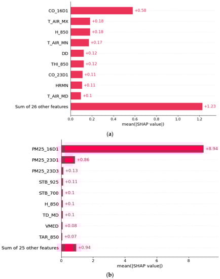
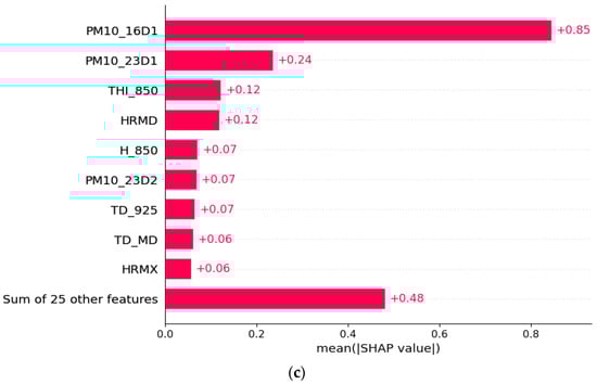
Figure 5.
(a) SHAP values of each variable for the ANN model in 2021 CO prediction; (b) RF model in 2021 PM2.5 prediction; (c) SVM model in 2021 PM10 prediction.
To confirm the significance of meteorological features on the predictive ability of the 24-h ML models, the adjusted R2 values were calculated for the models, with and without, meteorological features. Table 6 shows the R2 and adjusted R2 values for 2021. The reliability of the 24-h forecast model can be confirmed by the adjusted R2 value of the feature combination (all variables included) which is higher than the model with only pollutant concentration. The adjusted R2 value of the model with upper air observation and surface observation can be used as an indicator to determine feature reduction.
Table 6.
Comparison of Adjusted R2 for all best ML model (24-h) in 2021.
3.3. Performance of ML Models (48-h)
The performance of the ML models, including ANN, RF, XGBoost, SVM, and MLR, is determined by a comparison of the R2 values. Table 7 shows the detailed performance of each ML model separately. The best results are highlighted in bold. The RF model was found to have the best performance in PM10 with an R2 of 0.66, the SVM model showed the best prediction in PM2.5 with an R2 of 0.55, and the CO with an R2 of 0.62. The performance of 48-h forecasting for PM10, PM2.5, and CO shows a deterioration with a moderate R2 value (from 0.55 to 0.66) in comparison to the 24-h forecast.
Table 7.
Comparison of the RF, ANN, XGBoost, SVM and MLR models trained by 2016–2019 data and tested on 2020 data. (48-h forecast).
The 48-h model needs an assessment of the meteorological factors which significantly influence it with the adjusted R2 test. Table 8 shows the meteorological features that influence the accuracy of the 48-h ML models by comparing the adjusted R2 values in combination, with and without, meteorological features with the adjusted R2 value without feature selection.
Table 8.
Comparison of Adjusted R2 for all the best ML models (48-h) in 2020.
The SVM model shows the best performance in the 48-h forecast model for the prediction of CO. Figure 6 shows the measured and predicted CO using the SVM model, and PM2.5, and PM10 using the RF model in 2020. It shows that the prediction value is often lower than the observation value in high pollution episodes during the winter season, with an R2 value of 0.62. The SVM model obtained an R2 value of 0.57 for PM2.5 prediction. The performance of the SVM model was better than the other ML models. It shows that the SVM model predicted very poorly in the high pollution episodes, with an R2 of 0.55. The SVM model could not predict well the high and low pollution episodes. The RF model showed the best performance in the forecasting of PM10, with an R2 value of 0.66. It also shows that the RF model was unable to predict extremely high and low pollution episodes.
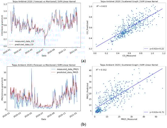
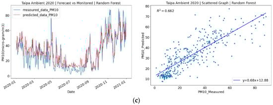
Figure 6.
(a) Measured and predicted CO (48-h) concentrations using SVM for 2020; (b) PM2.5 (48 h) concentrations using SVM for 2020; (c) PM10 (48 h) concentrations using RF for 2020.
3.4. Limitation of the Study
Some of the limitations of the study were records with blank data being found over two months (from August to October 2017) due to the AQMS malfunction caused by a super typhoon. The blank data records may negatively impact the accuracy of the ML models. Despite the good performance of the ML models, it may be difficult to capture some of the very low or high pollution episodes in a special scenario, such as the outbreak of the COVID-19 pandemic in early 2020. The result of this study is very similar to studies in other regions [34,35], with a high R2 and low RMSE and MAE.
4. Conclusions
The application of different ML methods to predict the next day 24-h concentration of CO, PM2.5, and PM10 from 2020 to 2021, and build a reduced-feature forecast model for the 48 h forecast in the concentration CO, PM2.5 and PM10, were successful for Taipa Ambient AQMS in the region of Macau. The results of the 24-h model demonstrated that it was more difficult to predict the CO concentration in 2021 with the lowest R2 compared to the PM10 and PM2.5 results. The 48-h forecast model was found to be challenging for PM2.5, with an R2 value of 0.55. In all the ML models, the variable of pollutant concentration (CO, PM2.5, and PM10) in 16D1, D2, and D3 played an essential role in predicting CO, PM2.5, and PM10 with the other meteorological features in the upper air and surface ground level. For the 48-h model, it is required to build a reduced-feature model based on 24-h features. Eventually, the feature selection was conducted successfully based on the SHAP value summary and other selection criteria. The meteorological features were selected systematically and confirmed by adjusting R2 to ensure the highest R2 value was achieved. The meteorological features were critical in increasing the accuracy of predicting pollutant concentration. In conclusion, all of the ML algorithms were able to successfully forecast the 24 and 48 h of pollutant concentration in Macau, with RF and SVM performing the best in the prediction of PM2.5 and PM10, and CO in both 24 and 48-h forecasts. Nevertheless, using more years of datasets from neighboring regions may be considered for improving forecasting ability in future studies.
Author Contributions
Conceptualization, T.M.T.L. and S.C.W.N.; methodology, T.M.T.L. and S.W.I.S.; software, T.M.T.L., S.C.W.N. and S.W.I.S.; validation, T.M.T.L. and S.W.I.S.; data curation, T.M.T.L. and S.C.W.N.; writing—original draft preparation, T.M.T.L. and S.C.W.N.; writing—review and editing, T.M.T.L. and S.W.I.S.; supervision, T.M.T.L. and S.W.I.S.; funding acquisition, T.M.T.L. All authors have read and agreed to the published version of the manuscript.
Funding
This research received no external funding.
Data Availability Statement
3rd Party Data. Restrictions apply to the availability of these data.
Acknowledgments
The work developed was supported by The Macao Meteorological and Geophysical Bureau (SMG).
Conflicts of Interest
The authors declare no conflict of interest.
References
- Mendes, L.; Monjardino, J.; Ferreira, F. Air Quality Forecast by Statistical Methods: Application to Portugal and Macao. Front. Big Data 2022, 5, 826517. [Google Scholar] [CrossRef] [PubMed]
- Lei, T.M.; Siu, S.W.; Monjardino, J.; Mendes, L.; Ferreira, F. Using Machine Learning Methods to Forecast Air Quality: A Case Study in Macao. Atmosphere 2022, 13, 1412. [Google Scholar] [CrossRef]
- Li, X.; Lopes, D.; Mok, K.M.; Miranda, A.I.; Yuen, K.V.; Hoi, K.I. Development of a road traffic emission inventory with high spatial–temporal resolution in the world’s most densely populated region—Macau. Environ. Monit. Assess. 2019, 191, 239. [Google Scholar] [CrossRef]
- Azarov, V.; Manzhilevskaya, S.; Petrenko, L. The Pollution Prevention during the Civil Construction. EDP Sci. 2018, 196, 04073. [Google Scholar] [CrossRef]
- Lee, Y.C.; Savtchenko, A. Relationship between Air Pollution in Hong Kong and in the Pearl River Delta Region of South China in 2003 and 2004: An Analysis. J. Appl. Meteorol. Climatol. 2006, 45, 269–282. [Google Scholar] [CrossRef]
- Fang, X.; Fan, Q.; Li, H.; Liao, Z.; Xie, J.; Fan, S. Multi-scale correlations between air quality and meteorology in the Guangdong−Hong Kong−Macau Greater Bay Area of China during 2015. Atmos. Environ. 2018, 191, 463–477. [Google Scholar] [CrossRef]
- Tong, C.H.M.; Yim, S.H.L.; Rothenberg, D.; Wang, C.; Lin, C.Y.; Chen, Y.D.; Lau, N.C. Projecting the impacts of atmospheric conditions under climate change on air quality over the Pearl River Delta region. Atmos. Environ. 2018, 193, 79–87. [Google Scholar] [CrossRef]
- Bernstein, J.A.; Alexis, N.; Barnes, C.; Bernstein, I.L.; Bernstein, J.A.; Nel, A.; Peden, D.; Diaz-Sanchez, D.; Tarlo, S.M.; Williams, P.B. Health effects of air pollution. J. Allergy Clin. Immunol. 2004, 114, 1116–1123. [Google Scholar] [CrossRef] [PubMed]
- Fang, X.; Fan, Q.; Liao, Z.; Xie, J.; Xu, X.; Fan, S. Spatial-temporal characteristics of the air quality in the Guangdong−Hong Kong−Macau Greater Bay Area of China during 2015. Atmos. Environ. 2019, 210, 14–34. [Google Scholar] [CrossRef]
- Sheng, N.; Tang, U.W. Risk assessment of traffic-related air pollution in a world heritage city. Int. J. Environ. Sci. Technol. 2013, 10, 11–18. [Google Scholar] [CrossRef]
- Valavanidis, A.; Fiotakis, K.; Vlachogianni, T. Airborne Particulate Matter and Human Health: Toxicological Assessment and Importance of Size and Composition of Particles for Oxidative Damage and Carcinogenic Mechanisms. J. Environ. Sci. Health Part C 2008, 26, 339–362. [Google Scholar] [CrossRef] [PubMed]
- Londahl, J.; Massling, A.; Pagels, J.; Swietlicki, E.; Vaclavik, E.; Loft, S. Size-Resolved Respiratory-Tract Deposition of Fine and Ultrafine Hydrophobic and Hygroscopic Aerosol Particles During Rest and Exercise. Inhal. Toxicol. 2010, 19, 109–116. [Google Scholar] [CrossRef] [PubMed]
- Lin, Y.; Zou, J.; Yang, W.; Li, C.Q. A Review of Recent Advances in Research on PM2.5 in China. Int. J. Environ. Res. Public Health 2018, 15, 438. [Google Scholar] [CrossRef] [PubMed]
- Wittenberg, B.A.; Wittenberg, J.B. Effects of carbon monoxide on isolated heart muscle cells. Res. Rep. Health Eff. Inst. 1993, 62, 1–21. [Google Scholar]
- Townsend, C.L.; Maynard, R.L. Effects on health of prolonged exposure to low concentrations of carbon monoxide. Occup. Environ. Med. 2002, 59, 708–711. [Google Scholar] [CrossRef] [PubMed]
- Shimadera, H.; Kojima, T.; Kondo, A. Evaluation of Air Quality Model Performance for Simulating Long-Range Transport and Local Pollution of PM2.5 in Japan. Adv. Meteorol. 2016, 2016, 5694251. [Google Scholar] [CrossRef]
- Kahraman, A.C.; Sivri, N. Comparison of metropolitan cities for mortality rates attributed to ambient air pollution using the AirQ model. Environ. Sci. Pollut. Res. 2022, 29, 43034–43047. [Google Scholar] [CrossRef] [PubMed]
- Xue, W.; Wang, Y. Domestic and Foreign Research Progress of Air Quality. Environ. Sustain. Dev. 2013, 38, 14–20. [Google Scholar]
- Chaloulakou, A.; Kassomenos, P.; Spyrellis, N.; Demokritou, P.; Koutrakis, P. Measurements of PM10 and PM2.5 particle concentrations in Athens, Greece. Atmos. Environ. 2003, 37, 649–660. [Google Scholar] [CrossRef]
- Elangasinghe, M.A.; Singhal, N.; Dirks, K.N.; Salmond, J.A. Development of an ANN–based air pollution forecasting system with explicit knowledge through sensitivity analysis. Atmos. Pollut. Res. 2014, 5, 696–708. [Google Scholar] [CrossRef]
- Maleki, H.; Sorooshian, A.; Goudarzi, G. Air pollution prediction by using an artificial neural network model. Clean Technol. Environ. Policy 2019, 21, 1341–1352. [Google Scholar] [CrossRef]
- Sinnott, R.O.; Guan, Z. Prediction of Air Pollution through Machine Learning Approaches on the Cloud. In Proceedings of the 2018 IEEE/ACM 5th International Conference on Big Data Computing Applications and Technologies (BDCAT), Zurich, Switzerland, 17–20 December 2018. [Google Scholar]
- Suárez Sánchez, A.; Garcia Nieto, P.J.; Riesgo Fernández, P.; del Coz Díaz, J.J.; Iglesias-Rodriguez, F.J. Application of an SVM-based regression model to the air quality study at local scale in the Avilés urban area (Spain). Math. Comput. Model. 2011, 54, 1453–1466. [Google Scholar] [CrossRef]
- Bhattacharya, E.; Bhattacharya, D. A Review of Recent Deep Learning Models in COVID-19 Diagnosis. Eur. J. Eng. Technol. Res. 2021, 6, 10–15. [Google Scholar] [CrossRef]
- Yu, R.; Yang, Y.; Yang, L.; Han, G.; Move, O.A. RAQ-A Random Forest Approach for Predicting Air Quality in Urban Sensing Systems. Sensors 2016, 16, 86. [Google Scholar] [CrossRef] [PubMed]
- Liu, H.; Lang, B. Machine Learning and Deep Learning Methods for Intrusion Detection Systems: A Survey. Appl. Sci. 2019, 9, 4396. [Google Scholar] [CrossRef]
- Pan, B. Application of XGBoost algorithm in hourly PM2.5 concentration prediction. In IOP Conference Series Earth and Environmental Science; IOP Publishing: Bristol, UK, 2018; p. 113. [Google Scholar]
- Jiao, W.; Frey, H.C. Comparison of Fine Particulate Matter and Carbon Monoxide Exposure Concentrations for Selected Transportation Modes. Transportation Research Record. J. Transp. Res. Board 2014, 2428, 54–62. [Google Scholar] [CrossRef]
- Awad, M.; Khanna, R. Support Vector Regression. In Efficient Learning Machines; Springer: Cham, Switzerland, 2015; pp. 67–80. [Google Scholar]
- Breiman, L. Random Forests. Mach. Learn. 2001, 45, 5–32. [Google Scholar] [CrossRef]
- Chen, T.; Guestrin, C. XGBoost: A Scalable Tree Boosting System. In Proceedings of the 22nd ACM SIGKDD International Conference on Knowledge Discovery and Data Mining (KDD ‘16); Association for Computing Machinery: New York, NY, USA, 2016; pp. 785–794. [Google Scholar]
- Lundberg, S.M.; Lee, S.I. A Unified Approach to Interpreting Model Predictions. Adv. Neural Inf. Process. Syst. 2017, 30, 4766–4775. [Google Scholar]
- Rozemberczki, B.; Watson, L.; Bayer, P.; Yang, H.T.; Kiss, O.; Nilsson, S.; Sarkar, R. The Shapley Value in Machine Learning. arXiv 2022, arXiv:2202.05594. [Google Scholar]
- Akbal, Y.; Ünlü, K.D. A deep learning approach to model daily particular matter of Ankara: Key features and forecasting. Int. J. Environ. Sci. Technol. 2021, 19, 5911–5927. [Google Scholar] [CrossRef]
- Esager, M.W.M.; Ünlü, K.D. Forecasting Air Quality in Tripoli: An Evaluation of Deep Learning Models for Hourly PM2.5 Surface Mass Concentrations. Atmosphere 2023, 14, 478. [Google Scholar] [CrossRef]


Disclaimer/Publisher’s Note: The statements, opinions and data contained in all publications are solely those of the individual author(s) and contributor(s) and not of MDPI and/or the editor(s). MDPI and/or the editor(s) disclaim responsibility for any injury to people or property resulting from any ideas, methods, instructions or products referred to in the content. |
© 2023 by the authors. Licensee MDPI, Basel, Switzerland. This article is an open access article distributed under the terms and conditions of the Creative Commons Attribution (CC BY) license (https://creativecommons.org/licenses/by/4.0/).