Abstract
The direct application of the Hoek–Brown failure criterion to practical slope engineering is still an urgent problem. The slope geometries and earthquake effect need to be considered in the determination of linear Mohr–Coulomb (MC) strength parameters from the Hoek–Brown criteria for slope stability analysis. This study adopted the tangential method to construct a three-dimensional (3D) rotational failure mechanism using the Hoek–Brown failure criterion for homogeneous rock slopes undergoing earthquake. The quasi-static method was employed to treat the seismic action as an external seismic force in the work–energy equation of the limit analysis theory. Based on the numerical optimization, the least upper-bound solutions and equivalent MC strength parameters were derived with respect to different strength parameters and seismic loads. The influences of nonlinear strengths, geometric parameters and earthquake load on the equivalent MC strength parameters were thoroughly investigated. The results suggested that the nonlinear parameters have different influences on the equivalent MC parameters for general steep slopes and vertical slopes. The effects of nonlinear parameters on the equivalent MC parameters become obvious for vertical slopes. The disturbance factor D affects the equivalent MC parameters only for very steep slopes in fractured rock masses. Additionally, the effect of slope inclination on the equivalent MC parameters becomes obvious for slopes in fractured hard rock masses. The 3D effect of the rock slope on the equivalent MC parameters was found to be slight. Moreover, the impact of earthquakes on the approximate MC parameters becomes weaker for steeper rock slopes. The tables of approximate MC strength parameters were given for various slopes with different nonlinear strength parameters. The presented tables can provide certain references for practical slope engineering.
1. Introduction
Landslides are a common geological disaster. Slope stability problems have gained extensive attention from scholars in mining engineering and geotechnical engineering fields, both domestically and abroad. For slopes in soils and rocks, the Mohr–Coulomb (MC) strength envelope, represented by the friction angle and the cohesion, has been widely used in conventional slope analysis methods, computer software, and engineering standards for slope design. Based on experimental data, the nonlinearity of geomaterial shear strengths has been illustrated by many studies [1,2,3,4,5]. Hoek and Brown [2] proposed the early experience expression of the nonlinear Hoek–Brown (HB) failure criterion to evaluate the shear strengths of intact rock or rock masses. Since then, Hoek et al. and other studies [6,7,8,9,10,11] have further developed and improved this HB failure criterion. Currently, the HB criterion is widely accepted, and many attempts have been made to solve various rock slope stability problems [12,13,14,15,16].
Since the HB strength criterion is not expressed by two MC strength parameters, direct application to the slope engineering standards and strength reduction methods for slope stability analysis presents difficulties. To meet the requirements of slope engineering in practice, Hoek and his team [2,6,7,8,9] committed to determine the analytical formulas of the average MC parameters from the HB criterion of strength parameters. But the obtained average MC strength parameters are specific to the minimum principal stress range. The analytical formulas were later developed by other studies to estimate the MC parameters for rocks governed by the HB strength criterion [17,18,19,20,21]. Yang and Yin [22] derived the equivalent MC parameters from the HB criterion for the ultimate bearing capacity of a rock foundation by using the limit analysis method. Shen et al. [23] proposed an approximate analytical method to estimate the MC strength parameters for two-dimensional (2D) slope stability analysis. Ren et al. [24] used the numerical method to calculate the instantaneous equivalent MC parameters, based on of the stress distribution along the slope slip surface. These studies illustrated that a more accurate estimation of the equivalent MC parameters from the HB criterion can be made by considering the slope problem and its analysis method. Studies should be carried out to delve into the influences of slope geometries (i.e., slope inclination and 3D effect) and nonlinear strength parameters on the determination of equivalent MC strengths for slopes.
Earthquakes are one of the main factors inducing landslide accidents. For the safety of 2D and 3D slopes satisfying the HB yield criterion, some studies have been performed to assess the seismic stability and seismic displacement of rock slopes by using the limit analysis method [11,13,25,26,27] and numerical methods [14,28]. These have revealed that the slope’s safety will decrease, and the location of the slope slip surface will change as the seismic action becomes stronger. These findings illustrated that the stress range along the slope slip surface varies for slopes undergoing different earthquakes. The earthquake may have a potential influence on the equivalent MC parameters, which needs to be further investigated.
Considering these existing problems, the determination method for equivalent MC parameters from the HB criterion should be established for 3D slopes undergoing earthquakes. Further studies should be performed to investigate the effects of seismic action, geometric parameters and nonlinear strengths on the equivalent MC parameters. Hence, this paper used the quasi-static method to conduct the 3D limit analysis approach for the determination of equivalent MC parameter for seismic stability analysis of slopes obeying the HB criterion. The approximate MC strength parameters can be determined when the least upper-bound solutions for slope stability are derived. Subsequently, the effects of the HB parameters on the equivalent MC strength parameters are analyzed for slopes with different slope geometries (slope inclination and 3D effect) and seismic loads. These analyses can also illustrate how slope geometries and earthquakes affect the equivalent MC strength parameters. In addition, charts of approximate MC parameters are provided as certain references for slope engineering.
2. Estimating MC Parameters from the HB Criterion for 3D Slopes
2.1. The HB Strength Criterion
For intact rock and rock masses, Hoek at al. [9] presented a generalized expression of the HB failure criterion, which can be expressed as the following Equation (1):
where the parameters σ1 and σ3 relate to the total major and minor principal stresses, respectively. The parameter σci is the uniaxial compressive strength of the intact rock, which is generally in the range of 0.25–250 MPa [8]. The parameters mb, s and α are defined as these following expressions of Equations (2)–(4):
in which, the parameter mi is the rock material constant and its referential values for five kinds of rocks can be found in the study of Hoek [6]. The parameter GSI is the geological strength index, which has a range of 0 to 100. As the value of GSI increases, the rock mass will be more complete with a smaller degree of fragmentation. The parameter D represents the disturbance coefficient, which ranges from 0 to 1. As illustrated by Hoek et al. [9], the generalized HB failure criterion is more suitable for the intact rock and severely broken rock mass. Since the presented limit analysis method in this paper is commonly applied for homogeneous slope problems, the generalized HB criterion can be easily utilized in the establishment of the following limit analysis approach.
2.2. Tangent Technique
As shown in Equation (1), the strength criterion cannot be converted into the expression in forms of the friction angle ϕ and the cohesion c. These two strength parameters will change at different normal stress σn. This will cause difficulty in applying the nonlinear HB criterion in the stability evaluation of rock slopes. The tangential technique was proposed and developed to address this difficulty in the limit analysis of slope stability [13,25,26,29,30]. As illustrated in Figure 1, the nonlinear HB strength envelope can be simplified by an instantaneous linear criterion in a certain stress range. The corresponding equivalent MC strength parameters of the tangent line can approximately reflect the average shear strengths in the stress range along the slope’s sliding surface. The adequacy and accuracy of upper bound solutions derived from the tangential technique have been well studied and verified by some studies [14,31]. The instantaneous tangent line at a point G can be expressed as the following Equation (5):
where τ and σn denote the shear stress and normal stress along the slope slip surface, respectively. Parameter ϕe is the instantaneous inclination of the tangent line, which is called the equivalent friction angle in this study. Parameter ce is the instantaneous intercept of the tangent line at the τ axis, which is defined as the equivalent cohesion.
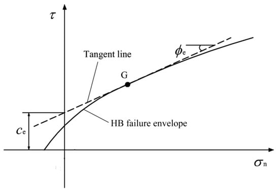
Figure 1.
The HB failure envelope and tangent line.
Using the Equations (6) and (7) for σn and τ (in forms of total major principal stress σ1 and total minor principal stress σ3) in the Mohr stress circle:
and
The expression of the HB strength criterion (Equation (1)) can be transformed into the formula of σn with respect to τ, as shown in Equation (8):
Making dσn/dτ = 1/ tanϕe in Equation (8), the parameter τ can be derived as a function of ϕe, that is shown in Equation (9):
Substituting Equation (9) into Equation (8), the expression of σn in the form of ϕe will be obtained from the following Equation (10):
Finally, substituting Equations (9) and (10) into the tangent line Equation (8), the equivalent cohesion ce can be given as a function of ϕe, which has the following Equation (11):
To simply the use of the above Equation (11) in the subsequent limit analysis approach, the dimensionless ratio ce/σci will be used as the equivalent cohesion. The practicable equivalent cohesion ce will be calculated by multiplying the uniaxial compressive strength of the intact rock σci.
2.3. Limit Analysis for 3D Slopes
The limit analysis method is based on a kinematically admissible velocity field, which satisfies the velocity boundary condition and the orthogonal flow rule. For a kinematically admissible velocity field, an upper bound on the limit load and the corresponding critical slip surface are determined by the energy rate balance equation. The kinematically admissible velocity field defines the possible mechanism of failure, which is generally called the “rotational failure mechanism”.
For homogeneous isotropic soil slopes governed by the linear MC failure criterion, Michalowski and Drescher [32] presented the 3D toe-failure mechanism for limit analysis of slope stability. This 3D failure mechanism was then widely applied, and further developed in the limit analysis approach of slope stability [33,34,35,36]. As is known, the inclination of actual rock slopes is generally large. For homogeneous isotropic rock slopes, this 3D toe-failure mechanism can be used to solve rock slope problems. For instance, Gao et al. [15] and Xu et al. [34] combined the nonlinear HB envelope into the 3D failure mechanism to conduct the limit analysis for the stability of slopes in homogeneous rock masses. These studies suggest that the 3D failure mechanism can provide an accurate estimate of the upper bound on the stability of 3D slopes. Hence, this paper utilized the 3D failure mechanism with the HB criterion to establish the limit analysis method for rock slopes undergoing earthquakes.
As presented in Figure 2, the 3D failure mechanism with the HB failure envelope has the slip surface through the slope toe, which can be called the toe-failure mechanism. The 3D failure mechanism is composed of two parts: a curvilinear cone and a plane insertosome. The slope height is H, and the slope inclination is β. The total slope width is marked by B. The width of the plane insertosome is marked by b. The 3D mechanism can degrade into the plane strain 2D mechanism once the relative width B/H reaches infinity. Additionally, the apex angle of failure mechanism is presented by an added variable ϕe, which also determines the tangent point location for the HB criterion. The specific definitions for the variables in Figure 2, and the comprehensive descriptions of this failure mechanism, can be found in the references [15,33].
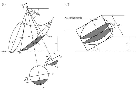
Figure 2.
3D failure mechanism: (a) side view; (b) oblique view [33].
In view of the earthquake effect, the quasi-static method has been widely applied in slope stability assessment [13,14,26]. The seismic action is represented by a horizontal and vertical acceleration, which is uniformly distributed throughout the whole sliding body. Since vertical acceleration can be reflected in the increase in gravitational acceleration, the results for analyzing the dynamic stability of slopes by using vertical acceleration will have a linear proportional relationship with those for the static stability of slopes. Hence, vertical acceleration was ignored in this study. The seismic load can be calculated by multiplying the soil self-weight with the horizontal seismic acceleration coefficient kh. The range of the seismic acceleration coefficient kh is always between 0.0 and 0.3.
In this 3D failure mechanism, the slip body is under the forces of self-weight stress and horizontal seismic stress. According to the limit analysis theory, the work–energy function is established by making two external work rates (self-weight work rate Wγ and horizontal seismic work rate Ws) equal to the internal energy dissipation rate D. Hence, the work–energy equation can be written as the following Equation (12):
in which, the superscripts “curve” and “plane” are used to distinguish the energy rates for the curvilinear cone and plane insertosome, respectively. For self-weight work rate and internal energy dissipation rate Dcurve of the curvilinear cone part, see specific expressions in the references of Gao et al. [15]. The expressions for and Dplane of the insertosome part can be found in the study of Yang et al. [13]. The horizontal seismic work rate Ws also consists of for curvilinear cone and for plane insertosome. The expressions for and can be calculated by the below Equations (13) and (14) [37]:
where the variables a, d and θB, and the functions of fs1, fs2, and fs3, can be derived as in the following expressions of Equations (15)–(23) [37]:
where ω relates to the angular velocity, γ is the soil unit weight, and β represents the slope inclination. As shown in Figure 2, r0 and r0′ represent the distances OA and OA′. The other parameters a, d1, θ0, θB, θh, R, and rm have been marked in this figure. Similar expressions for , and related Equations (15)–(23) have been presented in the study of Michalowski and Martel [37]. However, it is noted that the friction angle ϕ in their equations should be replaced by the equivalent friction angle ϕe.
Based on the energy–balance equation (Equation (12)), an upper bound on the slope stability number N = γH/σci (γ is unit weight of rock mass and H is slope height) will be calculated when the slope failure mechanism is chosen for a given slope with the seismic load. Here, the safety factor (FOS) for rock slopes is equal to 1.0. The stability number γH/σci is defined as a dimensionless critical height in limit state, which can be used for the preliminary assessment on the critical height Hcr of slopes in design or excavation.
To derive the least upper bound on slope stability number, an optimization procedure written in a MATLAB software code will be performed by changing the geometry and location of failure mechanism in regard to five variables: θ0, θh, ϕe, r0′/r0, and b/B. Here, the notation b represents the width of plane insertosome and B represents the total slope width. The definitions of variables θ0 and θh can be seen in Figure 2. Once the critical value of slope stability N is obtained, the critical slip failure and the tangent line location of the HB criterion will also be determined by the optimized variables θ0, θh, ϕe, r0′/r0, and b/B.
2.4. Estimating MC Strength Parameters
As presented in the above section, the equivalent friction angle ϕe plays an important role in the 3D limit analysis method with the nonlinear HB criterion. The equivalent friction angle ϕe determines the location of the tangent point on the HB strength envelope. Additionally, it is also a variable denoting the apex angle of the 3D failure mechanism. When the least upper-bound solution for a given slope is derived in the optimization procedure, the value of the variable ϕe will be obtained. Meanwhile, the equivalent cohesion ce will be calculated from the function of Equation (11). In this situation, the normal stress distribution along the slope slip surface will be in a specific range. The obtained tangent line may best represent the upper bound on the shear strengths of the HB strength envelope in this normal stress scope. Hence, the calculated parameters ϕe and ce can be utilized as approximate values of MC strength parameters to solve slope stability problems.
3. Results and Discussions
3.1. Effect of the HB Parameters on Equivalent MC Strengths
Two 3D static slopes with β = 45° and 90° were selected as examples. Figure 3 and Figure 4 show the curves of equivalent internal friction angle ϕe and equivalent cohesion ce/σci varying with the rock material constant mi, respectively. The slope width to slope height (i.e., the ratio B/H) is adopted as 2.0, and value of the disturbance coefficient D is 0. In each diagram, three curves were drawn under the conditions that the geological strength index GSI is 10, 50 and 100. By comparing Figure 3 and Figure 4, it can be seen that the influences of rock material constant mi on equivalent MC parameters are quite different under slopes with different inclinations. As shown in Figure 3, the equivalent internal friction angle ϕe for a slope with β = 45° increases slightly and eventually tends to be constant with the increase in the rock material constant mi. The equivalent cohesion ce/σci also shows an increasing trend with the increase in mi. The influence of mi on equivalent MC parameters will be more remarkable as the GSI value becomes bigger. It is known that the fragmentation degree of rock masses will decrease with an increasing GSI value. For slopes in rock masses with fewer fractures, the slope’s stability and its equivalent strength parameters tend to be more sensitive to the rock material, which is estimated by the parameter mi. However, for vertical slopes in Figure 4, the equivalent internal friction angle ϕe gradually increases and the equivalent cohesion ce/σci tends to decrease as mi. increases. The degree of influence of mi on the equivalent MC parameters is almost entirely unaffected by the GSI value. Since the slip surface of a vertical slope is shallow and its slide mass is small, the fragmentation degree of rock masses tends to have only slight influence on the changing laws of the equivalent strength parameters, with respect to the parameter mi.
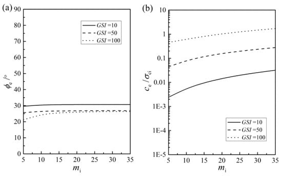
Figure 3.
Influence of mi on equivalent MC parameters (β = 45°): (a) equivalent internal friction angle ϕe; (b) equivalent cohesion ce/σci.
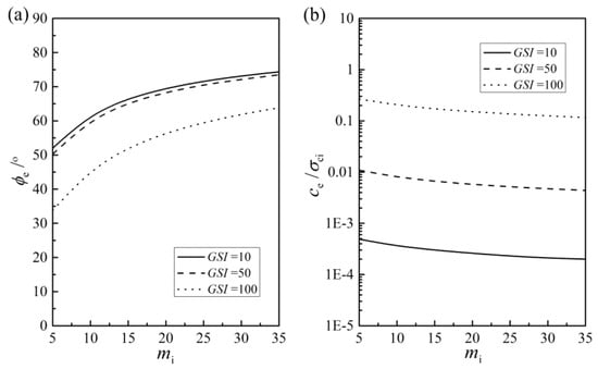
Figure 4.
Influence of mi on equivalent MC parameters (β = 90°): (a) equivalent internal friction angle ϕe; (b) equivalent cohesion ce/σci.
Figure 5 and Figure 6 illustrated the influence of the GSI on the equivalent strength parameters ϕe and ce/σci. Similarly, the width-to-height ratio B/H for two static slopes is 2.0 and the disturbance factor D is 0. To take account of the effect of the material constant mi, two cases of mi = 10 and mi = 25 were given in each figure. Figure 5 and Figure 6 reveal that the GSI has a slightly different influence on the equivalent MC parameters for different slopes. As shown in Figure 5, the equivalent internal friction angle ϕe for slopes with β = 45° decreases slightly with an increasing GSI, but the equivalent cohesion ce/σci increases significantly. The degree of influence of the GSI value on the equivalent MC parameters appears to be evident as mi decreases. Nevertheless, for vertical slopes (β = 90°), Figure 6 shows that the equivalent internal friction angle ϕe tends to increase slightly and then decrease with the increasing GSI. The equivalent cohesion ce/σci grows larger with the increasing GSI. The effect of the GSI on equivalent MC parameters does not vary significantly when considering different values of mi.
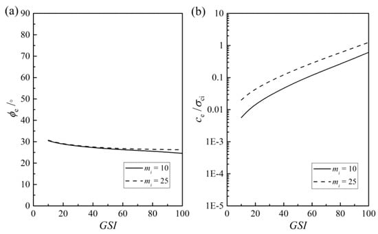
Figure 5.
Influence of GSI on equivalent MC parameters (β = 45°): (a) equivalent internal friction angle ϕe; (b) equivalent cohesion ce/σci.
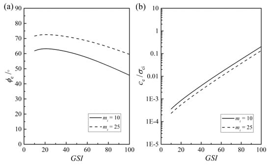
Figure 6.
Influence of GSI on equivalent MC parameters (β = 90°): (a) Equivalent internal friction angle ϕe; (b) Equivalent cohesion ce/σci.
As shown in Figure 7 and Figure 8, the variation curves of the equivalent parameters ϕe and ce/σci with respect to different disturbance factors D were given for two static slopes with β = 45° and β = 90°. Here, the rock material constant mi was taken as 20, and the slope relative width B/H was taken as 2.0. Different values of the geological strength index GSI were considered in three cases: GSI = 10, GSI = 50 and GSI = 90. For two slopes in Figure 7 and Figure 8, the disturbance factor D has different effects on the equivalent MC parameters. For slopes with β = 45° (Figure 7), the effect of D on the equivalent internal friction angle ϕe is slight, but the equivalent cohesion ce/σci decreases with the increasing D value. This decreasing trend becomes less pronounced as the GSI increases. Especially when the GSI is 90, the curve of ce/σci becomes a near-horizontal line with a varying D value. For vertical slopes in Figure 8, the equivalent internal friction angle ϕe and the equivalent cohesive force ce/σci both tend to decrease as D increases, and this decreasing trend also becomes slight with the increase in the GSI. Similarly, D hardly affects the equivalent internal friction angle ϕe and the equivalent cohesion ce/σci in the condition of GSI = 90.
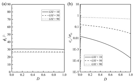
Figure 7.
Influence of D on equivalent MC parameters (β = 45°): (a) equivalent internal friction angle ϕe; (b) equivalent cohesion ce/σci.
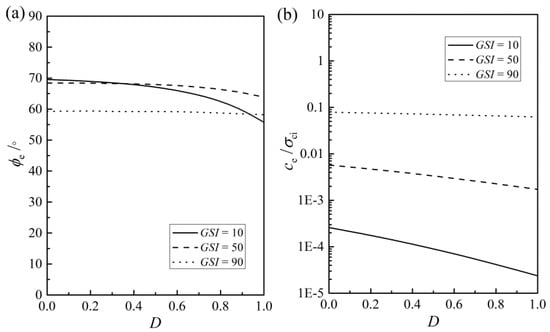
Figure 8.
Influence of D on equivalent MC parameters (β = 90°): (a) equivalent internal friction angle ϕe; (b) equivalent cohesion ce/σci.
3.2. Slope Geometries on Equivalent MC Strengths
As illustrated in these aforementioned results, the equivalent MC strength parameters (ϕe and ce/σci) are quite different for slopes with various inclinations. Hence, Figure 9 presents the influence of inclination angle β on the equivalent MC strength parameters for 3D static slopes in different conditions of nonlinear strengths. The value of the disturbance coefficient D is 0, the value of the constant mi is 10 and 25, and the geological strength index GSI is considered in three conditions: GSI = 10; GSI = 50; GSI = 100. Additionally, the slope relative width B/H is 2.0. As presented in Figure 9, the inclination angle β has a significant influence on the equivalent strength parameters. As β increases, the equivalent friction angle ϕe becomes larger, but the equivalent cohesion ce/σci becomes smaller. As presented in the study of Wu et al. [29], the slope slip surface becomes shallower as the inclination angle β increases. Hence, the normal stresses along the slip surface of steeper slopes will be within a small range. As the inclination angle β increases, the position of the tangent point will move towards the origin, with two equivalent parameters changing in opposite directions. Moreover, the increasing or decreasing trend was found to be more obvious for slopes in rocks with a larger mi value and a smaller GSI value. This reveals that the influence of β on the equivalent MC parameters will be more significant for slopes in fractured rock masses composed of igneous or metamorphic rocks.
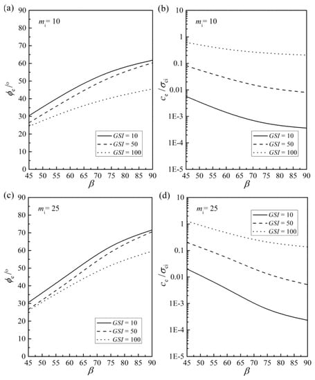
Figure 9.
Influence of β on equivalent MC parameters: (a) equivalent internal friction angle ϕe in case of mi = 10; (b) equivalent cohesion ce/σci in case of mi = 10; (c) equivalent internal friction angle ϕe in case of mi = 25; (d) equivalent cohesion ce/σci in case of mi = 25.
In order to reveal the influence of 3D geometry of the slope on the equivalent MC parameters, Figure 10 gives the curves of the equivalent internal friction angle ϕe for two static slopes with the ratio B/H as the horizontal coordinate. In the figure, four conditions of nonlinear parameters were considered as follows: GSI = 10, mi = 35; GSI = 10, mi = 10; GSI = 100, mi = 35; GSI = 100, mi = 10. In addition, the rock disturbance coefficient D is adopted as 0. From Figure 10, it is obvious that the value of the equivalent internal friction angle ϕe is almost constant with the increasing B/H for different slopes. As shown in Equation (11), the equivalent cohesion ce/σci is an expression of the equivalent internal friction angle ϕe and the expression does not contain B/H. Hence, the value of the equivalent cohesion ce/σci will also remain constant as B/H increases. In other words, although the 3D effect of the slope affects the slope stability, it has no effect on the equivalent MC parameters.
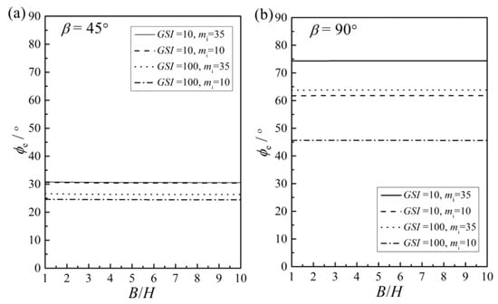
Figure 10.
Influence of B/H on equivalent friction angle ϕe: (a) equivalent internal friction angle ϕe; (b) equivalent cohesion ce/σci.
3.3. Effect of Earthquakes on Equivalent MC Strengths
To illustrate the effect of earthquakes on the equivalent MC strength parameters (ϕe and ce/σci), two kinds of 3D slopes with β = 45° and β = 90° were considered in this section. The slope relative width B/H was assumed as 2.0. The equivalent MC strength parameters were presented by using the seismic coefficient kh as the X-axis in Figure 11 and Figure 12. Similarly, the disturbance coefficient D was adopted as 0. The constant mi and the geological strength index GSI have different values in each figure.
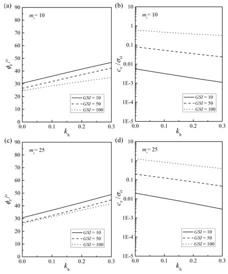
Figure 11.
Influence of kh on equivalent MC parameters (β = 45°): (a) equivalent internal friction angle ϕe in case of mi = 10; (b) equivalent cohesion ce/σci in case of mi = 10; (c) equivalent internal friction angle ϕe in case of mi = 25; (d) equivalent cohesion ce/σci in case of mi = 25.
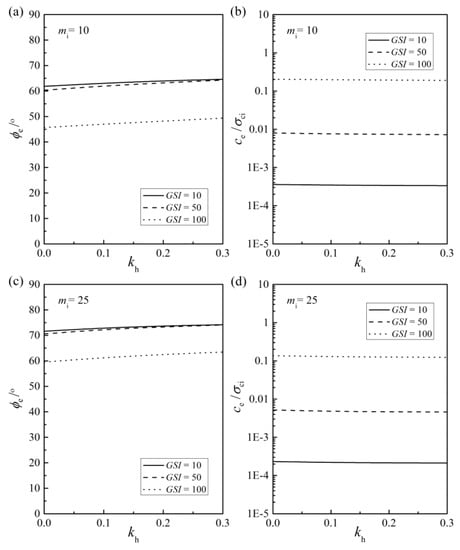
Figure 12.
Influence of kh on equivalent MC parameters (β = 90°): (a) equivalent internal friction angle ϕe in case of mi = 10; (b) equivalent cohesion ce/σci in case of mi = 10; (c) equivalent internal friction angle ϕe in case of mi = 25; (d) equivalent cohesion ce/σci in case of mi = 25.
For rock slopes with β = 45° in Figure 11, the equivalent friction angle ϕe becomes greater with an increase in seismic coefficient kh, and the equivalent cohesion ce/σci will gradually decrease with an increase in kh. The maximum increase in equivalent friction angle ϕe will reach about 59.6%, and the maximum decrease in equivalent cohesion ce/σci will reach about 85.5% for slopes with mi = 25 and GSI = 10. Moreover, the influence of kh on the equivalent parameters ϕe and ce/σci seem to be more obvious for slopes in fractured rock masses (i.e., the value of GSI is smaller). As shown in Figure 12, the equivalent parameters ϕe and ce/σci for vertical slopes (β = 90°) tend to change slightly as the seismic coefficient kh increases. For vertical slopes with the conditions of mi = 25 and GSI = 10, the equivalent friction angle ϕe will increase by about 3.6% and the equivalent cohesion ce/σci will decrease by about 8.3%. This means that the earthquake has a weak influence on the approximate parameters for steep rock slopes. Especially for vertical slopes, the impact of earthquakes on the equivalent parameters may be ignored.
3.4. Approximate MC Parameters Charts
Based on the above analyses, it can be found that the rock material constant mi and the geological strength index GSI have significant effects on the equivalent MC parameters. The influence of disturbance factor D on the equivalent MC parameters should be considered only when the GSI is small. Additionally, the 3D effect of the slope (width-to-height ratio B/H) has almost no effect on the equivalent MC parameters. Therefore, the charts of the equivalent MC parameters (ϕe and ce/σci) for 2D static slopes in undisturbed rock masses (D = 0) were presented in Table 1 and Table 2. For 2D seismic slopes with kh = 0.3, similar charts were also presented in Table 3 and Table 4. It should be noted that the practicable equivalent cohesion ce will be derived when the ratio of ce/σci is multiplied by the uniaxial compressive strength σci. In these tables, the different values of nonlinear strength parameters mi, σci, and GSI were considered by referring to the studies of Hoek and his team [6,7,8,9]. These tabular data can provide some alternative references for the determination of approximate MC parameters in practical slope engineering.

Table 1.
Approximate friction angle ϕe/° for various static slopes.
Table 2.
Approximate cohesion ce/σci for various static slopes.
Table 3.
Approximate friction angle ϕe/° for various rock slopes with kh = 0.3.
Table 4.
Approximate cohesion ce/σci for various rock slopes with kh = 0.3.
4. Conclusions
For 3D rock slopes, the limit analysis method for slope seismic stability with the HB criterion was established. Based on the numerical optimization, the equivalent MC strength parameters were derived for slopes with different nonlinear strengths and geometric characters. Further investigations were made to explore the influences of seismic action, geometric parameters, and nonlinear strengths on the equivalent MC parameters. Approximate MC parameters for reference in practical slope projects were given in some charts. The main conclusions drawn from the research results can be summarized as follows:
(1) The influence laws of rock material constant mi and geological strength index GSI on equivalent MC strength parameters (ϕe and ce/σci) are not in agreement for general steep slopes and vertical slopes. The disturbance factor D has a certain effect on the equivalent MC parameters only for vertical slopes in fractured rock masses. Since the normal stresses on the slope slip surface are in a smaller range as the slope inclination increases, the equivalent strength parameters tend to be more sensitive to the HB strength parameters for vertical slopes.
(2) The slope inclination has significant influences on the equivalent MC strength parameters (ϕe and ce/σci). These effects will become obvious for slopes in fractured rock masses composed of hard rocks. The equivalent MC parameters are slightly affected by the 3D effect of rock slopes, which is represented by the ratio of B/H.
(3) With the increasing seismic load, the equivalent friction angle ϕe increases and the equivalent cohesion ce/σci gradually decreases. The maximum increase in equivalent friction angle ϕe can reach 59.6% and the maximum decrease in equivalent cohesion ce/σci can reach 85.5%. The influence of seismic load on the approximate MC parameters tends to be slight for vertical rock slopes.
Author Contributions
Conceptualization, D.W. and X.C.; methodology, D.W. and X.C.; software, Y.T. and X.M.; validation, D.W., Y.T. and X.C.; formal analysis, Y.T. and X.M.; investigation, Y.T. and X.M.; resources, D.W. and X.C.; data curation, D.W.; writing—original draft preparation, Y.T.; writing—review and editing, D.W. and X.C.; visualization, X.M.; supervision, D.W.; project administration, D.W. and X.C.; funding acquisition, X.C. All authors have read and agreed to the published version of the manuscript.
Funding
This research was funded by the National Natural Science Foundation of China, grant number 52208361; and the Natural Science Foundation of Jiangsu Province, grant number BK20220638.
Institutional Review Board Statement
Not applicable.
Informed Consent Statement
Not applicable.
Data Availability Statement
Conflicts of Interest
The authors declare no conflict of interest. The funders had no role in the design of the study; in the collection, analyses, or interpretation of data; in the writing of the manuscript; or in the decision to publish the results.
References
- Bishop, A.W.; Webb, D.L.; Lewin, P.I. Undisturbed samples of London clay from the Ashford common shaft: Strength-effective stress relationships. Geotechnique 1965, 15, 1–31. [Google Scholar] [CrossRef]
- Hoek, E.; Brown, E.T. Empirical strength criterion for rock masses. J. Geotech. Geoenviron. Eng. 1980, 106, 1013–1035. [Google Scholar] [CrossRef]
- Maksmovic, M. Nonlinear failure envelope for soils. J. Geotech. Eng. 1989, 115, 581–586. [Google Scholar] [CrossRef]
- Baker, R. Nonlinear Mohr envelopes based on triaxial data. J. Geotech. Geoenviron. Eng. 2004, 130, 498–506. [Google Scholar] [CrossRef]
- Anyaegbunam, A. Nonlinear power-type failure laws for geomaterials: Synthesis from triaxial data, properties, and applications. Int. J. Geomech. 2015, 15, 04014036. [Google Scholar] [CrossRef]
- Hoek, E. Strength of jointed rock masses. Geotechnique 1983, 33, 187–223. [Google Scholar] [CrossRef]
- Hoek, E. Estimating Mohr-Coulomb friction and cohesion values from the Hoek-Brown failure criterion. Int. J. Rock Mech. Min. Sci. Geomech. Abstr. 1990, 27, 227–229. [Google Scholar] [CrossRef]
- Hoek, E.; Brown, E.T. Practical estimates of rock mass strength. Int. J. Rock Mech. Min. Sci. 1997, 34, 1165–1186. [Google Scholar] [CrossRef]
- Hoek, E.; Carranza-Torres, C.; Cotkum, B. Hoek-Brown failure criterion-2002 edition. In Proceedings of the NARMS-Tac, Toronto, ON, Canada, 7–10 July 2002; pp. 267–273. [Google Scholar]
- Wei, X.; Zuo, J.; Shi, Y.; Liu, H.; Jiang, Y.; Liu, C. Experimental verification of parameter m in Hoek–Brown failure criterion considering the effects of natural fractures. J. Rock Mech. Geotech. Eng. 2020, 12, 1036–1045. [Google Scholar] [CrossRef]
- Xia, K.; Chen, C.; Wang, T.; Zheng, Y.; Wang, Y. Estimating the geological strength index and disturbance factor in the Hoek–Brown criterion using the acoustic wave velocity in the rock mass. Eng. Geol. 2022, 306, 106745. [Google Scholar] [CrossRef]
- Dawson, E.; You, K.; Park, Y. Strength-reduction stability analysis of rock slopes using the Hoek-Brown failure criterion. Geotech. Special Publication 2000, 290, 65–77. [Google Scholar]
- Yang, X.L.; Li, L.; Yin, J.H. Seismic and static stability analysis for rock slopes by a kinematical approach. Geotechnique 2004, 54, 543–550. [Google Scholar] [CrossRef]
- Li, A.J.; Lyamin, A.V.; Merifield, R.S. Seismic rock slope stability charts based on limit analysis methods. Comput. Geotech. 2009, 36, 135–148. [Google Scholar] [CrossRef]
- Gao, Y.F.; Wu, D.; Zhang, F.; Lei, G.H.; Qin, H.; Qiu, Y. Limit analysis of 3D rock slope stability with non-linear failure criterion. Geomech. Eng. 2016, 10, 59–76. [Google Scholar] [CrossRef]
- Karrech, A.; Dong, X.; Elchalakani, M.; Basarir, H.; Shahin, M.A.; Regenauer-Lieb, K. Limit analysis for the seismic stability of three-dimensional rock slopes using the generalized Hoek-Brown criterion. Int. J. Min. Sci. Technol. 2022, 32, 237–245. [Google Scholar] [CrossRef]
- Londe, P. Discussion of “Determination of the Shear Failure Envelope in Rock Masses” by Roberto Ucar (March, 1986, Vol. 112, No. 3). J. Geotech. Eng. 1988, 114, 374–376. [Google Scholar] [CrossRef]
- Carranze-Torres, C. Elasto-plastic solution of tunnel problems using the generalized form of the Hoek-Brown failure criterion. Int. J. Rock Mech. Min. Sci. 2004, 41, 480–481. [Google Scholar] [CrossRef]
- Fu, W.; Liao, Y. Non-linear shear strength reduction technique in slope stability calculation. Comput. Geotech. 2010, 37, 288–298. [Google Scholar] [CrossRef]
- Chen, Y.; Lin, H. Consistency analysis of Hoek–Brown and equivalent Mohr–coulomb parameters in calculating slope safety factor. Bull. Eng. Geol. Environ. 2019, 78, 4349–4361. [Google Scholar] [CrossRef]
- Renani, H.R.; Martin, C.D. Slope stability analysis using equivalent Mohr–Coulomb and Hoek–Brown criteria. Rock Mech. Rock Eng. 2020, 53, 13–21. [Google Scholar] [CrossRef]
- Yang, X.L.; Yin, J.H. Linear Mohr-Coulomb strength parameters from the non-linear Hoek-Brown rockmasses. Int. J. Non-Linear Mech. 2006, 41, 1000–1005. [Google Scholar] [CrossRef]
- Shen, J.; Priest, S.D.; Karkus, M. Determination of Mohr-Coulomb shear strength parameters from generalized Hoek-Brown criterion for slope stability analysis. Rock Mech. Rock Eng. 2012, 45, 123–129. [Google Scholar] [CrossRef]
- Ren, J.; Chen, X.; Wang, D.; Lv, Y. Instantaneous linearization strength reduction technique for generalized Hoek-Brown criterion. Rock Soil Mech. 2019, 12, 1–8. (In Chinese) [Google Scholar]
- Zhao, L.; Cheng, X.; Li, L.; Chen, J.; Zhang, Y. Seismic displacement along a log-spiral failure surface with crack using rock Hoek–Brown failure criterion. Soil Dyn. Earthq. Eng. 2017, 99, 74–85. [Google Scholar] [CrossRef]
- Pang, Z.; Gu, D. Seismic stability of a fissured slope based on nonlinear failure criterion. Geotech. Geol. Eng. 2019, 37, 3487–3496. [Google Scholar] [CrossRef]
- Zhong, J.H.; Yang, X.L. Pseudo-dynamic stability of rock slope considering Hoek–Brown strength criterion. Acta Geotech. 2022, 17, 2481–2494. [Google Scholar] [CrossRef]
- Shen, J.; Karakus, M. Three-dimensional numerical analysis for rock slope stability using shear strength reduction method. Can. Geotech. J. 2014, 51, 164–172. [Google Scholar] [CrossRef]
- Wu, D.; Gao, Y.; Chen, X.; Wang, Y. Effects of soil strength nonlinearity on slip surfaces of homogeneous slopes. Int. J. Geomech. 2021, 21, 06020035. [Google Scholar] [CrossRef]
- Wu, D.; Shen, F. Stability assessment of coastal clay slopes considering strength nonlinearity and sea level drawdown. Mar. Georesour. Geotec. 2022, 2022, 1–17. [Google Scholar] [CrossRef]
- Li, X. Finite element analysis of slope stability using a nonlinear failure criterion. Comput. Geotech. 2007, 34, 127–136. [Google Scholar] [CrossRef]
- Michalowski, R.L.; Drescher, A. Three-dimensional stability of slopes and excavations. Geotechnique 2009, 59, 839–850. [Google Scholar] [CrossRef]
- Gao, Y.F.; Zhang, F.; Lei, G.H.; Li, D.Y. An extended limit analysis of three-dimensional slope stability. Geotechnique 2013, 63, 518–524. [Google Scholar] [CrossRef]
- Xu, J.; Pan, Q.; Yang, X.L.; Li, W. Stability charts for rock slopes subjected to water drawdown based on the modified nonlinear Hoek-Brown failure criterion. Int. J. Geomech. 2018, 18, 04017133. [Google Scholar] [CrossRef]
- Michalowski, R.L.; Park, D. Three-dimensional ridge collapse mechanism for narrow soil slopes. Int. J. Numer. Anal. Methods Geomech. 2021, 45, 1972–1987. [Google Scholar] [CrossRef]
- Pan, Q.; Zhang, R.; Wang, S.; Chen, J.; Zhang, B.; Zou, J.; Yang, X. Three-dimensional stability of slopes under water drawdown conditions. Int. J. Geomech. 2023, 23, 04022254. [Google Scholar] [CrossRef]
- Michalowski, R.L.; Martel, T. Stability charts for 3D failures of steep slopes subjected to seismic excitation. J. Geotech. Geoenviron. Eng. 2011, 137, 183–189. [Google Scholar] [CrossRef]


Disclaimer/Publisher’s Note: The statements, opinions and data contained in all publications are solely those of the individual author(s) and contributor(s) and not of MDPI and/or the editor(s). MDPI and/or the editor(s) disclaim responsibility for any injury to people or property resulting from any ideas, methods, instructions or products referred to in the content. |
© 2023 by the authors. Licensee MDPI, Basel, Switzerland. This article is an open access article distributed under the terms and conditions of the Creative Commons Attribution (CC BY) license (https://creativecommons.org/licenses/by/4.0/).