Site Characterization and Liquefaction Hazard Assessment for the Erenler Settlement Area (Sakarya Province, Turkey) Based on Integrated SPT-Vs Data

Abstract

The focus of this study is to examine the soil properties and liquefaction potential of the Erenler center district in a critical tectonic zone that can produce large earthquakes, such as the North Anatolian Fault Zone (NAFZ). In this sense, 40 surface wave measurements and 52 geotechnical drillings were employed. Accordingly, the liquefaction potential index (LPI), liquefaction severity index (LSI), Ishihara boundary (IB) curve, and Ishihara-inspired index (LPI_ISH) liquefaction approaches from geotechnical and geophysical methods were used as integrated. All liquefaction analyses were examined for two scenarios, Mw: 7.4 1999 Izmit (a_max: 0.41 g) and Mw: 7.0 1967 (a_max: 0.28 g) Mudurnu. According to the analyses, almost all of the study area showed liquefaction risk in the Izmit scenario. In the Mudurnu scenario, liquefaction risk distribution decreased parallel to acceleration. The LPI, LPI_ISH, and IB liquefaction risk results for both scenarios support each other. On the other hand, it was determined that the probability of liquefaction was lower in the LSI evaluation. The spatial distribution of the liquefaction potential of the Vs-based and SPT-based LPI assessments had a similar pattern. These results show that the LPI approach, originally SPT-based, can also be calculated based on Vs. In addition, according to Vs₃₀-based (average shear wave velocity at 30 m depth) soil classification criteria, low-velocity character E and D soil groups dominate the Quaternary alluvial basin. This indicates that deformation-induced failures may occur even in areas with a low probability of liquefaction in similar strong ground motions. In addition, the evaluation of liquefaction with many approaches in two different bases within the scope of the study constitutes a novelty for the study area and liquefaction analyses. While performing diversified liquefaction analyses and approaches will contribute to obtaining more reliable soil liquefaction results, more case studies are needed to elucidate these comparisons.

1. Introduction

One of the causes of natural disasters after an earthquake is the effects of collapse and deformations resulting from liquefaction with the impact of cyclic stress loads. As known, in the case of liquefaction, with the excessive increase in pore water pressure, the effective stress will converge to a very low value, and the soil will lose its bearing strength. Thus, loading forces cause failures, especially in engineering structures, and can cause deformation or failure for infrastructure systems, the collapse of buildings, and undesirable situations in fuel storage facilities. The first findings regarding assessing liquefaction potential were offered by Seed and Idriss [1] after the 1964 Alaska and Niigata earthquakes. In this context, many geotechnical approaches have been presented in the following years to examine this problem according to SPT-N values [2,3,4]. Seed and Idriss [1] used the observations from triaxial compression and shear tests to analyze the potential liquefaction of soft saturated sandy soils. Seed and Idriss [3] correlated the cyclic stress ratio (CSR) and the corresponding SPT-N values of the samples for both liquefied and non-liquefied layers. Then, they developed the safety factor (FS) for soil liquefaction potential by using the cyclic stress ratio (CSR) and cyclic resistance ratio (CRR) [3]. Afterward, Seed et al. [5] revised the CSR to consider the effect of shear stresses and effective overburden pressure. In conclusion, many researchers have used this liquefaction analysis until today [4,6,7,8].

Because the shear wave velocity can also be used to determine the cyclic shear stress of the soil, liquefaction analyses based on shear wave velocity have found a place in the literature with Dobry et al. [9], following the shape of geotechnical approaches. Robertson [10] considered it necessary to correct the shear wave velocity in the liquefaction analysis with effective stress. Andrus and Stoke II [11] calculated the CRR from the shear wave velocity and revealed the relationship between the CRR and the corrected shear wave velocity. Kayen et al. [12] developed a new CRR correlation that directly considers earthquake magnitude, ground acceleration, corrected shear wave velocity, and critical layer depth. With the approaches using this corrected shear wave velocity, the liquefaction assessment is widely applied to the calculation of the FS, just as in the SPT-N assessment [13,14,15].

Iwasaki et al. [16,17] stated that it is insufficient to evaluate the liquefaction phenomenon only depending on the FS. They suggested a classification consisting of four categories called the liquefaction potential index (LPI) for liquefaction severity. Afterward, Chen and Juang [18] developed a probability of liquefaction (PL) function based on FS, demonstrating the possibility of soil liquefaction. Juang et al. [19] normalized this parameter and proclaimed a new version varying between values of 0 and 1. Lee et al. [20] suggested the liquefaction risk index (IR) based on the PL with a similar classification as Iwasaki et al. [17]. Sonmez and Gokceoglu [21] argued that the classification ranges of Iwasaki et al. [17] and Lee et al. [20] are narrow. Hence, they revealed a liquefaction severity index (LSI), including more classes ranging from 1 to 100 [21]. This satisfactory classification is widely used [22,23]. However, these indices determine the liquefaction potential of the entire soil profile. Therefore, whether the surface damage of the liquefiable layers will occur in possible earthquakes can be checked by the Ishihara boundary (IB) curve [24]. Maurer et al. [25] suggested the calibration of LPI values with an exponential depth weight function, including the effect of the thickness of the non-liquefiable surface layers on surface liquefaction. This approach is defined as the Ishihara-inspired index (LPI_ISH) and controls surface liquefaction.

Turkey, in the Alpine–Himalayan orogenesis, is exposed to quite large earthquakes due to its tectonic zones. The North Anatolian Fault Zone (NAFZ), which starts from the Karliova triple junction and extends approximately 1500 km to the west, plays a central role in this earthquake activity. The 1999 Izmit, Duzce, and the 1967 Mudurnu earthquakes, which severely affected the study area and its surroundings, are the most significant earthquakes in the west branch of the NAFZ in the last 60 years (Figure 1). Especially in the studies performed after the Izmit earthquake, it was emphasized that the soil liquefaction triggered the building damage. For this reason, the Sakarya region, a natural laboratory in terms of liquefaction, has been an important data source for theoretical liquefaction studies [26,27,28]. The mentioned liquefaction assessment studies after the earthquake focused on the central Adapazari region and were limited to plot-based studies in some parts of the Sapanca district [29]. The Erenler center settlement, located on alluvial deposits formed by the Sakarya River, is characterized by sandy-silty-clayey units and shallow underground levels. As expected, joining sandy units with near-surface groundwater levels under large-magnitude earthquakes considerably increases the risk of liquefaction in the study area.

The main goal of this study is to evaluate the soil properties and the potential liquefaction risk of the Erenler center district by using the surface wave method and geotechnical approaches. Thus, an innovative liquefaction assessment based on two different field data obtained by geotechnical and geophysical methods was achieved for the study area. In this context, the liquefaction potential of the study area was evaluated according to the 1999 Izmit and 1967 Mudurnu earthquake scenarios, destructive to the study area, using 52 boreholes and 40 surface wave analyses. In SPT-N-based analysis, LPI, LPI_ISH and LSI liquefaction classification indexes were used to define the liquefaction hazard by calculating FS values. Surface damage presence after liquefaction was checked by the IB curve. The Vs-based liquefaction analysis was performed according to the approach by Kayen et al. [12]. The results of the methods were visualized in the GIS environment with surface distribution maps using the inverse distance interpolation technique and were examined in detail.

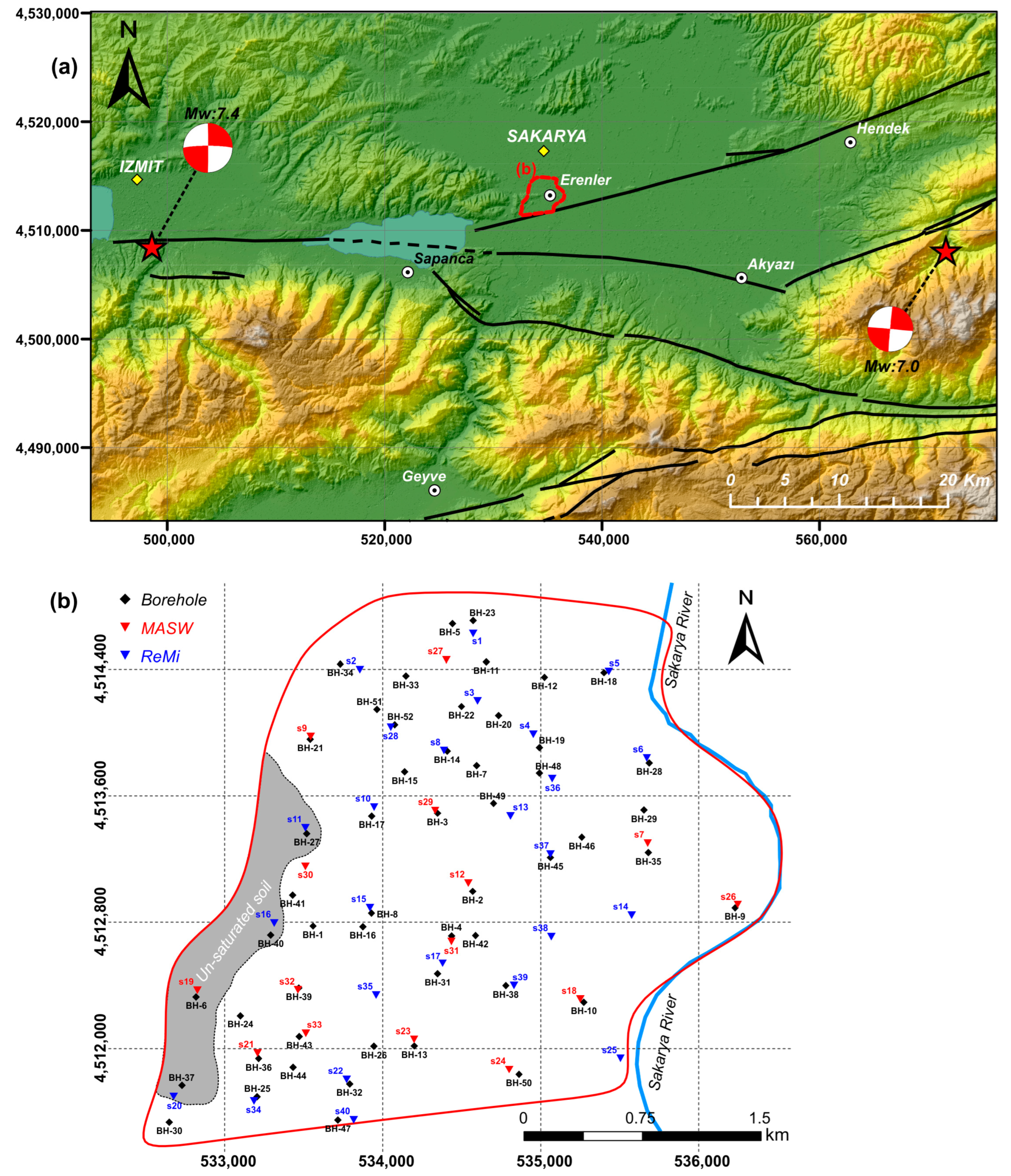
2. Geological and Tectonic Features

The Marmara region is located in the western extension of the North Anatolian Fault Zone, one of Turkey’s and the world’s most critical strike-slip zones. After entering the Marmara region, the NAFZ divides into three branches (north-mid-south) in eastern Marmara [32]. GPS measurements reveal that the northern branch is more active than the other branches, with a fault slip rate of 22 ± 3 mm/yr) [33]. Sakarya and its vicinity, located between the Samanlı Mountains in the north and the Kocaeli peneplain, have been exposed to many earthquakes Ms ≥ 6.8 in both historical and instrumental periods due to this tectonic characteristic on the more active northern branch [34]. This activity can also be seen in the seismicity map of the last century (Figure 1). The Erenler settlement center is located between the pull-apart Sapanca basin, formed by the strike-slip mechanism of the NAFZ, and the Sakarya river. On the other hand, the fault rupture during the 1999 Izmit earthquake occurred towards the study area with the 3–4.5 m lateral slips [35] measured in the Sapanca-Akyazı segment located within the boundaries of Erenler necessitated a risk assessment for the study area.

A general geological map of the study area and its immediate surroundings is illustrated in Figure 1c. In this map, the geological formations are listed as Akveren, Yığılca, Çaycuma, Örencik, alluvial fan and alluvium from the oldest to the youngest. Among these units, the Akveren formation and alluvial units consisting of lateral-vertical transitional fluvial deposits of the Sakarya River are included in the study (Figure 1c). The Akveren formation, an outcropping in the west of the study area boundary, is Upper Cretaceous–Lower Eocene aged. It consists of clayey limestone, marl, claystone, siltstone, sandstone, conglomerate, and reef limestone units. A large part of the Erenler settlement area formed by the Sakarya River consists of Quaternary alluvium. These young Quaternary units dominate the propagation of seismic waves and the amplitude of strong ground motion. This unit consists of gravel, sand, silt, clay, and their combinations at different depths under the influence of the sediments carried and deposited by the Sakarya river located on the eastern border of the study area [31]. In this geological regime, the distribution of groundwater varies in the range of 1–3.5, which is quite shallow throughout the study area.

3. Liquefaction Approaches

3.1. Earthquake Selection and PGA Estimation

The immediate surroundings of the study area have intense seismic activity arising from the NAFZ. The NAFZ is divided into north and south branches in the Eastern Marmara region, where the study area is located. Ground acceleration produced by earthquakes is another critical parameter in the liquefaction assessment for the study area. In this study, the 1999 Izmit (Mw: 7.4) and 1967 Mudurnu (Mw: 7.0) earthquakes, which occurred on the eastern and western segments of the study area, were preferred as a scenario earthquake to evaluate the liquefaction potential (Figure 2).

These earthquakes produce effective surface rupture and displacement [35]. The maximum horizontal ground acceleration (a_max) in the 1999 Izmit earthquake was measured as 0.41 g [26] at the 5401 Sakarya station. This value was used in this study. There are no such numerical data for the 1967 earthquake, which occurred approximately 38 km (R) from the study area. Various empirical approaches consider the fault and soil properties for determining a_max in such cases. In this study, the a_max for the 1967 Mudurnu earthquake was calculated as 0.28 g using the Graizer and Kalkan [36] equation (Figure 3).

3.2. Liquefaction Probability Based on SPT-N

There are different geotechnical approaches for the assessment of liquefaction potential. The most widespread method is the simplified liquefaction approach proposed by Seed and Idriss [1] after the 1964 Niigata and Alaska earthquakes. This method gives the FS based on the ratio between cyclic resistance (CRR) and cyclic stress (CSR). In this study, a probabilistic-deterministic approach developed by Cetin et al. [6] and updated with new case history data by Cetin et al. [8] was used for the liquefaction analysis. In this approach, the equation given by CSR, Seed and Idriss [1] is used as follows:

$${\mathrm{CSR}}_{{\mathsf{\sigma }}_{\mathrm{v}}^{\prime },{\mathrm{M}}_{\mathrm{w}}}=0.65\left(\frac{{\mathrm{a}}_{\max }}{\mathrm{g}}\right)\left(\frac{{\mathsf{\sigma }}_{\mathrm{v}}}{{\mathsf{\sigma }}_{\mathrm{v}}^{\prime }}\right){\mathrm{r}}_{\mathrm{d}}$$

(1)

where ${\mathrm{a}}_{\max }$ is the maximum horizontal ground acceleration on the surface, $\mathrm{g}$ is the acceleration due to gravity, ${\mathsf{\sigma }}_{\mathrm{v}0}$ and ${\mathsf{\sigma }}_{\mathrm{v}0}^{\prime }$ are the vertical total and effective stresses, and ${\mathrm{r}}_{\mathrm{d}}$ is the stress reduction coefficient. Here, is rd calculated with Equation (2) developed by Cetin and Seed [37], based on shear wave velocity (Vs):

$${\mathrm{r}}_{\mathrm{d}}\left(\mathrm{d},{\mathrm{M}}_{\mathrm{w}},{\mathrm{a}}_{\max },{\mathrm{V}}_{\mathrm{s},12}^{\ast }\right)=\frac{\left[1+\frac{-23.013-2.949{\times \mathrm{a}}_{\max }+0.999{\times \mathrm{M}}_{\mathrm{w}}+0.0525{\times \mathrm{V}}_{\mathrm{s},12}^{\ast }}{16.258+0.201{\times \mathrm{e}}^{0.341\left(-\mathrm{d}+0.0785{\times \mathrm{V}}_{\mathrm{s},12}^{\ast }+7.586\right)}}\right]}{\left[1+\frac{-23.013-2.949{\times \mathrm{a}}_{\max }+0.999{\times \mathrm{M}}_{\mathrm{w}}+0.0525{\times \mathrm{V}}_{\mathrm{s},12}^{\ast }}{16.258+0.201{\times \mathrm{e}}^{0.341\left(0.0785{\times \mathrm{V}}_{\mathrm{s},12}^{\ast }+7.586\right)}}\right]\pm {\mathsf{\sigma }}_{{\mathsf{\epsilon }}_{{\mathrm{r}}_{\mathrm{d}}}}}$$

(2)

where d and ${\mathrm{V}}_{\mathrm{s},12}^{\ast }$ represent the depth with d < 20 m and average share wave velocity for the upper 12.2 m soil profile, respectively. The term ${\mathsf{\sigma }}_{{\mathsf{\epsilon }}_{{\mathrm{r}}_{\mathrm{d}}}}$ designates the standard deviation of the model correction term, and Mw is the moment magnitude. The Vs values in this study are based on actual field measurements rather than empirical correlations. Fine content (FC) correction for the SPT-N values by Cetin et al. [8] was performed using Equation (3), as follows:

$${\mathrm{N}}_{1,60,\mathrm{CS}}={\mathrm{N}}_{1,60}+\mathrm{FC}\times \left(0.00167{\times \mathrm{N}}_{1,60}+0.089\right)$$

(3)

where ${\mathrm{N}}_{1,60}$ is the corrected blow count and ${\mathrm{N}}_{1,60,\mathrm{cs}}$ is the fine content corrected blow count. In the calculation of CRR, Cetin et al. [8] proposed the following pair of equations with the recent model coefficients.

$${\mathrm{P}}_{\mathrm{L}}\left({\mathrm{N}}_{1,60},{\mathrm{CSR}}_{{\mathsf{\sigma }}_{\mathrm{v}}^{\prime },\mathsf{\alpha }=0,{\mathrm{M}}_{\mathrm{w}}}{\mathrm{M}}_{\mathrm{w}},{\mathsf{\sigma }}_{\mathrm{v}}^{\prime },\mathrm{FC}\right)=\mathsf{\Phi }\left[-\frac{\left(\begin{array}{c}{\mathrm{N}}_{1,60}\times \left(1+0.00167\times \mathrm{FC}\right)-11.771\times \mathrm{l}\mathrm{n}\left({\mathrm{CSR}}_{{\mathsf{\sigma }}_{\mathrm{v}}^{\prime },\mathsf{\alpha }=0,{\mathrm{M}}_{\mathrm{w}}}\right)\\ -27.352\times \mathrm{l}\mathrm{n}\left({\mathrm{M}}_{\mathrm{w}}\right)-3.958\times \mathrm{l}\mathrm{n}\left(\frac{{\mathsf{\sigma }}_{\mathrm{v}}^{\prime }}{{\mathrm{P}}_{\mathrm{a}}}\right)+0.089\times \mathrm{F}\mathrm{C}+16.084\end{array}\right)}{2.95}\right]$$

(4)

$$\mathrm{CRR}\left({\mathrm{N}}_{1,60},{\mathrm{M}}_{\mathrm{w}},{\mathsf{\sigma }}_{\mathrm{v}}^{\prime },\mathrm{FC},{\mathrm{P}}_{\mathrm{L}}\right)=\exp \left[\frac{\left(\begin{array}{c}{\mathrm{N}}_{1,60}\times \left(1+0.00167\times \mathrm{FC}\right)-27.352\times \mathrm{l}\mathrm{n}\left({\mathrm{M}}_{\mathrm{w}}\right)\\ -3.958\times \mathrm{l}\mathrm{n}\left(\frac{{\mathsf{\sigma }}_{\mathrm{v}}^{\prime }}{{\mathrm{P}}_{\mathrm{a}}}\right)+0.089\times \mathrm{F}\mathrm{C}+16.084+2.95\times {\mathsf{\Phi }}^{-1}\left({\mathrm{P}}_{\mathrm{L}}\right)\end{array}\right)}{11.771}\right]$$

(5)

In the given equations, P_L is the probability of liquefaction, ${\mathrm{CSR}}_{{\mathsf{\sigma }}_{\mathrm{v}}^{\prime },\mathsf{\alpha }=0,{\mathrm{M}}_{\mathrm{w}}}$ is the unadjusted value from the vertical effective stress, P_a is atmospheric pressure (100 kPa), and Φ is the standard cumulative normal distribution. The ${\mathsf{\Phi }}^{-1}\left({\mathrm{P}}_{\mathrm{L}}\right)$ function is the inverse of the standard cumulative normal distribution. Cetin et al. [8] graphed the CSR-${\mathrm{N}}_{1,60,\mathrm{CS}}$ values versus different P_L curves. They stated that as a result of these evaluations, the 50% probability curve is more suitable for the liquefaction threshold value of 1.0. Accordingly, CSR-${\mathrm{N}}_{1,60,\mathrm{CS}}$ values for the scenario earthquakes of this study are plotted for different P_L curves (Figure 4).

It is seen in Figure 4 that among the 5%, 50%, and 95% curves, the P_L= 50% curve is more compatible with the calculated values from the boreholes. Finally, the FS value, which allows the liquefaction assessment of the critical layers, was calculated with the following equation:

$$\mathrm{FS}=\frac{{\mathrm{CRR}}_{\left({\mathrm{P}}_{\mathrm{L}}=50\%\right)}}{{\mathrm{CRR}}_{\left({\mathrm{P}}_{\mathrm{L}}\right)}}=\exp [-0.251{\times \mathsf{\Phi }}^{-1}\left({\mathrm{P}}_{\mathrm{L}}\right)]$$

(6)

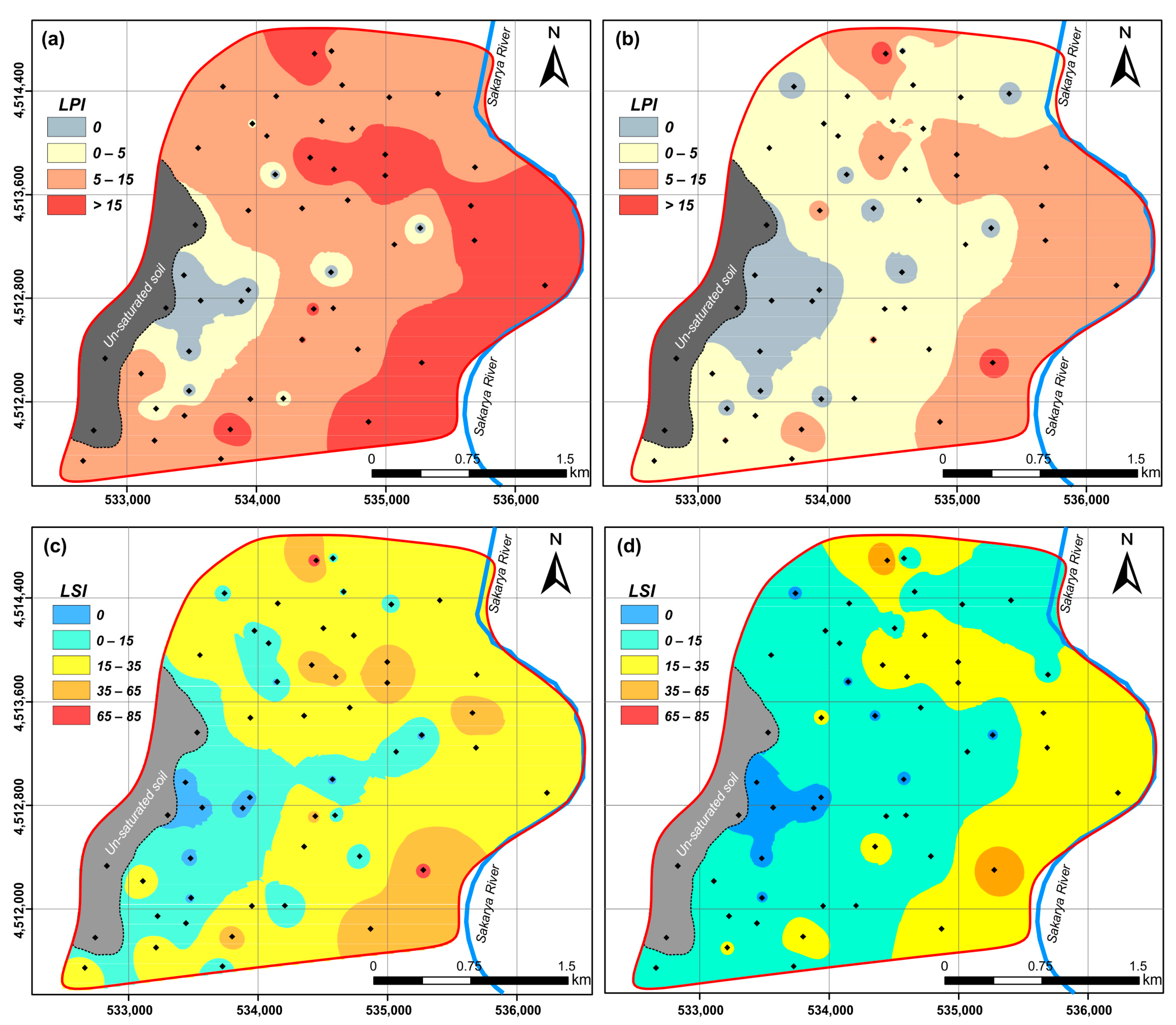
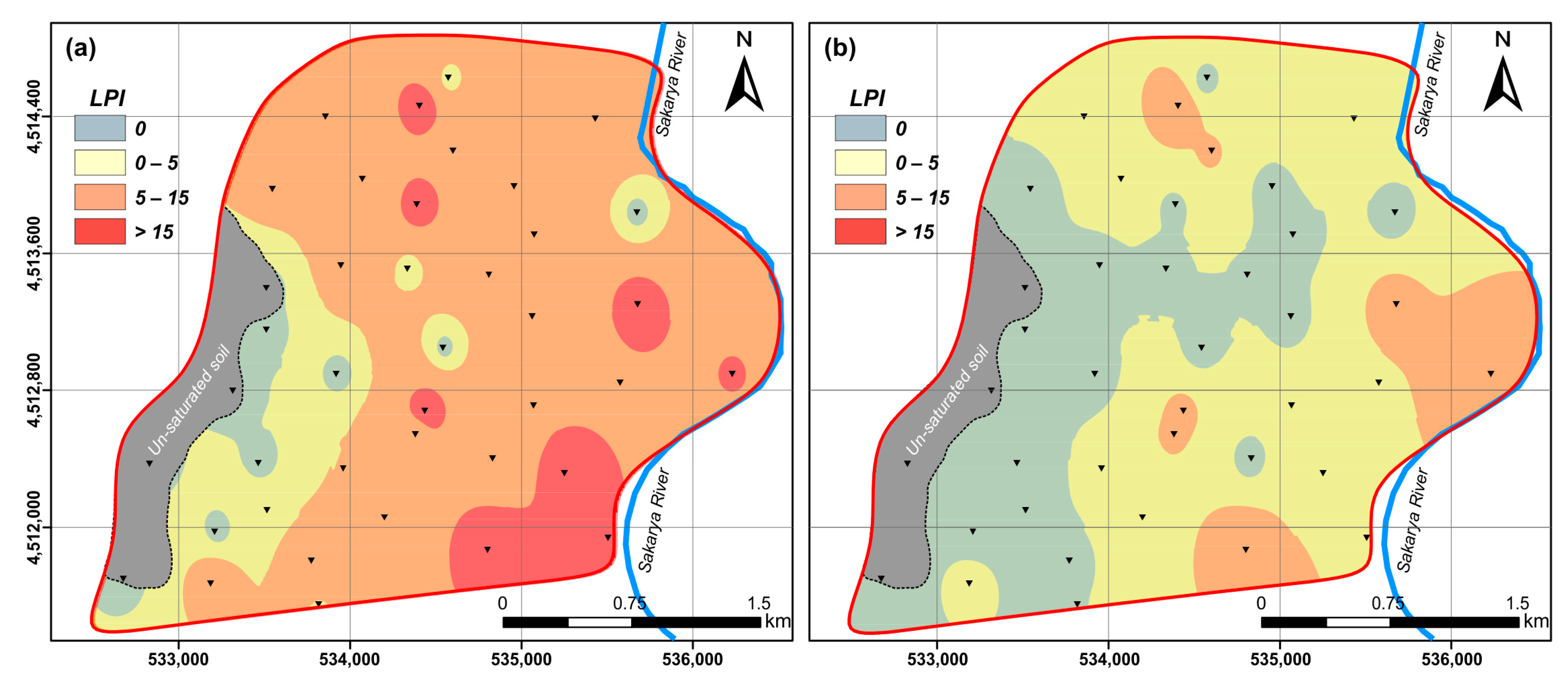
3.2.1. Liquefaction Potential Index (LPI)

Iwasaki et al. [16] emphasized that structural damage significantly depended on the severity of liquefaction and the location of the liquefiable layer at the depth (shallow liquefaction is more damaging than deep liquefaction). They suggested the LPI, which expresses the severity of liquefaction. This approach performs a liquefaction evaluation for the entire soil profile at a depth of 20 m. For the liquefaction potential index, Iwasaki et al. [16] use the following equation:

$$\mathrm{LPI}={{\displaystyle \int }}_0^{20 \mathrm{m}}\mathrm{F}\left(\mathrm{z}\right)\mathrm{W}\left(\mathrm{z}\right)\mathrm{dz}$$

(7)

where F is the function of the safety factor; $\mathrm{F}=0$ for $\mathrm{FS}\ge 1,$ and $\mathrm{F}=1-\mathrm{FS}$ for FS < 1. W is the weight function that depends on depth. $\mathrm{W}=10-0.5\mathrm{z}$ for $\mathrm{z}\le 20 \mathrm{m}$, and $\mathrm{W}=0$ for $\mathrm{z}>20 \mathrm{m}$, where z represents the middle of the soil layer. Iwasaki et al. [17] used the assessment of liquefaction potential into four categories: very low for $\mathrm{LPI}=0$, low for $0<\mathrm{LPI}\le 5$, high for $5<\mathrm{LPI}\le 15$, and very high for $\mathrm{LPI}>15$. The SPT-based LPI method has been used in many case studies to bring out local-regional liquefaction maps based on an entire assessment of the soil profile [38,39,40].

3.2.2. Liquefaction Severity Index (LSI)

Sonmez and Gokceoglu [21] proposed a liquefaction severity index (LSI) with different classification conditions using the liquefaction potential (P_L) index because of the narrow band in LPI classification. In this approach, they defined the liquefaction threshold boundary as $\mathrm{FS}=1.411$. The ${\mathrm{P}}_{\mathrm{L}}$ was calculated for the desired depth with Juang et al. [19] coefficients in the case of $\mathrm{FS}\le 1.411$, and it was regarded as 0 while $\mathrm{FS}>1.411$. The liquefaction severity index (LSI) equation is given as follows:

$$\mathrm{LSI}={{\displaystyle \int }}_0^{20 \mathrm{m}}{\mathrm{P}}_{\mathrm{L}}\left(\mathrm{z}\right)\left(10-0.5\mathrm{z}\right)\mathrm{dz}$$

(8)

where z denotes depth. The LSI assessment is established at six levels: non-liquefiable for $\mathrm{LSI}=0$, very low for $0<\mathrm{LSI}<15$, low for $15\le \mathrm{LSI}<35$, moderate for $35\le \mathrm{LSI}<65$, high for $65\le \mathrm{LSI}<85$, and very high for $85\le \mathrm{LSI}<100$.

3.2.3. Ishihara Boundary Curve (IB)

Ishihara’s boundary criteria [24] examined the effect of non-liquefied soil layers on liquefaction failures at the surface based on field data from earthquakes in China and Japan. While discussing this effect, he emphasized that the thickness of the non-liquefiable surface layers (cap soil) (H₁) is the main factor in the surface damage caused by the liquefied layers (H₂). These mentioned failures are mainly based on surface sand boilings. The a_max controls the boundary curve for the presence of liquefaction-induced surface damage. The Ishihara method is frequently used to evaluate the effects of liquefaction on the ground [41,42,43].

3.2.4. Ishihara-Inspired Index (LPI_ISH)

Maurer et al. [25] emphasized that the LPI index produced consistent results in determining the surface effects of liquefaction, but the LPI values were overestimated compared to actual case data. They suggested an exponential depth weight function inspired by IB curves for LPI values in this context. The LPI_ISH index, which improves the overestimated LPI prediction, is expressed by the following equations.

$${\mathrm{LPI}}_{\mathrm{ISH}}={{\displaystyle \int }}_{{\mathrm{H}}_1}^{20\mathrm{m}}\mathrm{F}\left(\mathrm{FS}\right)\frac{25.56}{\mathrm{z}}\mathrm{dz}$$

(9)

where

$$\mathrm{F}\left(\mathrm{FS}\right)=\{\begin{array}{c}1-\mathrm{F}\mathrm{S} \mathrm{i}\mathrm{f} \mathrm{F}\mathrm{S}\le 1 {\displaystyle \cap } {\mathrm{H}}_1\times \mathrm{m}\left(\mathrm{FS}\right)\le 3\\ 0 \mathrm{o}\mathrm{t}\mathrm{h}\mathrm{e}\mathrm{r}\mathrm{w}\mathrm{i}\mathrm{s}\mathrm{e}\end{array}$$

(10)

$$\mathrm{m}\left(\mathrm{FS}\right)=\exp \left(\frac{5}{25.56\times \left(1-\mathrm{FS}\right)}\right)-1$$

(11)

where z and H₁ are the depth from the surface and the cap soil depth, respectively. In this approach, the threshold value for the liquefaction manifestation is ≥5. In the case studies, the positive contributions of the index are highlighted in the literature [42,44,45].

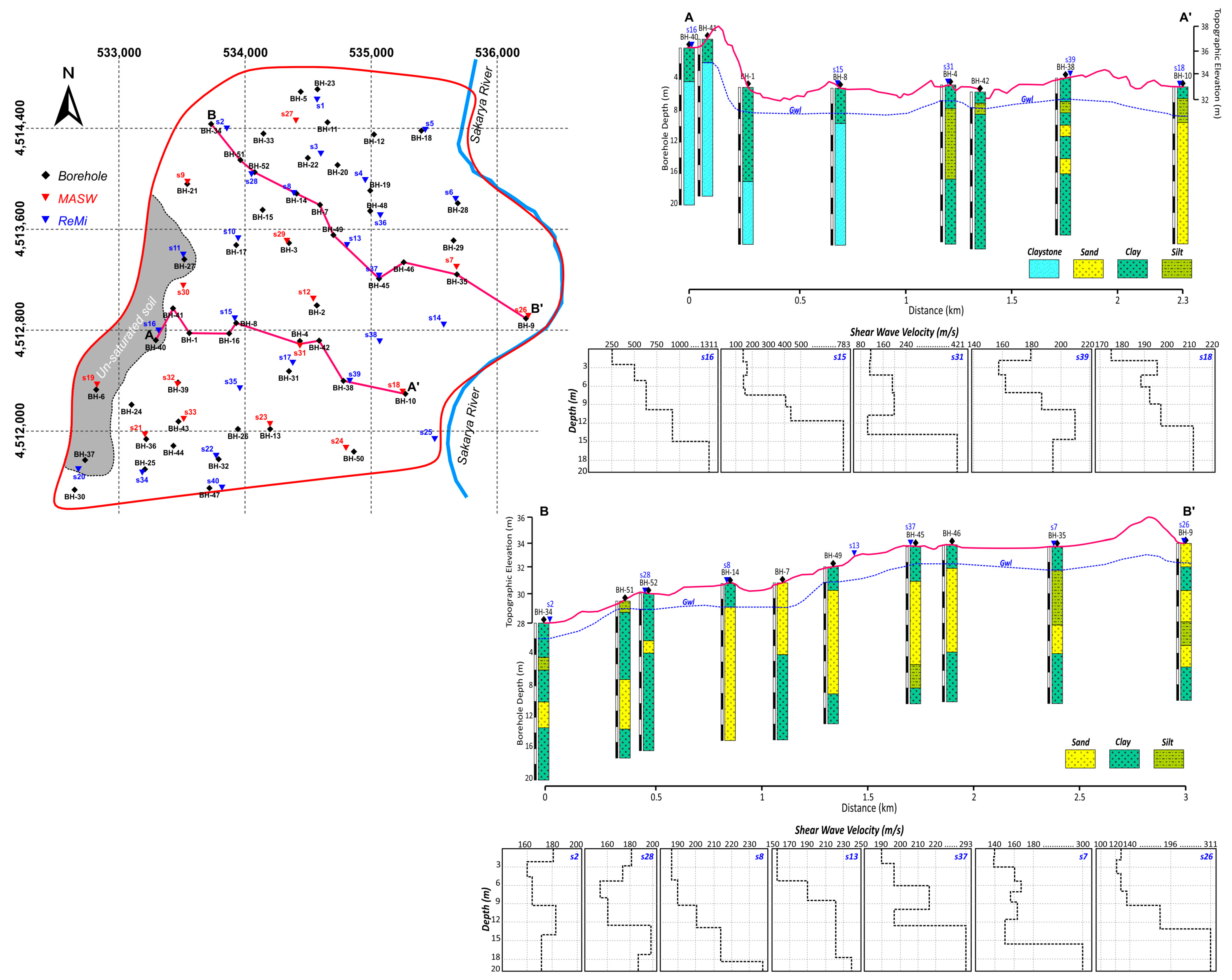
3.3. Shear Wave-Based Liquefaction Analysis

As mentioned, SPT-N counts acquired in geotechnical soil drillings are very common in the deterministic calculation of liquefaction analysis. However, the SPT test is inconsistent in some cases, such as gravelly soils and areas where drilling is impossible. The CSR obtained from the SPT-N numbers is affected by the soil stiffness, groundwater level, density, stress history, etc. Similarly, shear wave velocity is also directly affected by these parameters. This makes it possible to use Vs in liquefaction analysis [12,13].

The simplified liquefaction analysis procedure introduced by Seed and Idriss [1] was applied by Dobry et al. [9] in laboratory conditions with shear waves. In the last 40 years, different approaches have been derived to evaluate liquefaction resistance by shear wave analysis [5,10,11,12,13,15]. These studies focus on calculating the CRR and CSR from the shear wave velocity. In this study, the equations developed by Kayen et al. [12] were used to determine the liquefaction resistance under seismic loads.

3.3.1. Surface Wave Data Acquisition

In this study, multi-channel analysis of surface wave (MASW) [46] and refraction-microtremor (ReMi) [47] methods were used at 40 data measurement locations (Figure 2). Both techniques are widely used to reveal the geotechnical features of the ground [48,49,50]. MASW was used with an active source in this study, while ReMi was used with a passive source. The surface wave analysis is carried out in three steps for both methods. The first step is to acquire data in the time-distance (x-t) domain with the roadside survey array. In both methods, pre-data processing is performed before the second step, which is the design of the dispersion curves. While gain recovery, bandpass filtering (2–44 Hz), and muting were applied in pre-data processing for the MASW process, only gain recovery was implemented in ReMi records. Dispersion analysis in the MASW method is executed by converting the data from the x-t domain to the frequency-phase velocity domain with the wavefield transform method [46,51]. The ReMi method separates Rayleigh waves from other waves by converting the data to the slowness-frequency domain (p-f) with the p-tau transform. Then, the dispersion curve is obtained as described by Thorson and Claerbout [52]. Finally, the dispersion curves were inverted using the least-squares approach, and 1D Vs-depth profiles were created.

The shallow soil properties of the ground are based on the first 30 m of the soil profile in various earthquake codes (National Earthquake Hazards Reduction Program (NEHRP), International Building Code (IBC), Eurocode 8 (EC-8)). On the other hand, the risk of liquefaction is possible up to a maximum depth of 20 m. In this context, 15 MASW and 25 ReMi measurements (Figure 2) were performed to analyze both criteria for the soil profile at a depth of at least 30 m in the study area. For this reason, data acquisition parameters were selected to model at least this depth level and thin layers. Accordingly, data acquisition parameters were set by considering the optimum data acquisition parameters given by Park et al. [53] for the MASW method and by Louie [47,54] for the ReMi method to analyze all these conditions. These data acquisition parameters for the study are given in

Table 1. Data acquisition parameters used in surface wave analysis.

Method	Masw	ReMi
Number of channels	24	24
Sample rate (ms)	0.5	2
Record length (sec)	1	30
Receiver spacing (m)	3	3
Minimal offset (m)	12	-
Array length (m)	72	69
Geophone frequency (Hz)	4.5	4.5
Number of stacks	8–10	8–10
Source	10 kg sledgehammer	Ambient noise

.

3.3.2. Liquefaction Analysis

Analyzing soil liquefaction with the shear wave according to soil conditions and earthquake parameters is possible by calculating three parameters: CSR, CRR, and FS [15]. The FS is represented by the CRR/CSR, similar to the SPT-N analysis. Kayen et al. [12] calculated the cyclic stress ratio due to seismic earthquake loads at the underlying liquefiable strata with the simplified method given in Equation (1) provided by Seed and Idriss [1,3]. In this analysis, r_d is calculated with the Cetin and Seed [37] approach (Equation (2)) as in SPTN-based methods

The cyclic soil resistance (CRR) is another important parameter for calculating the FS in liquefaction analysis. Kayen et al. [12] proposed an approach based on Bayesian regression and reliability analysis for calculating CRR. This approach uses the shear wave to characterize the soil resistance as in Equation (12);

$$\mathrm{CRR}=\exp \left\{\frac{\left[{\left(0.0073·{\mathrm{V}}_{\mathrm{s}1}\right)}^{2.8011}-2.6168·\ln \left({\mathrm{M}}_{\mathrm{w}}\right)-0.0099·\ln \left({{\mathsf{\sigma }}^{\prime }}_{\mathrm{vo}}\right)+0.0028·\mathrm{FC}+0.4809·{\mathsf{\Phi }}^{-1}\left({\mathrm{P}}_{\mathrm{L}}\right)\right]}{1.946}\right\}$$

(12)

where ${\mathrm{V}}_{\mathrm{s}1}$ is the normalized shear wave velocity with the vertical effective overburden stress (${{\mathsf{\sigma }}^{\prime }}_{\mathrm{v}}$) and defined as

$${\mathrm{V}}_{\mathrm{s}1}={\mathrm{V}}_{\mathrm{s}}{\left({\mathrm{P}}_{\mathrm{a}}/{{\mathsf{\sigma }}^{\prime }}_{\mathrm{v}}\right)}^{0.25}$$

(13)

where P_a is the reference stress equal to 100 kPa and ${\mathrm{V}}_{\mathrm{s}}$ is the measured shear wave velocity. The probability of the liquefaction term P_L is calculated as

$${\mathrm{P}}_{\mathrm{L}}=\mathsf{\Phi }\left(-\frac{{\left(0.0073·{\mathrm{V}}_{\mathrm{s}1}\right)}^{2.8011}-1.946·\ln \left(\mathrm{CSR}\right) 2.6168·\ln \left({\mathrm{M}}_{\mathrm{w}}\right)-0.0099·\ln \left({{\mathsf{\sigma }}^{\prime }}_{\mathrm{vo}}\right)+0.0028·\mathrm{FC}}{0.4809}\right)$$

(14)

Kayen et al. [12] graphed Vs₁ values versus CSR values in Vs-based analysis and plotted the deterministic probability of liquefaction (P_L) curves on this graph. They stated that the ${\mathrm{P}}_{\mathrm{L}}$ 15% curve corresponds to $\mathrm{FS}=1.17$ and the ${\mathrm{P}}_{\mathrm{L}}$ 50% curve corresponds to FS = 1.0. In this context, deterministic boundary curves for both P_L 15% and P_L 50% for the study area were plotted for the calculated data according to both earthquake scenarios (Figure 5).

As can be seen from the graphs, P_L = 50% curves are more compatible with field data than P_L = 15% curves. In this sense, CRR calculations in Vs-based analysis were accomplished for the P_L = 50% deterministic curve. Finally, the FS values were corrected with the earthquake duration weighting factor (DWF) (known as the magnitude scale factor in the literature).

$$\mathrm{DWF}=15{\mathrm{M}}_{\mathrm{w}}^{-1.342}$$

(15)

4. Results and Discussion

The present study used mechanical drilling and share wave velocities to determine the city center’s liquefaction potential. There were 52 mechanical drilling and laboratory studies (Figure 2). These boreholes were performed at a minimum of 20 m according to ASTM (American Society for Testing Materials) standards. For geophysical analyses, surface wave measurements at 40 points (Figure 2) were performed in a manner compatible with the resolution of borehole depths. All liquefaction analyses were examined for the 1999 Izmit and 1967 Mudurnu earthquake scenarios. Four different approaches were used to increase the variety of risk assessments of the study area. Cumulative LPI and LSI values for both scenarios were primarily calculated from the critical layer FS values and mapped throughout 20 m soil profiles. The effect of liquefiable critical layers on surface damage was investigated with IB curves. Finally, LPI_ISH maps were constructed for the study area. All these maps were demonstrated in the GIS environment gridding with the inverse distance interpolation method.

The LPI maps prepared according to the 1999 Izmit and 1967 Mudurnu earthquake scenarios are given in Figure 6a,b. In the east part, flat alluvial areas close to the Sakarya river have very high liquefaction potential due to hydrogeological conditions and soil properties. The very high LPI values in these areas turn into lower values with increasing distance from the Sakarya River. The very low and low classes have formed a cluster on the clay-silt and claystone sequence at the western border of the city center in the Akveren formation, where the groundwater table falls below 20 m (unsaturated zone). Statistically speaking, 46% of the study area is high, 23% very high, and 6% in the low liquefaction potential for the Izmit scenario. On the other side, 25% showed very low liquefaction potential (Figure 7). The Mudurnu LPI distribution map in Figure 6b shows that the pattern characters are similar to the Izmit scenario. However, the liquefaction potential classification values obtained from the Izmit Scenario have almost decreased one class for the Mudurnu earthquake scenario. Thereby, 29% very low, 46% low, 21% high, and 4% very high liquefaction potential ratios were determined. Accordingly, the rate of high–very high areas (69%) for the Izmit scenario decreased to 25%, while the very low–low areas (31%) increased to 75% (Figure 7).

The LSI maps according to the 1999 Izmit and 1967 Mudurnu earthquake scenarios are given in Figure 6c,d. For the Izmit scenario, the high–moderate liquefaction severity character tends to decrease to a non-liquefiable level from the east to the west. The non-liquefiable and very low LSI classes have demonstrated a similar distribution to the Akveren formation pattern in the study area’s west. Non-liquefiable areas comprise 23%, very low areas comprise 25%, low areas comprise 33%, moderate areas comprise 15%, and high areas comprise 4% severity in LSI maps (Figure 7). In the Mudurnu scenario, moderate liquefaction intensity was observed around the Sakarya river and in a few locations. At the same time, a large part of the study area has characterized low liquefaction severity. Accordingly, the sum of non-liquefiable (25%), very low (46%), and low (23%) ratios constituted 94% of the study area (Figure 7). The very high liquefaction severity class was not seen in the LSI maps for either scenario. While LSI values showed low and medium severity for the liquefiable alluvial region, LPI values displayed high–very high potential. Although LPI-LSI differs in actual value and classification, both have statistical linear regression (Figure 8). This can be explained by the similarity of the pattern characters on both maps. In other words, the difference in classification scales between LPI-LSI indices can be explained by the presence of two more classes in the LSI.

Liquefiable (H₂) and non-liquefiable (H₁) soil layer thicknesses were determined for both scenarios, and the borehole points where possible liquefaction-induced surface damage can be observed were plotted using the Ishihara approach (Figure 9). The possibility of surface damage and/or deformation was determined for the Izmit scenario in 23 of the 52 boreholes. Although there are liquefied layers at different depths in the borehole profiles for another 15 points, it has been estimated that there will be no surface damage for these boreholes due to the thickness of the non-liquefiable layers (see [55]). There was no liquefaction phenomenon for the remaining 14 boreholes due to the absence of groundwater and non-liquefiable soil properties; therefore, these points were defined as “others”. It can be seen from Figure 9a,c that surface damage will not occur when the H₁ > 7.5 m and H₁ > 6.0 for the Izmit and Mudurnu scenarios, respectively. The surface damage predicted areas for the Izmit scenario have concentrated on the Quaternary alluvium in the north and east (riverside) of the study area (Figure 9b). After the 1999 Izmit earthquake, Bakir et al. [56] and Sancio et al. [26] emphasized that the mentioned soft soil deposits played a critical role in the damage. In these locations, LPI ≥ 15 and LSI ≥ 35 values are dominant on the maps. However, it is seen in Figure 6b that there will be no surface damage according to the Ishihara approach in some boreholes (such as BH-34, BH-51, BH-28, BH-47, etc.), which show high–medium liquefaction risk in LPI-LSI maps (Figure 6). These differences can be explained by the existence of non-liquefiable thick layers along the borehole profile. In the Mudurnu scenario given in Figure 9c, 9 points are vulnerable the surface damage, while surface damage is not expected at 22 points for the study area. It can be understood for the Mudurnu scenario that damage-predicted sites have decreased compared to the Izmit scenario, and these vulnerable points are located close to the river and in the northern part of the area.

The distribution of LPI_ISH values in the study area is illustrated in Figure 10. In the Izmit scenario distribution map, LPI_ISH ≥ 5 contours (indicating liquefaction manifestation) divided the study area approximately into two characters parallel to the extension of the Sakarya River with the N-S direction. Very high LPI_ISH values, represented by red colors, were locally observed within this contour pattern. On the other hand, LPI_ISH values in the western part of the study area are vastly less than the threshold value of 5. In this regard, it is estimated that approximately 50% of the study area will be exposed to liquefaction surface damage for the Izmit scenario. In the Mudurnu scenario, while the majority of the study area was calculated in the range of 0–5, LPI_ISH values were computed above the threshold at very few data acquisition points. As stated by Tunusluoglu and Karaca [23] and Subedi and Acharya [57], this reduction is related mainly to the lower a_max used in the Mudurnu scenario. In this context, making a parallel statement for the LPI, LSI, and IB values in the Mudurnu scenario would not be wrong. The IB and LPI_ISH results support each other in both scenarios.

In other words, the potential of liquefaction surface effects was predicted by LPI_ISH at the points where ground damage is expected to occur with IB. However, liquefaction expectation results differed at 8 locations in the Izmit scenario and 5 locations in the Mudurnu scenario. While liquefaction-induced ground damage is expected with IB curve in boreholes 21, 24, 31, and 33 for the Izmit scenario and 7, 32, 35, and 50 for the Mudurnu scenario, no surface damage is expected with LPI_ISH at these locations. This difference is caused by the high thickness of the non-liquefiable overburden (H₁ > 6). Another difference is that liquefaction damage is predicted by LPI_ISH but not by the IB curve in some boreholes. According to the LPI_ISH analysis, a liquefaction-induced surface effect is expected at drilling points 11, 12, 23, 28, and 38 in the Izmit and 9 in the Mudurnu scenarios. At the same time, the IB curve determined that there would be no surface deformation. The differentiation here is because the thickness of the liquefiable layer (H₁) is very thin, as is the cap soil (H₂). All numerical results of these approaches are given in

Table 2. Calculated liquefaction potential (LPI), severity (LSI) index, and Ishihara-inspired index (LPI_ISH) values for each borehole in the study area.

Borehole	Coordinates Turef-TM30		Gwl	1999 Izmit			1967 Mudurnu
	X	Y		LPI	LSI	LPIISH	LPI	LSI	LPIISH
BH-1	533,554	4,510,978	3	0.00	0.00	0	0.00	0.00	0
BH-2	534,561	4,511,197	2	0.00	0.00	0	0.00	0.00	0
BH-3	534,340	4,511,691	3	8.85	24.09	5.32	0.00	0.00	0
BH-4	534,427	4,510,913	2	16.59	38.95	8.36	2.50	13.43	0
BH-5	534,435	4,512,886	2	43.98	73.77	34.72	21.99	59.02	16.62
BH-6	532,817	4,510,531	-	0.00	0.00	0	0.00	0.00	0
BH-7	534,586	4,511,991	3	16.68	37.23	11.26	0.96	15.66	0
BH-8	533,923	4,511,060	3	0.00	0.00	0	0.00	0.00	0
BH-9	536,216	4,511,094	2.5	6.84	9.88	16.12	4.71	9.32	11.1
BH-10	535,262	4,510,498	3.5	38.00	67.20	22.01	17.38	47.81	6.76
BH-11	534,647	4,512,644	2	7.25	14.39	4.73	1.66	8.94	0
BH-12	535,013	4,512,548	2.5	6.57	11.75	5.58	2.70	8.77	0
BH-13	534,192	4,510,223	2	4.26	7.45	0	1.90	5.76	0
BH-14	534,399	4,512,082	3	27.96	50.90	18.08	13.36	34.06	8.51
BH-15	534,132	4,511,951	1.5	0.00	0.00	0	0.00	0.00	0
BH-16	533,867	4,510,975	2.5	0.00	0.00	0	0.00	0.00	0
BH-17	533,924	4,511,673	1.8	14.82	28.05	8.92	5.87	16.40	1.92
BH-18	535,389	4,512,576	1.8	10.76	28.81	11.33	0.26	6.34	0
BH-19	534,982	4,512,105	2.5	23.45	42.99	16.15	10.01	26.47	6.31
BH-20	534,725	4,512,306	3	13.96	26.06	0	4.74	18.08	0
BH-21	533,536	4,512,157	1.7	8.33	17.18	0	1.53	6.34	0
BH-22	534,490	4,512,363	1.5	9.83	16.83	0	4.60	13.10	0
BH-23	534,564	4,512,905	3.5	5.13	11.05	4.36	0.27	5.84	0
BH-24	533,095	4,510,413	2.5	11.89	25.63	0	2.73	13.10	0
BH-25	533,199	4,509,899	2	12.18	21.70	0	5.09	16.28	0
BH-26	533,939	4,510,220	2	6.34	17.61	0	0.08	4.09	0
BH-27	533,514	4,511,562	-	0.00	0.00	0	0.00	0.00	0
BH-28	535,674	4,512,007	2	10.51	15.27	6.87	7.15	14.31	4.68
BH-29	535,641	4,511,710	3	27.27	53.72	15.44	8.26	23.16	2.5
BH-30	532,647	4,509,742	2	10.76	19.92	6.75	3.72	13.90	0
BH-31	534,340	4,510,677	2	15.19	28.27	0	5.12	19.54	0
BH-32	533,785	4,509,983	2.5	26.13	48.06	17.23	9.83	30.30	4.53
BH-33	534,140	4,512,555	2.5	7.78	16.38	0	2.37	7.35	0
BH-34	533,726	4,512,632	2	5.66	14.49	0	0.00	0.00	0
BH-35	535,669	4,511,442	3	10.93	20.91	8.05	3.22	13.89	0
BH-36	533,211	4,510,142	3	2.01	4.03	0	0.43	2.46	0
BH-37	532,728	4,509,975	-	0.00	0.00	0	0.00	0.00	0
BH-38	534,770	4,510,602	3	5.79	11.43	4.92	1.38	7.17	0
BH-39	533,465	4,510,588	2.5	7.81	18.39	0	0.93	7.06	0
BH-40	533,287	4,510,922	-	0.00	0.00	0	0.00	0.00	0
BH-41	533,425	4,511,173	3	0.00	0.00	0	0.00	0.00	0
BH-42	534,579	4,510,919	2	7.72	13.00	10.27	3.87	10.59	5.14
BH-43	533,467	4,510,282	2.5	0.00	0.00	0	0.00	0.00	0
BH-44	533,428	4,510,088	1.5	6.80	11.67	0	3.22	9.25	0
BH-45	535,052	4,511,410	2.5	5.15	9.02	0	2.38	6.01	0
BH-46	535,249	4,511,539	2.5	0.00	0.00	0	0.00	0.00	0
BH-47	533,706	4,509,708	2.3	6.22	9.80	0	3.67	8.63	0
BH-48	534,982	4,511,944	2.5	26.50	48.65	24.21	9.77	26.63	9.32
BH-49	534,693	4,511,753	2	10.36	25.23	6.26	1.36	5.02	0
BH-50	534,853	4,510,043	2.5	24.49	51.96	10.6	5.53	23.13	0
BH-51	533,956	4,512,344	1	4.66	14.27	0	2.89	12.89	0
BH-52	534,066	4,512,249	2	6.10	9.77	0	3.46	8.45	0

.

The average velocity distribution (Vs₁₂) was calculated for the first 12 m of surface layers at 40 points in the study area for the first stage of the Vs-based liquefaction analysis (Figure 11a). In addition, Vs₃₀ maps were created for the study area to examine soil properties related directly to the share wave velocity (Figure 11b) (

Table 3. Vs₃₀ and Vs₁₂ of each seismic data acquisition point.

Data Acquisition Point	Coordinates Turef-TM30		Vs30 (m/s)	Vs12 (m/s)	Data Acquisition Point	Coordinates Turef-TM30		Vs30 (m/s)	Vs12 (m/s)
	X	Y				X	Y
s1	534,565	4,512,821	208	195	s21	533,204	4,510,176	264	168
s2	533,850	4,512,593	185	170	s22	533,766	4,510,008	203	189
s3	534,593	4,512,396	198	171	s23	534,192	4,510,260	226	150
s4	534,945	4,512,187	216	193	s24	534,792	4,510,072	178	146
s5	535,420	4,512,582	200	193	s25	535,494	4,510,141	204	151
s6	535,660	4,512,037	235	229	s26	536,216	4,511,094	216	159
s7	535,666	4,511,500	211	166	s27	534,396	4,512,656	215	173
s8	534,380	4,512,082	202	180	s28	534,064	4,512,231	187	193
s9	533,540	4,512,171	193	154	s29	534,325	4,511,706	238	668
s10	533,940	4,511,726	230	188	s30	533,506	4,511,352	1098	150
s11	533,506	4,511,595	374	266	s31	534,428	4,510,880	207	301
s12	534,534	4,511,248	438	242	s32	533,460	4,510,573	421	153
s13	534,800	4,511,672	211	184	s33	533,509	4,510,300	269	170
s14	535,564	4,511,045	193	192	s34	533,182	4,509,874	205	184
s15	533,913	4,511,093	362	550	s35	533,953	4,510,542	197	202
s16	533,311	4,510,997	806	181	s36	535,064	4,511,908	231	181
s17	534,372	4,510,742	230	194	s37	535,053	4,511,429	253	203
s18	535,241	4,510,515	226	216	s38	535,059	4,510,910	211	168
s19	532,825	4,510,571	363	997	s39	534,821	4,510,601	193	189
s20	532,655	4,509,903	1068	195	s40	533,799	4,509,698	219	150

).

The soil classification was carried out for the study area according to the NEHRP (National Earthquake Hazard Risk Program) soil classification criteria (

Table 4. NEHRP site classification criteria.

NEHRP Site Class	Rock/Soil Type	Vs30 (m/s)
A	Hard rock	>1500
B	Rock	760–1500
C	Dense soil/soft rock	360–760
D	Stiff soil	180–360
E	Soft soil	<180

). The study area was characterized by four different soil groups B, C, D, and E. As expected from the geological units, soil groups B and C, which correspond to high velocities (362–1098 m/s), dominate the Akveren formation. On the other hand, the low velocities (185–269 m/s) related D soil group are concentrated in the uncemented alluvial soil (Figure 11b). The Vs₁₂ distribution (Figure 11a) has a similar pattern to Vs₃₀ as a first impression. However, Vs₁₂ velocities in alluvial soil decreased to 146–230 m/s. On the other hand, Vs₁₂ was obtained in the relatively high range of 550–1000 m/s in the parts where Vs₃₀ is high (Table 3).

LPI distribution outputs from Vs-based FS values are shown in Figure 12 (

Table 5. Vs-based LPI results for both earthquake scenarios.

Data Acquisition Point	Coordinates Turef-TM30		LPI		Data Acquisition Point	Coordinates Turef-TM30		LPI
	X	Y	1999 Izmit	1967 Mudurnu		X	Y	1999 Izmit	1967 Mudurnu
s1	534,565	4,512,821	3.48	0	s21	533,204	4,510,176	0	0
s2	533,850	4,512,593	9.92	2.04	s22	533,766	4,510,008	9.22	0
s3	534,593	4,512,396	10.5	5.65	s23	534,192	4,510,260	5.38	3.77
s4	534,945	4,512,187	10.34	0.27	s24	534,792	4,510,072	23.5	10.45
s5	535,420	4,512,582	12.86	3.12	s25	535,494	4,510,141	-	-
s6	535,660	4,512,037	0	0	s26	536,216	4,511,094	15.16	9.5
s7	535,666	4,511,500	18.73	7.25	s27	534,396	4,512,656	19.96	10.63
s8	534,380	4,512,082	19.84	0.48	s28	534,064	4,512,231	5.72	2.77
s9	533,540	4,512,171	6.4	0	s29	534,325	4,511,706	3.27	0
s10	533,940	4,511,726	9.48	0.1	s30	533,506	4,511,352	0	0
s11	533,506	4,511,595	0	0	s31	534,428	4,510,880	20.36	6.07
s12	534,534	4,511,248	0	0	s32	533,460	4,510,573	0	0
s13	534,800	4,511672	10.52	0.8	s33	533,509	4,510,300	4.48	0.65
s14	535,564	4,511,045	-	-	s34	533,182	4,509,874	9.04	1.74
s15	533,913	4,511,093	0	0	s35	533,953	4,510,542	-	-
s16	533,311	4,510,997	0	0	s36	535,064	4,511,908	12.03	0
s17	534,372	4,510,742	11.86	5.46	s37	535,053	4,511,429	6.2	0.58
s18	535,241	4,510,515	18.58	3.25	s38	535,059	4,510,910	-	-
s19	532,825	4,510,571	0	0	s39	534,821	4,510,601	6.93	0
s20	532,655	4,509,903	0	0	s40	533,799	4,509,698	4.64	0.94

). In the Izmit scenario, LPI ≥ 5 values corresponding to a high–very high LPI index are dominant throughout the study area. In this distribution, where the highest value is 23.5, the high class is 41.7% of the study area, while the very high class is 19.5% (Figure 13). The LPI < 5 distribution pattern, which represents low–very low liquefaction potential, is predominantly clustered at the border of the unsaturated zone in the west of the study area. This distribution corresponds to approximately 39% of the study area (Figure 13) and is observed locally as closed contours in alluvial units. In this respect, almost all Quaternary-aged alluvial soils have potential liquefaction risk. In the Mudurnu scenario, the maximum LPI was determined to be 10.63, while there were no values with a very high LPI class (Figure 12). Contrary to the Izmit scenario, very low–low LPI distribution is dominant throughout the study area in this scenario. This distribution corresponds to 81% of the study area. On the other hand, when these Vs-based values are compared with SPT-based LPI values, the LPI values obtained from SPT are slightly higher than those obtained from Vs in the classification of very high sites. However, the LPI distribution pattern is consistent with each other. Performing combined analyses with different approaches will contribute to a more reliable soil liquefaction phenomenon, as stated by Rahman and Siddiqua [58] and Zhao et al. [43]. These results show that different approaches in evaluating liquefaction on the conservative side are quite reasonable in this framework.

The vertical–horizontal distributions of liquefiable subsoil layers in each liquefaction analysis are represented in the geologic and seismic cross-section in Figure 14. In both cross-sections, liquefiable sandy and low plasticity silts under the shallow water level are characterized by low Vs velocities. In addition, liquefaction case records of critical layers calculated according to the Izmit scenario from both SPT and Vs-based analysis are given in Tables S1 and S2 to form a basis for different scientific studies.

5. Conclusions

This study assessed the liquefaction potential for the Erenler district center, which extends over the quaternary alluvial deposits, via geotechnical and seismic data obtained from 92 data acquisition points. This assessment was diversified using a total of 4 different approaches, mainly based on Vs and SPT. With this innovative evaluation, the results of the two different field data-based analysis methods were compared. Liquefiable and possible surface damage areas were detected more widely in the Izmit scenario than in the Mudurnu scenario due to the susceptibility of the analyses to the maximum ground acceleration value. For both scenarios, the Akveren formation in the study area was designated as non-liquefiable due to its claystone content and unsaturation. Saturated sand and silty units close to the riverside are vulnerable to liquefaction hazards in each approach for the Izmit scenario. Although the liquefaction hazard character of the Mudurnu scenario is relatively high at the riverside, the high hazard distribution decreased with a_max. On the contrary, the south part of the study area was defined as non-liquefiable in all approaches. However, some locations in this part have been detected as liquefiable. This condition should be caused by the locally lensed liquefiable sand and low plasticity silt layers.

LPI and LPI_ISH liquefaction analyses are more compatible than the LSI with possible surface damage locations, considering the Ishihara approach for both scenarios. Although almost the entire study area is determined with liquefaction risk for the Izmit scenario, there are areas with low liquefaction risk, even in the alluvial parts in the Mudurnu scenario. Notably, these areas in the Mudurnu scenario are classified with the D soil group, implying low velocities on the Vs₃₀ maps. This state indicates that failure or deformation in the ground can be expected even if it does not allow liquefaction to occur. Unquestionably, planning by considering the worst case will reduce possible disaster damages. In this context, integrating seismic and geotechnical approaches for liquefaction analysis will produce more predicted results in detecting failures and deformations that may occur during and after the earthquake. In addition, using surface damage information based on Ishihara boundary curves enables more accurate ground improvement and foundation designs in the region. Finally, considering the study area’s location in a critical tectonic zone such as the North Anatolian Fault Zone that can produce large earthquakes, the liquefaction hazard maps will guide urban planning, transformation, and earthquake risk management in pre-disaster preparedness studies. Additionally, it is expected that the given field data of the critical layers will contribute to further scientific research.

References

1. Seed, H.B.; Idriss, I.M. Simplified Procedure for Evaluating Soil Liquefaction Potential. J. Soil Mech. Found. Div. 1971, 97, 1249–1273. [Google Scholar] [CrossRef]
2. Seed, H.B. Soil Liquefaction and Cyclic Mobility Evaluation for Level Ground during Earthquakes. J. Geotech. Eng. Div. 1979, 105, 201–255. [Google Scholar] [CrossRef]
3. Seed, H.B.; Idriss, I.M. Ground Motions and Soil Liquefaction during Earthquakes; Earthquake Engineering Research Insititue: Berkeley, CA, USA, 1982; p. 134. [Google Scholar]
4. Youd, T.L.; Idriss, I.M.; Andrus, R.D.; Arango, I.; Castro, G.; Christian, J.T.; Dobry, R.; Finn, W.D.L.; Harder, L.F.; Hynes, M.E.; et al. Liquefaction Resistance of Soils: Summary Report from the 1996 NCEER and 1998 NCEER/NSF Workshops on Evaluation of Liquefaction Resistance of Soils. J. Geotech. Geoenviron. Eng. 2001, 127, 817–833. [Google Scholar] [CrossRef] [Green Version]
5. Seed, H.B.; Idriss, I.M.; Arango, I. Evaluation of Liquefaction Potential Using Field Performance Data. J. Geotech. Eng. 1983, 109, 458–482. [Google Scholar] [CrossRef]
6. Cetin, K.O.; Seed, R.B.; Der Kiureghian, A.; Tokimatsu, K.; Harder, L.F., Jr.; Kayen, R.E.; Moss, R.E. Standard Penetration Test-Based Probabilistic and Deterministic Assessment of Seismic Soil Liquefaction Potential. J. Geotech. Geoenviron. Eng. 2004, 130, 1314–1340. [Google Scholar] [CrossRef] [Green Version]
7. Dixit, J.; Dewaikar, D.M.; Jangid, R.S. Assessment of Liquefaction Potential Index for Mumbai City. Nat. Hazards Earth Syst. Sci. 2012, 12, 2759–2768. [Google Scholar] [CrossRef] [Green Version]
8. Cetin, K.O.; Seed, R.B.; Kayen, R.E.; Moss, R.E.; Bilge, H.T.; Ilgac, M.; Chowdhury, K. SPT-Based Probabilistic and Deterministic Assessment of Seismic Soil Liquefaction Triggering Hazard. Soil Dyn. Earthq. Eng. 2018, 115, 698–709. [Google Scholar] [CrossRef]
9. Dobry, R.; Stokoe, K.H.; Ladd, R.S.; Youd, T.L. Liquefaction Susceptibility from S-Wave Velocity. In Proceedings of the In-Situ Tests to Evaluate Liquefaction Susceptibility, ASCE National Convention, St. Louis, MO, USA, 26–30 October 1981. [Google Scholar]
10. Robertson, P.K.; Woeller, D.J.; Finn, W.D.L. Seismic Cone Penetration Test for Evaluating Liquefaction Potential under Cyclic Loading. Can. Geotech. J. 1992, 29, 686–695. [Google Scholar] [CrossRef]
11. Andrus, R.D.; Stokoe, K.H. Liquefaction Resistance Based on Shear Wave Velocity: Report to the NCEER Workshop on Evaluation of Liquefaction Resistance (NCEER-97-0022); National Center for Earthquake Engineering Research: Buffalo, NY, USA, 1997; pp. 89–128. [Google Scholar]
12. Kayen, R.; Moss, R.; Thompson, E.M.; Seed, R.; Cetin, K.; Kiureghian, A.D.; Tanaka, Y.; Tokimatsu, K. Shear-Wave Velocity–Based Probabilistic and Deterministic Assessment of Seismic Soil Liquefaction Potential. J. Geotech. Geoenviron. Eng. 2013, 139, 407–419. [Google Scholar] [CrossRef] [Green Version]
13. Andrus, R.D.; Stokoe, K.H.; Hsein Juang, C. Guide for Shear-Wave-Based Liquefaction Potential Evaluation. Earthq. Spectra 2004, 20, 285–308. [Google Scholar] [CrossRef] [Green Version]
14. Zhou, Y.-G.; Chen, Y.-M. Laboratory Investigation on Assessing Liquefaction Resistance of Sandy Soils by Shear Wave Velocity. J. Geotech. Geoenviron. Eng. 2007, 133, 959–972. [Google Scholar] [CrossRef]
15. Uyanık, O. Soil Liquefaction Analysis Based on Soil and Earthquake Parameters. J. Appl. Geophys. 2020, 176, 104004. [Google Scholar] [CrossRef]
16. Iwasaki, T. A Practical Method for Assessing Soil Liquefaction Potential Based on Case Studies at Various Sites in Japan. In Proceedings of the Second International Conference Microzonation Safer Construction Research Application, San Francisco, CA, USA, 26 November–1 December 1978; Volume 2, pp. 885–896. [Google Scholar]
17. Iwasaki, T.; Tokida, K.; Tatsuoka, F.; Watanabe, S.; Yasuda, S.; Sato, H. Microzonation for Soil Liquefaction Potential Using Simplified Methods. In Proceedings of the 3rd International Conference on Microzonation, Seattle, WA, USA, 28 June–1 July 1982; Volume 3, pp. 1310–1330. [Google Scholar]
18. Chen, C.J.; Juang, C.H. Calibration of SPT-and CPT-Based Liquefaction Evaluation Methods. In Innovations and Applications in Geotechnical Site Characterization; ASCE Geo-Institute: Denver, CO, USA, 2000; pp. 49–64. [Google Scholar]
19. Juang, C.H.; Yuan, H.; Lee, D.-H.; Lin, P.-S. Simplified Cone Penetration Test-Based Method for Evaluating Liquefaction Resistance of Soils. J. Geotech. Geoenviron. Eng. 2003, 129, 66–80. [Google Scholar] [CrossRef]
20. Lee, D.-H.; Ku, C.-S.; Yuan, H. A Study of the Liquefaction Risk Potential at Yuanlin, Taiwan. Eng. Geol. 2004, 71, 97–117. [Google Scholar] [CrossRef]
21. Sonmez, H.; Gokceoglu, C. A Liquefaction Severity Index Suggested for Engineering Practice. Environ. Geol. 2005, 48, 81–91. [Google Scholar] [CrossRef]
22. Akin, M.; Ozvan, A.; Akin, M.K.; Topal, T. Evaluation of Liquefaction in Karasu River Floodplain after the October 23, 2011, Van (Turkey) Earthquake. Nat. Hazards 2013, 69, 1551–1575. [Google Scholar] [CrossRef]
23. Tunusluoglu, M.C.; Karaca, O. Liquefaction Severity Mapping Based on SPT Data: A Case Study in Canakkale City (NW Turkey). Environ. Earth Sci. 2018, 77, 422. [Google Scholar] [CrossRef]
24. Ishihara, K. Stability of Natural Deposits during Earthquakes. In Proceedings of the International Conference on Soil Mechanics and Foundation Engineering, San Francisco, CA, USA, 12–16 August 1985; pp. 321–376. [Google Scholar]
25. Maurer, B.W.; Green, R.A.; Taylor, O.-D.S. Moving towards an Improved Index for Assessing Liquefaction Hazard: Lessons from Historical Data. Soils Found. 2015, 55, 778–787. [Google Scholar] [CrossRef] [Green Version]
26. Sancio, R.B.; Bray, J.D.; Stewart, J.P.; Youd, T.L.; Durgunoǧlu, H.T.; Önalp, A.; Seed, R.B.; Christensen, C.; Baturay, M.B.; Karadayılar, T. Correlation between Ground Failure and Soil Conditions in Adapazari, Turkey. Soil Dyn. Earthq. Eng. 2002, 22, 1093–1102. [Google Scholar] [CrossRef]
27. Bol, E.; Önalp, A.; Arel, E.; Sert, S.; Özocak, A. Liquefaction of Silts: The Adapazari Criteria. Bull. Earthq. Eng. 2010, 8, 859–873. [Google Scholar] [CrossRef]
28. Boulanger, R.W.; Munter, S.K.; Krage, C.P.; DeJong, J.T. Liquefaction Evaluation of Interbedded Soil Deposit: Çark Canal in 1999 M7. 5 Kocaeli Earthquake. J. Geotech. Geoenviron. Eng. 2019, 145. [Google Scholar] [CrossRef]
29. Cetin, K.O.; Youd, T.L.; Seed, R.B.; Bray, J.D.; Sancio, R.; Lettis, W.; Yilmaz, M.T.; Durgunoglu, H.T. Liquefaction-Induced Ground Deformations at Hotel Sapanca during Kocaeli (Izmit), Turkey Earthquake. Soil Dyn. Earthq. Eng. 2002, 22, 1083–1092. [Google Scholar] [CrossRef]
30. Emre, Ö.; Duman, T.Y.; Özalp, S.; Şaroğlu, F.; Olgun, Ş.; Elmacı, H.; Çan, T. Active Fault Database of Turkey. Bull. Earthq. Eng. 2018, 16, 3229–3275. [Google Scholar] [CrossRef]
31. Sariaslan, M.M.; Yurdakul, M.E.; Osmancelebioglu, R.; Kecer, M.; Basa, F.; Senturk, K. Environmental Geology of Sakarya City and Its Natural Resources; MTA: Geology Research Department: Ankara, Turkey, 1998; pp. 1–144. [Google Scholar]
32. Barka, A.A.; Kadinsky-Cade, K. Strike-Slip Fault Geometry in Turkey and Its Influence on Earthquake Activity. Tectonics 1988, 7, 663–684. [Google Scholar] [CrossRef]
33. Reilinger, R.; McClusky, S.; Vernant, P.; Lawrence, S.; Ergintav, S.; Cakmak, R.; Ozener, H.; Kadirov, F.; Guliev, I.; Stepanyan, R.; et al. GPS Constraints on Continental Deformation in the Africa-Arabia-Eurasia Continental Collision Zone and Implications for the Dynamics of Plate Interactions. J. Geophys. Res. Solid Earth 2006, 111, B5. [Google Scholar] [CrossRef]
34. Utkucu, M.; Budakoğlu, E.; Durmuş, H. Marmara Bölgesinde (KB Türkiye) Depremsellik ve Deprem Tehlikesi Üzerine Bir Tartışma. Yerbilimleri 2011, 32, 141–168. [Google Scholar]
35. Barka, A.; Akyuz, H.S.; Altunel, E.; Sunal, G.; Cakir, Z.; Dikbas, A.; Yerli, B.; Armijo, R.; Meyer, B.; De Chabalier, J.B. The Surface Rupture and Slip Distribution of the 17 August 1999 Izmit Earthquake (M 7.4), North Anatolian Fault. Bull. Seismol. Soc. Am. 2002, 92, 43–60. [Google Scholar] [CrossRef]
36. Graizer, V.; Kalkan, E. Summary of the GK15 Ground-Motion Prediction Equation for Horizontal PGA and 5% Damped PSA from Shallow Crustal Continental Earthquakes. Bull. Seismol. Soc. Am. 2016, 106, 687–707. [Google Scholar] [CrossRef]
37. Cetin, K.O.; Seed, R.B. Nonlinear Shear Mass Participation Factor (Rd) for Cyclic Shear Stress Ratio Evaluation. Soil Dyn. Earthq. Eng. 2004, 24, 103–113. [Google Scholar] [CrossRef]
38. Chung, J.-W.; Rogers, J.D. Simplified Method for Spatial Evaluation of Liquefaction Potential in the St. Louis Area. J. Geotech. Geoenviron. Eng. 2011, 137, 505–515. [Google Scholar] [CrossRef]
39. Rahman, M.Z.; Siddiqua, S.; Kamal, A.S.M.M. Liquefaction Hazard Mapping by Liquefaction Potential Index for Dhaka City, Bangladesh. Eng. Geol. 2015, 188, 137–147. [Google Scholar] [CrossRef]
40. Kim, H.-S.; Kim, M.; Baise, L.G.; Kim, B. Local and Regional Evaluation of Liquefaction Potential Index and Liquefaction Severity Number for Liquefaction-Induced Sand Boils in Pohang, South Korea. Soil Dyn. Earthq. Eng. 2021, 141, 106459. [Google Scholar] [CrossRef]
41. Sonmez, B.; Ulusay, R.; Sonmez, H. A Study on the Identification of Liquefaction-Induced Failures on Ground Surface Based on the Data from the 1999 Kocaeli and Chi-Chi Earthquakes. Eng. Geol. 2008, 97, 112–125. [Google Scholar] [CrossRef]
42. van Ballegooy, S.; Green, R.A.; Lees, J.; Wentz, F.; Maurer, B.W. Assessment of Various CPT Based Liquefaction Severity Index Frameworks Relative to the Ishihara (1985) H1–H2 Boundary Curves. Soil Dyn. Earthq. Eng. 2015, 79, 347–364. [Google Scholar] [CrossRef]
43. Zhou, Y.-G.; Xia, P.; Ling, D.-S.; Chen, Y.-M. Liquefaction Case Studies of Gravelly Soils during the 2008 Wenchuan Earthquake. Eng. Geol. 2020, 274, 105691. [Google Scholar] [CrossRef]
44. Green, R.A.; Bommer, J.J.; Rodriguez-Marek, A.; Maurer, B.W.; Stafford, P.J.; Edwards, B.; Kruiver, P.P.; De Lange, G.; Van Elk, J. Addressing Limitations in Existing ‘Simplified’Liquefaction Triggering Evaluation Procedures: Application to Induced Seismicity in the Groningen Gas Field. Bull. Earthq. Eng. 2019, 17, 4539–4557. [Google Scholar] [CrossRef]
45. Geyin, M.; Baird, A.J.; Maurer, B.W. Field Assessment of Liquefaction Prediction Models Based on Geotechnical versus Geospatial Data, with Lessons for Each. Earthq. Spectra 2020, 36, 1386–1411. [Google Scholar] [CrossRef]
46. Park, C.; Miller, R.; Xia, J. Multichannel Analysis of Surface Waves (MASW). Geophysics 1999, 64, 800–808. [Google Scholar] [CrossRef] [Green Version]
47. Louie, J.N. Faster, Better: Shear-Wave Velocity to 100 Meters Depth from Refraction Microtremor Arrays. Bull. Seismol. Soc. Am. 2001, 91, 347–364. [Google Scholar] [CrossRef]
48. Foti, S.; Parolai, S.; Albarello, D.; Picozzi, M. Application of Surface-Wave Methods for Seismic Site Characterization. Surv. Geophys. 2011, 32, 777–825. [Google Scholar] [CrossRef] [Green Version]
49. Rahman, M.Z.; Siddiqua, S.; Kamal, A.S.M.M. Shear Wave Velocity Estimation of the Near-Surface Materials of Chittagong City, Bangladesh for Seismic Site Characterization. J. Appl. Geophys. 2016, 134, 210–225. [Google Scholar] [CrossRef]
50. Silahtar, A.; Kanbur, M.Z.; Beyhan, G. Analysis of Seismic Site Characterization of the Isparta Basin (Southwestern Turkey) Using Passive Surface-Wave Method (ReMiTM) and Borehole Data. J. Earth Syst. Sci. 2020, 129, 67. [Google Scholar] [CrossRef]
51. Xia, J.; Miller, R.D.; Park, C.B.; Hunter, J.A.; Harris, J.B.; Ivanov, J. Comparing Shear-Wave Velocity Profiles Inverted from Multichannel Surface Wave with Borehole Measurements. Soil Dyn. Earthq. Eng. 2002, 22, 181–190. [Google Scholar] [CrossRef]
52. Thorson, J.R.; Claerbout, J.F. Velocity-stack and Slant-stack Stochastic Inversion. Geophysics 1985, 50, 2727–2741. [Google Scholar] [CrossRef]
53. Park, C.B.; Miller, R.D.; Miura, H. Optimum Field Parameters of an MASW Survey. Jpn. Soc. Explor. Geophys. Ext. Abstr. 2002, 36, 6. [Google Scholar]
54. Louie, J.N.; Pancha, A.; Kissane, B. Guidelines and Pitfalls of Refraction Microtremor Surveys. J. Seismol. 2022, 26, 567–582. [Google Scholar] [CrossRef]
55. Dobry, R.; Abdoun, T.; Stokoe, K.H.; Moss, R.E.S.; Hatton, M.; El Ganainy, H. Liquefaction Potential of Recent Fills versus Natural Sands Located in High-Seismicity Regions Using Shear-Wave Velocity. J. Geotech. Geoenviron. Eng. 2015, 141, 04014112. [Google Scholar] [CrossRef] [Green Version]
56. Bakir, B.S.; Sucuoglu, H.; Yilmaz, T. An Overview of Local Site Effects and the Associated Building Damage in Adapazari during the 17 August 1999 Izmit Earthquake. Bull. Seismol. Soc. Am. 2002, 92, 509–526. [Google Scholar] [CrossRef]
57. Subedi, M.; Acharya, I.P. Liquefaction Hazard Assessment and Ground Failure Probability Analysis in the Kathmandu Valley of Nepal. Geoenviron. Disasters 2022, 9, 1. [Google Scholar] [CrossRef]
58. Rahman, M.Z.; Siddiqua, S. Evaluation of Liquefaction-Resistance of Soils Using Standard Penetration Test, Cone Penetration Test, and Shear-Wave Velocity Data for Dhaka, Chittagong, and Sylhet Cities in Bangladesh. Environ. Earth Sci. 2017, 76, 207. [Google Scholar] [CrossRef]
Figure 1. (a) The main tectonic pattern of Turkey. (b) Tectonic elements of the eastern Marmara Region and M > 4.0 earthquake epicenters distribution (Faults modified from Emre et al. [30] and the earthquake locations are taken from Kandilli Observatory and Earthquake Research Institute (KOERI). (c) Two Geological features of the study area and its vicinity (modified from [31]).
Sustainability 15 01534 g001
Figure 2. (a) Selected earthquake locations; (b) boreholes and surface wave data measurements.
Sustainability 15 01534 g002
Figure 3. Spectral acceleration response spectrum estimated for the 1967 Mudurnu earthquake according to GK-15.
Sustainability 15 01534 g003
Figure 4. Calculated liquefiable (solid circle) and non-liquefiable (open circle) field data (SPT-N) in critical layers with probabilistic soil liquefaction triggering curves [8]: (a) 1999 Izmit earthquake, (b) 1967 Mudurnu earthquake.
Sustainability 15 01534 g004
Figure 5. Calculated liquefiable (solid circle) and non-liquefiable (open circle) field data (Vs) in critical layers with deterministic soil liquefaction triggering curves: (a) 1999 Izmit earthquake, (b) 1967 Mudurnu earthquake.
Sustainability 15 01534 g005
Figure 6. Liquefaction potential and severity maps of the study area according to (a,b) LPI and (c,d) LSI.
Sustainability 15 01534 g006
Figure 7. Bar charts showing LPI-LSI liquefaction percentages.
Sustainability 15 01534 g007
Figure 8. Statistical LPI-LSI distribution for Izmit and Mudurnu earthquakes.
Sustainability 15 01534 g008
Figure 9. Examination of the possible surface damages due to liquefaction via Ishihara boundary curves from Izmit (a) and Mudurnu (c) earthquakes and the distribution of the outputs from the Ishihara approach in the study area (bd).
Sustainability 15 01534 g009
Figure 10. LPIISH distribution maps: (a) 1999 Izmit earthquake; (b) 1967 Mudurnu earthquake.
Sustainability 15 01534 g010
Figure 11. (a) Average shear wave velocity distribution of first 12 m (Vs12), (b) Vs30 distribution and NEHRP soil classification.
Sustainability 15 01534 g011
Figure 12. Vs-based liquefaction potential maps of the study area for the (a) Izmit earthquake and (b) Mudurnu earthquake.
Sustainability 15 01534 g012
Figure 13. Vs-based LPI bar charts showing the percentages of the liquefiable areas.
Sustainability 15 01534 g013
Figure 14. Near-surface geology and seismic velocity cross-section across the lines (AA′) and (BB′).
Sustainability 15 01534 g014