Abstract
The symbiotic photovoltaic (PV) electrofarming system introduced in this study is developed for the PV setup in an agriculture farming land. The study discusses the effect of different PV system design conditions influenced by annual sunhours on agricultural farm land. The aim is to increase the sunhours on the PV panel for optimized electricity generation. Therefore, this study combines the Taguchi method with Grey Relational Analysis (GRA) to optimize the two quality characteristics of the symbiotic electrofarming PV system with the best design parameter combination. The selected multiple quality characteristics are PV power generation and sunhours on farm land. The control factors include location, upright column height, module tilt angle, and PV panel width. First, the Taguchi method is used to populate a L9(34) orthogonal array with the settings of the experimental plan. After the experimental results are obtained, signal-to-noise ratios are calculated, factor response tables and response graphs are drawn up, and analysis of variance is performed to obtain those significant factors which have great impact on the quality characteristics. The experiments show that the parameters which effects power generation are: location, upright column height, module tilt angle, and PV panel width. The ranking of the degree of influence of the control factors on the quality characteristics is location > PV panel width > module tilt angle > upright column height. By controlling these factors, the quality characteristics of the system can be effectively estimated. The results for PV power generation and sunhours on farm land both fall within the 95% CI (confidence interval), which shows that they are reliable and reproducible. The optimal design parameter realized in this research obtains a power generation of 26,497 kWh and a sunshine time of 1963 h. The finding showed that it can help to build a sustainable PV system combined with agriculture cultivation.
1. Introduction
Renewable energy generation has gained importance all over the world with the increase in energy use and consumption internationally and the growing concern about climate change [1,2,3,4]. The decrease in the planet’s fossil fuel resources [5] and accelerating climate change [6] in the wake of their consumption has increased the demand for clean, renewable energy sources such as solar energy. The development of renewable energy resources has gradually become the axis of energy policy in a significant number of countries. Since the 1970s, due to the energy crisis of the period, solar energy has become a secondary source of electric power in those countries, with photovoltaic panels (PVPs) as the new power stations. To satisfy the huge energy demands involved, however, large areas of land are required to set up photovoltaic panels due to their low electrical energy output. Ways to overcome this include using the rooftops of houses and agricultural fields [7,8]. At the same time, using large areas of land for solar farms has an impact on agriculture and the land resources needed for food production. With food demand and energy demand both growing, agriculture and power generation are competing for limited land resources [9,10,11]. This land challenge becomes particularly intense in densely populated regions, mountainous areas, and small inhabited islands [12]. However, this does not have to be an ‘either-or’ competition for land, where the winner takes all, as the concept of agrivoltaics, or the joint development of the same area of land for both solar PV power stations as well as for conventional agriculture, ref. [13] shows. These and other concepts and techniques with which solar and bioenergy resource and land suitability assessments are conducted have seen significant improvements in recent years [11], suggesting agricultural and electricity generation uses are not incompatible goals in land development.
Tiwari et al. [14] presented a review paper of various types of PV modules based on their applications and generation of solar cell. This review covers detailed information and a thermal model of PV and hybrid photovoltaic thermal (HPVT) systems where water and air are used as a working fluid. Throughout this study, it is found that PVT modules are very promising devices and there is a lot of scope in near further to improve their performances. Almodfer et al. [15] performed analysis on a solar thermoelectric air-conditioning system in order to reduce the cost by analyzing the effects of environment and other parameters. El-Hadary et al. [16] investigated tri-production of heat, power, and hydrogen generation by using a photovoltaic thermal collector. Bae et al. [17] studied the feasibility analysis of a combined photovoltaic-thermal and ground source heat pump, which showed the valuable and significant application of this combined system. Zayed et al. [18] demonstrated the dish/Stirling concentrated solar power system in which the assessments were done on the basis of design, optical and geometrical analyses, thermal performance assessment, and applications. Agostini et al. [19] gave a good description of modeling the environmental and economic performances of an innovative agrivoltaic system which is built on a tensile structure in the Po Valley. It concluded the economic and environmental costs of agrovoltaic systems to reduce the impact on land occupation and the stabilization of crop production. Valle et al. [20] performed an analysis by comparing fixed and dynamic agrivoltaic systems for two varieties of lettuce over three different seasons. Since regular tracking electricity production is large as compared to stationary PVPs, as a result, a high productivity per land area unit is achieved due to the use of trackers instead of stationary PV panels. Qoaider et al. [21] studied the technical design and life cycle costs of a PV system. This PV generator can pump daily 111,000 m3 of lake water to irrigate 1260 ha acreage plots and can produce electricity to give the adjacent village’s households. The electricity generation costs of a designed PV and diesel generator are compared to prove its competitiveness, with results showing that the genset electricity unit costs 39 c€ kW h−1 while a unit of PV electricity costs only 13 c€ kW h−1. Cossu et al. [22] studied the climate conditions inside a greenhouse where 50% of the roof area is replaced by photovoltaic (PV) panels. They described the solar radiation distribution, change in temperature, and humidity. It was found that the availability of solar radiation inside the greenhouse is reduced by 64% while using the PV system, whereas the distribution of solar radiation is useful for crop and energy production. Gao et al. [23] built computer simulation models of typical greenhouses with high-density and low-density PV layouts, where the high-density PVs under no-shading sun tracking generate 6.91% more energy than under conventional sun tracking. Li et al. [24] addressed the economic and social performance of photovoltaic and agricultural greenhouses (PVGs) based on a case study, where PVGs showed could good economic performance, which implies PV agricultural companies should pay more attention to PV power generation for agricultural crop production.
Marrou et al. [25] explained the requirement for both energy and food, but argued that PVPs and crops can share the same plots of land to reduce the competition for land by food and energy production. In such agrivoltaic systems, an upper layer of PVPs is used, which partially shades crop at ground level. Valle et al. [20] proved the efficiency of such systems using stationary PVPs at half of their usual density. This offers the possibility to intercept the variable part of solar radiation as well as new ways to increase land productivity. Dinesh et al. [12] established connections between the theoretical and experimental work on agrivoltaics and analyzed the potential crop yields and solar power output as a function of the incoming solar radiation. For fixed tilt agrivoltaic farms, the pitch is determined by the spacing requirements of a given crop harvesting method and the optimal tilt angle of the PV is determined with the objective of maximizing solar power output. Santra et al. [26] designed and developed a PV-module which can generate electricity, where crops can be cultivated in the interspace area. Rainwater can be harvested from the top surface of the PV-module.
About 49% of the area of land can be used to cultivate crops when installing a solar PV system. Some selected crops suitable for agrivoltaics are mungbean, mothbean, clusterbean, isabgol, cumin, chickpea, aloe vera, sonamukhi, and sankhpuspi. Generally, all these crops are low height crops and they require less water, which makes them suitable for agrivoltaic systems (AVS). Weselek et al. [27] discussed the microclimatic alterations and resulting impact of agri-photovoltaics (APV) on crop production. Their main findings were: (a) Crop cultivation underneath APV systems can lead to declining crop yields; (b) Combining energy and crop production, agrophotovoltaics can increase land productivity by up to 70%; (c) The impact on climate change must be considered; (d) The enhancement of APV in rural areas comes from its contributing to decentralized, off-grid electrification, the economic value of farming, and the improvement of agricultural productivity. Van Campen et al. [28] described the developmental direction of the rural power co-construction shared operation system that agrivoltaics represents and the innovative industrial model that it introduces. They seek to develop a better understanding of the potential impact, and the limitations, of PVPs on sustainable agriculture and rural development (SARD), especially in terms of income-generating activities. One of their main findings was that it can provide a “package” of energy services to remote and rural areas, including in education, health care, agriculture, lighting, communication, and water supplies. Artru et al. [29] observed the impact on sugar beet of the shade environment in terms of productivity, morphology, growth dynamic, and quality. They found that the shade treatment reduces the final root dry matter and sugar yield. In addition, it affects the sugar beet quality and sugar extractability, but to a lesser extent. Castellano et al. [30], however, observed in their research with some broad-adaptive low-light-tolerant crops under partial shading conditions, that with improved cultivation measures, they can develop their full growth potential or even achieve more vigorous growth.
On the basis of these research results, it is the intention in this paper to determine and sort the impact of photovoltaic systems in terms of which factor has the greatest impact on the system, and what is the best combination of design parameters. The results of the analysis then are used as a basis for the design of a rural power symbiosis solar photovoltaic system. In addition to maximizing solar power generation, a symbiotic agricultural-electricity solar photovoltaic system should also seek to maximize the amount of crop insolation, achieving double benefits at one fell swoop and creating a win-win result for the combination of agriculture with green energy.
Since Taiwan’s leafy vegetables, heading vegetables, fruit trees, special crops, and other agricultural products all have low-light-tolerant high-quality varieties and all benefit from excellent cultivation techniques, they are suitable crops for farming-type agricultural-electricity co-construction and shared facility cultivation. In addition, the photovoltaic and solar energy industries are among Taiwan’s top industrial sectors, with high-tech and high-value output characteristics. If they can be combined for the compatible development of agriculture, and power generation, they could create an innovative new industrial model of co-construction and sharing of agricultural power, while they increase the ambition of farmers and the total value of agricultural output. At same time, from the point of view of agricultural benefits, PV green energy facilities with low shading ratios can reduce the direct irradiation of strong light on crops that cause high temperature injury, sunburn, plant canopy overheating, and moisture evapotranspiration. Crops harmed by extreme direct solar radiation can obtain a better growing environment, which should favor their production. Therefore, electricity generation and agriculture can both expect to profit from an appropriate compatible system that pays attention to the needs of both green energy and crop production. As the use of agricultural land with low productivity margins increases and the multiple utilization of farm land is promoted, agriculture can be expected to become more high-tech and have greater output value, which should benefit farming households. One point to consider in the systematic analysis of electrofarming symbiosis PV systems, are the many parameters that have an influence on PV power generation and sunhours on farm land. While the parameters influence each other, there is no reference determining which parameters have greater influence on the results. Therefore, it is necessary to research the coexistence optimization of solar energy conversion and plant cultivation when developing an electrofarming symbiosis PV system.
A traditional experimental planning method is to do one-factor-at-a-time test runs. That is, the experimenter changes only one variable at a time (the control variable), and fixes the other variables, and the obtained data are used to do regression analysis to get the best value of this manipulated variable [31]. Then, the experimenter starts all over again to test the other variables of interest. The Taguchi method, with its orthogonal table design and variance analysis methods, can greatly reduce the number of experiments required, compared with traditional experimental planning methods, without compromising reliability, thereby saving costs, shortening the experimental period, and improving design flexibility [32,33]. However, previous research or practical applications of the Taguchi method have mostly focused on the optimization of the effect of a number of parameters on a single quality characteristic [34]. The problem is the actual product quality characteristics are often not unique. If only a single quality characteristic is studied, the optimization of the manufacturing process or system parameters may be ignoring other important characteristics of the product, and therefore losing many opportunities to improve costs and overall quality characteristics [35,36]. Lin et al. [37] explained that a disadvantage of the traditional method compared to the Taguchi method is that the research factors are not completely combined, so the experimental results are lacking.
To get around this problem, another commonly used experiment design is the full-factor experiment planning method. Although the full-factor experiment plan includes all possible test conditions, this can require a prohibitive number of experiments. When the number of factors and levels is quite large, only a slight increase in the number of factors or levels can cause the number of experiments to increase dramatically. Zhang et al. [38] demonstrated the benefits of the Taguchi method in a soil erosion study, comparing the results from the full-factorial design method with the Taguchi orthogonal design method. The statistical results from the soil erosion experiments for all dependent variables under the different conditions as obtained by the Taguchi orthogonal design method were very close to those from the full-factorial design.
The Taguchi method is an experimental design commonly applied to evaluate the effect of parameters in order to optimize a single response. Although the Taguchi method is a powerful optimization tool, it is not suitable for the case of the simultaneous optimization of a number of different responses [39]. In the multi-response optimization case, Grey Relational Analysis (GRA), coupled with the Taguchi method, can be used [9]. GRA is a discrete sequence data analysis method that determines the relationship of one set of data to other sets. Hsu et al. [9] explained the uses of Grey Correlation Analysis combined with the Taguchi experimental design method. First, the orthogonal table in the Taguchi experimental design method is used to screen the experimental factors to narrow their scope, and then the grey correlation theory is used to analyze the parameters of the rural electricity symbiosis solar system, in this case. Kazemian et al. [40] performed a parametric analysis on the power outputs of a compound solar power module to examine the impact of operating conditions in different situations. Their study, based on a Taguchi–Grey relational investigation, indicated the optimum values for inputs like mass flow rate, solar radiation, coolant inlet temperature, ambient temperature, and wind speed and the corresponding output of these operating conditions. Senthilkumar et al. [41] worked to improve the performance as an insulator of mineral oil blended with natural ester oils like sunflower oil, olive oil, palm oil, and rapeseed oil. The performance of the blends increased with the increase in mixing ratio up to a point, but after that point, it started decreasing. Here, the GRA method was used to select the optimal mixed liquid insulation point, showing it is a way to determine the optimal concentration of a mixed liquid insulator. Suji et al. [42] presented the results of their multi-performance optimization of self-compacting concrete (SCC) mixtures containing fly ash and manufactured sand using Taguchi–Grey relational analysis. A Taguchi orthogonal array provides the basis for the design of the study and the results are analyzed using GRA. Additionally, Kuo et al. [43] reported a processing parameter optimization of a flat-plate collector based on orthogonal arrays. Here, the data are the values for each quality characteristic that are produced by control factors in orthogonal arrays, and main effect analysis and analysis of variance (ANOVA) are conducted to determine the parameters which have significant effects on coefficient efficiency and heat dissipation. After that, the data are preprocessed by means of Grey relational generation and then through GRA and entropy measurement, the combination of best processing parameter levels is determined.
The limitation of the aforementioned studies [12,25,26,27,28,29,30] related to agrophotovoltaic system is that the traditional method lacks research factors that are not completely combined, so the experimental results are lacking [37]. From the above studies [13,39,40,41,42,43], it can be seen, in general, the GRA model deals with optimizing a multi-objective function, which is represented by a single relational grade. This allows the simultaneous evaluation of effects on different objectives and enables the determination of the optimal parameters for the all-purpose function. Each characteristic of the response is individually determined by the Taguchi method, and then all can be optimized together on the basis of the primacy of the multi-objective function by the Taguchi method and GRA [44,45]. For all qualities, the most effective respective parameters are obtained.
Agrivoltaic systems are a strategic and innovative approach to combining solar photovoltaic (PV)-based renewable energy generation with agricultural production [46]. Therefore, in this study, the novelty is that we have proposed a configuration of a PV system combined with agricultural land to grow vegetables underneath the PV system. This study uses a Taguchi orthogonal array to design a set of experiments, which will be combined with GRA to achieve optimized PV power generation and sunhours on farm land to support the coexistence of solar-energy conversion and plant cultivation with high internal rate of return (IRR). This method can provide best optimal parameters based on location, upright column height, module tilt angle, and PV panel width in respective locations.
2. Methods
This study employed the SketchUp Pro2022 software package and the SunHours v2.0.8 software to draw a 3D model and do sunshine analysis of the design parameter conditions, including setting region, upright column height, module tilt angle, and module width. A diagram showing the geometry of the agrivoltaic symbiotic system is shown in Figure 1. Figure 2 shows the complete flowchart of the conducted optimization method in this study.
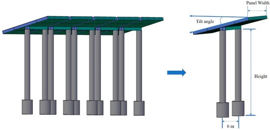
Figure 1.
A schematic diagram of the agricultural-electric symbiotic photovoltaic system.
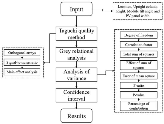
Figure 2.
A schematic flowchart of the conducted optimization method.
2.1. Taguchi Quality Method
The Taguchi quality method [47] is characterized by the use of orthogonal arrays to plan experiments and S/N ratios for analyzing the experiment data. Using an orthogonal array to design experiments allows the designer to study the influence of multiple controllable factors on the average and variance of a quality characteristic rapidly and economically. Using S/N ratios to analyze experiment data enables the product or process designer to easily find the optimum parameter combination. As the Taguchi method [48] can determine quality-influencing factors by identifying the experimental parameter values that best improve the data of the quality under consideration, thus finding the optimum parameter combination, it is used for the design parameters of the electrofarming symbiotic PV system in this study to solve the design parameter optimization problem and consequently enhance the quality and efficiency of the system.
- Orthogonal arrays
The orthogonal table is the most important tool of the Taguchi method. It allows changes to the control factors very effectively and systematically. Using the orthogonal array means fewer experiments are needed to obtain useful statistical information and reliable factorial effects. It is different from the full factorial experiment design (involving too many experiments) and fractional factorial experiment design (requiring too complicated an experimental method). The orthogonal array used in this study was L9(34), meaning there are nine experiments and four three-level factors.
- 2.
- Signal-to-noise ratio
In Taguchi experiment design, in order to measure experimental effectiveness, a function of the design factor is sometimes used as the standard, in a process known as effectiveness evaluation. The Taguchi experimental design method designates a statistical parameter for this effectiveness evaluation based on quality loss, called the signal to noise (S/N) ratio. The PV electrofarming symbiotic system of this study is aimed at high power generation and adequate hours of sunshine on crops, so the two quality characteristics were Larger-the-Better characteristics, and the S/N ratio is:
where MSD (mean squared deviation) is the average of deviation squared; yi is the measured value of quality i; and n is the total number of measurements.
S/N ratio = −10 log MSD
- 3.
- Main effect analysis
Based on the experimental plan derived from the orthogonal array and performing the experiment according to the plan, the experimental data for the various parameter combinations in the orthogonal array can be obtained, and the response table established. First of all, a quality indicator (i.e., the S/N ratio) is calculated from the experimental data values, the calculation approach depending on the nature of the quality characteristic. The average response value for the various factor levels is calculated, and then the main effect value of the various factor levels is computed with the data being rendered into a response table to allow analysis of the effect of the factors. The larger the main effect value of a factor is, the greater the influence that factor has on the system, in comparison with the other factors. On the other hand, if the main effect value of a factor is much smaller than that of the other factors, its effect on improving quality is insignificant.
where n is the number of level categories of the factor; m is the number of level i observations in the factor column of the orthogonal array; and yi is the S/N ratio of each i level row.
2.2. Grey Relational Analysis
Design parameter analysis of the PV electrofarming symbiotic system requires an appropriate mathematical model to be built to study the relationship of the two quality characteristics, power generation, and crop sunshine time resulting from the orthogonal array experiment seeking target values. The first step is to analyze the differences in the quality characteristics of the electrofarming system resulting from the different design parameter choices, and to understand the relationship with target values.
This paper adopted the Grey Relational Analysis proposed by Grey theory [49] to determine the relationship of the power generation and sunshine time results from the various orthogonal array experiments to the target values.
Grey Relational Analysis of the power-generation sunshine time symbiotic system is defined as follows:
- Target values of power generation and sunshine time of the PV electrofarming symbiotic system:
Reference sequence:
- 2.
- Power generation and sunshine time results from the various orthogonal array experiments of the symbiotic PV electrofarming system:
Xi = (x1(1), x1(2)), i = 1, 2, …, 9
- 3.
- The relationship between target values and experimental observations is expressed by the correlation coefficient:
Indicating the point relation of Xi to X0 at point k.
The characterizes the degree to which and are related, at point k, representing local characteristics of the relation between , . The mean of is known as the grey relational grade of to .
The calculation procedure of grey relational grade [50] is as follows:
Step 1: Calculate the initial value term (or mean term) of the various sequences
Step 2: Calculate the difference sequence
Step 3: Calculate the two-stage maximum difference and minimum difference
Step 4: Calculate the correlation coefficient
Step 5: Calculate the grey relational grade
After the target values for power generation and sunshine time of the electrofarming system are inputted as a reference sequence, the relational grade of the observations resulting from the L9 orthogonal array experiments can be worked out. When main effect analysis is performed, the optimal PV electrofarming design parameter combination can be derived from the response graph and response table.
2.3. Analysis of Variance
After an experiment designed according to the Taguchi method, the experimental data are processed by ANOVA to obtain comprehensive experimental results. The application of ANOVA has two purposes: one is to evaluate experimental error, the other one is to test the importance of the factors. An ANOVA performed on experimental data can separate the influence of the various control factors on experimental error, free from subjective evaluation. The importance of the factors is displayed as quantized values, not omitting important factors, through which it increases the accuracy of prediction.
The equations for computing and the methods of ANOVA are:
- Degree of freedom (DOF):
The DOF of a single factor equals its level number minus one; the total DOF is the total number of experiments minus one, the error DOF (DOFE) is the total DOF minus the sum of the DOFs of the various factors. The DOFs of the four factors of this study are all 2.
- 2.
- Correction factor
- 3.
- Total sum of squares:
- 4.
- Main effect sum of squares (SS):
The SS is the variation of the various factors. If factor p has n levels and each level has m observed values, the sum of squares of factor p is expressed as:
where Ai is the value of the experimental observations for level i.
- 5.
- Error sum of squares:
- 6.
- Mean square and error mean of square:
- 7.
- F-ratio:
The F-ratio represents the relationship between factorial effect and error variance. A larger F-ratio represents a more significant effect of the factor on the system, so the F-ratio can be used to arrange the factors in order of importance. If the F-ratio is smaller than 1, the factorial effect is slight. If the F-ratio is larger than 2, the factorial effect is strong. If the F-ratio is larger than 4, the factor has quite great effect. The F-ratio is defined as the mean square of the factor divided by the mean square of pooled error.
- 8.
- p-value:
The smaller the p-value, the more important the influence of the factor on the system.
- 9.
- Percent of contribution
The percent of contribution is the proportion of each factor in the main effect of the sum of squares, which represents the proportion of each factor’s effect on the quality.
2.4. Confidence Interval
The ANOVA importance and contribution analyses have evaluation procedures applicable to the control factors selected by the PV electrofarming symbiosis design. The factor combinations that best improve the experimental results can be predicted from the response table and response graph. A confirmation experiment is performed to determine whether the experimental results and prediction results line up with a probability in a certain confidence interval or not, so as to confirm whether the mathematical model built for the data from the orthogonal array experiments is appropriate. The S/N ratio in the optimum condition (SN) can be predicted with an additive model using the obtained optimum factor level setting value. The equation used to compute SN is:
where is the general average of the S/N ratio; and Fi is the S/N ratio of significant factor level value i.
In order to effectively evaluate the observed values, the confidence interval must be calculated. The equation used to compute CI is expressed as follows:
where is the F value with significance level α; α is the significance level, the confidence level is 1-α; is the DOF of pooled error mean square; MSE is the pooled error mean square; and neff is the effective observed value.
Finally, the 95% confidence interval is used to validate whether the predicted average is effective or not. The verification expression is:
3. Results and Discussions
First, the question of what control factors and level values would exert an influence on quality characteristics was considered. Based on prior research experience and discussion with senior engineers at PV equipment manufacturers, efforts were made to choose appropriate factors and levels. The PVsyst 7.2.0 software package was employed for annual PV power generation simulation analysis and the SunHours SketchUp plugin was used for annual hours of sunshine simulation analysis, providing a range of possible parameters which could be chosen. The cumulative hours of sunshine on farm land was divided by annual hours of sunshine to obtain a percentage figure for hours of sunshine on farm land.
Level values which could induce qualitative variability in power generation and sunshine time were determined, so as to provide an appropriate scope for design. Finally, from PV design parameters, the four control factors of location, height, angle of panel, and PV width were selected from the available parameters provided by PVsyst and SunHours for the experiment; and PV power generation and hours of sunshine on farm land were set as quality characteristics. The targeted figures for PV power generation and hours of sunshine on farm land, in the locations shown in Table 1, were non-specifically as large as possible. Thus, the Larger-the-Better characteristic type was selected for them, and S/N ratios were calculated as in Equation (1). The control factors and levels for the experiment are also shown in Table 1. From Table 1, the control factors and their level values were incorporated into an L9(34) orthogonal array as the experimental schedule. A total of nine experiments were performed following the experimental design, and the S/N ratio of each experiment was calculated from the experiment data. The results are shown in Table 2.

Table 1.
Control factor level value planning table.
Table 2.
L9 Orthogonal table and experimental results.
3.1. Taguchi Method: Single Quality Optimality Analysis
Quality Characteristic 1: PV Power Generation
In the response table (Table 3) and response graph (Figure 3), the larger the difference value, the greater the influence of that control factor on PV power generation. Table 3 shows the significance level of influence of location on PV power generation is 0.8560, that of the module tilt angle is 0.2430, that of the upright column height is 0.0067, and that of the PV panel width is 0.0066. Therefore, the order of the factors in terms of their significance is location > module tilt angle > upright column height > PV panel width.
Table 3.
The response table of PV power generation.
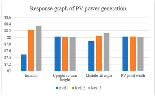
Figure 3.
Response graph of PV power generation.
In addition, the analysis of variance table calculated from the S/N ratios of Table 2 is shown in Table 4. It can be seen from the table that for PV power generation, the influence of control factors B and D is relatively small, so they are listed as pooled error. On the other hand, the F ratios of control factors A and C are both greater than 4, the p-values are both very small, and the confidence interval is greater than 95%, which means that the effects of these factors are quite large. These factors are significant factors. For PV power generation, the significant factors are A (Location) and C (Tilt). In terms of the degree of contribution, factor A is responsible for 87.42% of the influence, and factor C is 12.52% of the influence.
Table 4.
The ANOVA table of PV power generation.
The optimization parameter design condition is A3B1C3D1 according to the response table (Table 2) and the response graph (Figure 3), indicating a location in Tainan, an upright column height of 4 m, a module tilt angle of 15°, and a PV panel width of 1 m.
Quality Characteristic 2: Sunhours on Farm Land
In Table 5 and Figure 4, the larger the difference value, the greater the influence of that control factor on sunhours on farm land. Table 5 shows the significance level of influence of PV panel width on sunhours on farm land is 0.5616, that of the upright column height is 0.4119, that of the module tilt angle is 0.0625, and that of the location is 0.0115. Therefore, the order of the factors in terms of their significance is PV panel width > upright column height > module tilt angle > location.
Table 5.
Response table of sunhours on farm land.
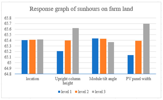
Figure 4.
Response graph of sunhours on farm land.
Additionally, according to the ANOVA of S/N ratios in Table 2, as shown in Table 6, for sunhours on farm land, the control factors A and C have only a very slight influence, so they are listed as pooled error. On the other hand, the F ratios of control factors B and D are larger than 4, the p-values are both very small, and the confidence interval is greater than 95%, meaning the factors have considerable effect. So those factors are significant factors. For sunhours on farm land, the significant factors are B (module height) and D (panel width). In terms of the degree of contribution, factor B is responsible for 20.74% of the influence, and factor D 78.13% of the influence.
Table 6.
The ANOVA table of sunhours on farm land.
The optimized parameter design condition is A3B3C1D3 according to the response table (Table 6) and the response graph (Figure 5), indicating a location in Tainan, an upright column height of 6 m, a module tilt angle of 5°, and a PV panel width of 3 m.
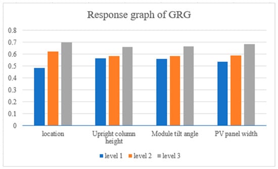
Figure 5.
The response graph of GRG.
3.2. Grey Relational Analysis: Multi-Quality Optimization Analysis
For different single quality characteristics, the obtained orders of significant factors and optimized parameter design conditions may be inconsistent, as seen in Table 4 and Table 6.
Therefore, to consider the optimization of parameter design conditions for two quality characteristics simultaneously, the results of PV power generation and sunhours on farm land must be quantized into a single index before analysis.
The grey correlation coefficient of Grey Relational Analysis can represent the deviation of experiment data from a reference point. In order to understand the influence of experiment data, the reference sequence was set as the optimal values of the experiments of the L9 orthogonal array, and the comparison sequence was the values to be compared. The grey correlation grade represents the deviation from this optimum design of the symbiotic electrofarming PV system. The value can be calculated by a weighting of the grey correlation coefficients. Using Grey Relational Analysis for analyzing the optimum multi-quality design parameter combination, the study adopted the maximum S/N values of PV power generation and sunhours on farm land from the L9 orthogonal array experiments as reference sequence, i.e., X0 = (88.464, 65.865). The difference sequence, grey correlation coefficient and correlation grade calculation results of the reference sequence and the sequences of the orthogonal array experiments are shown in Table 7. The results for grey relational grade (GRG) are collated with the factors of the L9 orthogonal array experiments in Table 8.
Table 7.
Difference sequences, grey correlation coefficients, and relational grades of L9 orthogonal array experiments.
Table 8.
Grey Relational Analysis results of L9 orthogonal array experiment.
Table 8 shows the GRG for the various experiments, which can be interpreted as the influence of individual experiments on the overall experiment. The larger the value is, the closer to the ideal experiment. As there are four factors in this study and each factor has three levels, the single-factor experiment (full factorial experiment) would have 81 sets of results. This study employed the L9 orthogonal array to efficiently perform nine experiments, but the remaining 72 might have produced better results for single quality optimization, especially considering the quality characteristics were PV power generation and sunhours on farm land. Thus, GRG averaged over different observation should be used for analyzing and calculating the results. The average GRG is like an S/N ratio, and its purpose is to determine the response relation between the factors and experiment. The average GRG of the different levels of the different design parameters is shown in the response table (Table 9) and response graph (Figure 5) and are obtained by main effect analysis.
Table 9.
The response table of GRG.
Table 9 and Figure 5 show the parameters with the greatest influence on the quality of the symbiotic electrofarming PV system. The larger the difference value is, the greater is the influence of the control factor on PV power generation and sunhours on farm land. It is observed that the upright column height and module tilt angle have the minimum influence on the quality characteristics. The difference values are 0.0981 and 0.1021, respectively. Location and PV panel width have relatively significant influence on design parameters. The difference values are 0.2155 and 0.1481, respectively, with location the most influential design parameter. Therefore, the order of the factors in terms of their significance is location > PV panel width > module tilt angle > upright column height. In addition, the optimal parameter design condition is A3, B3, C3, and D3, indicating a location in Tainan, an upright column height of 6 m, a module tilt angle of 15°, and a PV panel width of 3 m. If there are differences between the optimum parameters produced by Grey Relational Analysis and those derived from the Taguchi method, the reason is that the Taguchi method only analyzes one quality characteristic at a time. If there are multiple characteristics, Grey Relational Analysis must be used.
A confirmation experiment on the results of single-quality and multi-quality optimization was carried out. First of all, theoretically predicted values were calculated from those factors which were significant in the ANOVA table. Using Equation (20), the predicted values of PV power generation and sunhours on farm land were 26,507 and 1979, respectively. The 95% confidence intervals were 26,384–26,630 kWh and 1944–2014 h. In Table 10, for the single-quality optimizations, only one quality characteristic falls inside the 95% confidence interval. For example, for the PV power generation quality characteristic, PV power generation of the confirmation experiment falls inside the 95% confidence interval, but sunhours on farm land lies outside. For the sunhours on farm land quality characteristic, the situation is reversed. PV power generation of the confirmation experiment lies outside the 95% confidence interval, but sunhours on farm land falls within the 95% confidence interval.
Table 10.
Confirmation experiment results of single-quality optimization and multi-quality optimization.
However, for the multi-quality optimization, PV power generation and sunhours on farm land both lie inside the 95% confidence interval, meaning influences on both quality characteristics receive full expression in this symbiotic electrofarming PV system study. The electrofarming symbiosis PV system built on the basis of the multi-quality optimization condition arrived at in the study is shown in Figure 6 and Figure 7.
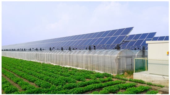
Figure 6.
View of optimized symbiotic electrofarming system (1).
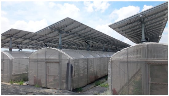
Figure 7.
View of optimized symbiotic electrofarming system (2).
Finally, the benefits of the symbiotic electrofarming PV system built in this study were assessed. The basis of evaluation of the symbiotic electrofarming PV system of this study is described in Table 11.
Table 11.
Specification of the symbiotic electrofarming PV system.
While the total installed capacity per unit system of this study is 63.825 Wp/m2, the total installed capacity per unit system of an international comparison is 45 Wp/m2 [51], which is 41.8% lower. Therefore, the symbiotic electrofarming PV system of this study not only allows crops to grow in adequate amounts of sunshine, but also increases the power benefits by 41.8%.
This study provides higher IRR along with good productive vegetables. There are a bunch of vegetables that grow in shade, such as tomato, potato, broccoli, etc. Table 12 shows the comparative study of different electrofarming PV systems in different places. Poonia et al. [52] studied the electrofarming PV system where farm plot size was 4624 m2 in India. The total power generation capacity was 520 kW. In India, sunshine is available throughout the year with more sunshine hours than studies [53,54] shown in Table 12. In India, it is assumed a 12% bank interest in order to build the PV system and their IRR was 20.38% [52]. Moreda et al. [53] built the electrofarming PV system in Spain where a good amount of sunshine is not available all the time. Their power generation capacity is high but IRR is low due to the lack of availability of the sunshine. Damnoen et al. [54] experimented the electrofarming PV system in Thailand. The power generation capacity is 100,000 kW and their IRR was 15.62%. The electrofarming PV system is so large that it would not be acceptable for farmers. In order to build a system which can provide both electricity and agricultural production, it needs to be acceptable by farmers so that most of the farmers benefit from this electrofarming system. The above studies [52,53,54] considered building the electrofarming PV system in their respective places in order to get the maximum IRR. However, they do not study the optimization of the land, PV cells, and PV location, etc. Our study focuses not only on obtaining IRR, but how to get the best production in vegetables and high-power generation. This study uses a farm plot size of 400 m2 and the total power generation capacity is 25.53 kW, which can be affordable by farmers and will be benefited by this electrofarming PV system.
Table 12.
Comparative study of the electrofarming PV system.
With the results of multi-quality optimization now obtained, the results of single-quality optimization and multi-quality optimization can be analyzed together. It is obvious that single-quality optimization produces significant differences in factor significance. For PV power generation, location was most significant, but PV panel width was least significant. For sunhours on farm land, on the other hand, the situation was the reverse. PV panel width was most significant, whereas location was least significant. However, according to the multi-quality optimization results, location was the most significant, and PV panel width was second most significant. In other words, GRA considered the significance of location and PV panel width simultaneously. The result showed that PV power generation and sunhours on farm land both lie inside the 95% confidence interval which provides optimized result of the particular location. The study also showed the cultivation of vegetables underneath the PV panel. The overall IRR is about 10.88%, which is promising and feasible in the region being situated above the tropic cancer where sunlight is not directly overhead. The combined systems of PV and agriculture could offer a win-win situation across many sectors, increases crop production, water efficient, and efficiency of PV arrays. By adopting symbiotic system can help to build resilient food-production and energy-generation systems [55].
4. Conclusions
This study combined Grey Relational Analysis with the Taguchi method to determine the optimum combination of symbiotic electrofarming PV design parameters with a minimal number of experiments. The Grey Relational Analysis response table and response graph showing the design parameter combinations of the symbiotic electrofarming PV system in Taiwan reveal the best set is a Tainan location, an upright column height of 6 m, a module tilt angle of 15°, and a PV panel width of 3 m. The relatively significant factors that influenced the single quality PV power generation were the location and module tilt angle, and relatively significant factors which influenced the single quality sunhours on farm land were the other two, PV panel width and upright column height. However, the relatively significant factors which influenced the two quality characteristics simultaneously were location and PV panel width. The parameter combination of multi-quality optimization was validated by a confirmation experiment. The confirmation experiment values of PV power generation and sunhours on farm land fell within the 95% confidence interval, which shows the reliability of the experimental results, indicates the selection of experimental factors to be appropriate, and is evidence supporting the viability of the methods of this experiment. According to a benefit comparison and validation analysis, the total installed capacity per unit system of this study was 63.825 Wp/m2, which was 41.8% higher than the total installed capacity per unit system of an international comparison. Therefore, the symbiotic electrofarming PV system designed by these methods not only allowed crops to grow in adequate amounts of sunshine, but also increased the power benefits by 41.8%. In other words, the multi-quality optimization method proposed in this study enables a carefully-crafted symbiotic electrofarming PV system to satisfy the needs of both energy and agricultural production. It can help to implement policy based on the sustainable development to a nation.
The limitation of the study depends on location, column height, and availability of sunhours. The performance may vary depending on the location, environment conditions, and sunhours available to that particular region, otherwise this study has the suitable application in order to get the optimal parameters. The height of the column must be maintained at least 2 m above the ground to allow the efficient use of agricultural machinery. Determining the vegetable which grows under low light. The future study can be focus on vegetables growing underneath the PV system, including more factor such as environment conditions for determining the optimal parameters.
Author Contributions
Methodology, conceptualization, Supervision, and verification: C.-F.J.K.; writing—original draft, methodology, and Software: T.-L.S.; investigation, and formal analysis: C.-Y.H.; conceptualization and data curation: H.-C.L.; writing—review and editing, resources, and visualization: J.B.; methodology, editing, review: I.K. All authors have read and agreed to the published version of the manuscript.
Funding
The research was supported by the Ministry of Science and Technology of the Republic of China under the grant No: MOST 110-2622-E-011 -012-.
Institutional Review Board Statement
Not applicable.
Informed Consent Statement
Not applicable.
Data Availability Statement
Not applicable.
Acknowledgments
The financial support provided by Bureau of Energy, Ministry of Economic Affairs, Taiwan, R.O.C. (Contract No: 112-S0102) is gratefully acknowledged.
Conflicts of Interest
The authors declare no conflict of interest.
References
- Elahi, E.; Khalid, Z. Estimating smart energy inputs packages using hybrid optimisation technique to mitigate environmental emissions of commercial fish farms. Appl. Energy 2022, 326, 119602. [Google Scholar] [CrossRef]
- Elahi, E.; Khalid, Z.; Tauni, M.Z.; Zhang, H.; Lirong, X. Extreme weather events risk to crop-production and the adaptation of innovative management strategies to mitigate the risk: A retrospective survey of rural Punjab, Pakistan. Technovation 2022, 117, 102255. [Google Scholar] [CrossRef]
- Abbas, A.; Waseem, M.; Ahmad, R.; Khan, K.A.; Zhao, C.; Zhu, J. Sensitivity analysis of greenhouse gas emissions at farm level: Case study of grain and cash crops. Environ. Sci. Pollut. Res. 2022, 29, 82559–82573. [Google Scholar] [CrossRef] [PubMed]
- Abbas, A.; Zhao, C.; Waseem, M.; Ahmad, R. Analysis of energy input–output of farms and assessment of greenhouse gas emissions: A case study of cotton growers. Front. Environ. Sci. 2022, 9, 826838. [Google Scholar] [CrossRef]
- Droege, P. Renewable energy and the city: Urban life in an age of fossil fuel depletion and climate change. Bull. Sci. Technol. Soc. 2002, 22, 87–99. [Google Scholar] [CrossRef]
- Moss, R.H.; Edmonds, J.A.; Hibbard, K.A.; Manning, M.R.; Rose, S.K.; Van Vuuren, D.P.; Carter, T.R.; Emori, S.; Kainuma, M.; Kram, T.; et al. The next generation of scenarios for climate change research and assessment. Nature 2010, 463, 747–756. [Google Scholar] [CrossRef] [PubMed]
- Wiginton, L.K.; Nguyen, H.T.; Pearce, J.M. Quantifying rooftop solar photovoltaic potential for regional renewable energy policy. Comput. Environ. Urban Syst. 2010, 34, 345–357. [Google Scholar] [CrossRef]
- de Wild-Scholten, M.J.; Alsema, E.A.; Ter Horst, E.W.; Bächler, M.; Fthenakis, V.M. A cost and environmental impact comparison of grid-connected rooftop and ground-based PV systems. In Proceedings of the 21th European Photovoltaic Solar Energy Conference, Dresden, Germany, 4–8 September 2006. [Google Scholar]
- Nonhebel, S. Renewable energy and food supply: Will there be enough land? Renew. Sustain. Energy Rev. 2005, 9, 191–201. [Google Scholar] [CrossRef]
- Calvert, K.; Mabee, W. More solar farms or more bioenergy crops? Mapping and assessing potential land-use conflicts among renewable energy technologies in eastern Ontario, Canada. Appl. Geogr. 2015, 56, 209–221. [Google Scholar] [CrossRef]
- Trommsdorff, M.; Kang, J.; Reise, C.; Schindele, S.; Bopp, G.; Ehmann, A.; Weselek, A.; Högy, P.; Obergfell, T. Combining food and energy production: Design of an agrivoltaic system applied in arable and vegetable farming in Germany. Renew. Sustain. Energy Rev. 2021, 140, 110694. [Google Scholar] [CrossRef]
- Dinesh, H.; Pearce, J.M. The potential of agrivoltaic systems. Renew. Sustain. Energy Rev. 2016, 54, 299–308. [Google Scholar] [CrossRef]
- Hsu, H.M.; Cheng, A.; Chao, S.J.; Chang, J.R.; Teng, L.W.; Chen, S.C. The Grey Relational Analysis of Quality Investigation of Concrete Containing Solar PV Cells. MATEC Web Conf. 2015, 27, 01006. [Google Scholar] [CrossRef]
- Tiwari, G.N.; Mishra, R.K.; Solanki, S.C. Photovoltaic modules and their applications: A review on thermal modelling. Appl. Energy 2011, 88, 2287–2304. [Google Scholar] [CrossRef]
- Almodfer, R.; Zayed, M.E.; Abd Elaziz, M.; Aboelmaaref, M.M.; Mudhsh, M.; Elsheikh, A.H. Modeling of a solar-powered thermoelectric air-conditioning system using a random vector functional link network integrated with jellyfish search algorithm. Case Stud. Therm. Eng. 2022, 31, 101797. [Google Scholar] [CrossRef]
- El-Hadary, M.I.; Senthilraja, S.; Zayed, M.E. A Hybrid System Coupling Spiral Type Solar Photovoltaic Thermal Collector and Electrocatalytic Hydrogen Production Cell: Experimental Investigation and Numerical Modeling. Process. Saf. Environ. Prot. 2023, 170, 1101–1120. [Google Scholar] [CrossRef]
- Bae, S.; Nam, Y. Feasibility analysis for an integrated system using photovoltaic-thermal and ground source heat pump based on real-scale experiment. Renew. Energy 2022, 185, 1152–1166. [Google Scholar] [CrossRef]
- Zayed, M.E.; Zhao, J.; Elsheikh, A.H.; Li, W.; Sadek, S.; Aboelmaaref, M.M. A comprehensive review on Dish/Stirling concentrated solar power systems: Design, optical and geometrical analyses, thermal performance assessment, and applications. J. Clean. Prod. 2021, 283, 124664. [Google Scholar] [CrossRef]
- Agostini, A.; Colauzzi, M.; Amaducci, S. Innovative agrivoltaic systems to produce sustainable energy: An economic and environmental assessment. Appl. Energy 2021, 281, 116102. [Google Scholar] [CrossRef]
- Valle, B.; Simonneau, T.; Sourd, F.; Pechier, P.; Hamard, P.; Frisson, T.; Ryckewaert, M.; Christophe, A. Increasing the total productivity of a land by combining mobile photovoltaic panels and food crops. Appl. Energy 2017, 206, 1495–1507. [Google Scholar] [CrossRef]
- Qoaider, L.; Steinbrecht, D. Photovoltaic systems: A cost competitive option to supply energy to off-grid agricultural communities in arid regions. Appl. Energy 2010, 87, 427–435. [Google Scholar] [CrossRef]
- Cossu, M.; Murgia, L.; Ledda, L.; Deligios, P.A.; Sirigu, A.; Chessa, F.; Pazzona, A. Solar radiation distribution inside a greenhouse with south-oriented photovoltaic roofs and effects on crop productivity. Appl. Energy 2014, 133, 89–100. [Google Scholar] [CrossRef]
- Gao, Y.; Dong, J.; Isabella, O.; Santbergen, R.; Tan, H.; Zeman, M.; Zhang, G. Modeling and analyses of energy performances of photovoltaic greenhouses with sun-tracking functionality. Appl. Energy 2019, 233, 424–442. [Google Scholar] [CrossRef]
- Li, C.; Wang, H.; Miao, H.; Ye, B. The economic and social performance of integrated photovoltaic and agricultural greenhouses systems: Case study in China. Appl. Energy 2017, 190, 204–212. [Google Scholar] [CrossRef]
- Marrou, H.; Wéry, J.; Dufour, L.; Dupraz, C. Productivity and radiation use efficiency of lettuces grown in the partial shade of photovoltaic panels. Eur. J. Agron. 2013, 44, 54–66. [Google Scholar] [CrossRef]
- Santra, P.; Singh, R.K.; Meena, H.M.; Kumawat, R.N.; Mishra, D.; Jain, D.; Yadav, O.P. Agri-voltaic system: Crop production and photovoltaic-based electricity generation from a single land unit. Indian Farming 2018, 68, 20–23. [Google Scholar]
- Weselek, A.; Ehmann, A.; Zikeli, S.; Lewandowski, I.; Schindele, S.; Högy, P. Agrophotovoltaic systems: Applications, challenges, and opportunities. A review. Agron. Sustain. Dev. 2019, 39, 35. [Google Scholar] [CrossRef]
- Van Campen, B.; Guidi, D.; Best, G. Solar Photovoltaics for Sustainable Agriculture and Rural Development; InRural Development, Fao Publication: Rome, Italy, 2000. [Google Scholar]
- Artru, S.; Lassois, L.; Vancutsem, F.; Reubens, B.; Garré, S. Sugar beet development under dynamic shade environments in temperate conditions. Eur. J. Agron. 2018, 97, 38–47. [Google Scholar] [CrossRef]
- Castellano, S. Photovoltaic greenhouses: Evaluation of shading effect and its influence on agricultural performances. J. Agric. Eng. 2014, 45, 168–175. [Google Scholar] [CrossRef]
- Beck, M.; Bopp, G.; Goetzberger, A.; Obergfell, T.; Reise, C.; Schindele, S. Combining PV and food crops to Agrophotovoltaic–optimization of orientation and harvest. In Proceedings of the 27th European Photovoltaic Solar Energy Conference and Exhibition, EU PVSEC, Frankfurt, Germany, 24–28 September 2012. [Google Scholar]
- Park, S.; Chuang, H.S.; Kwon, J.S. Numerical study and Taguchi optimization of fluid mixing by a microheater-modulated alternating current electrothermal flow in a Y-shape microchannel. Sens. Actuators B Chem. 2021, 329, 129242. [Google Scholar] [CrossRef]
- Dutta, S.; Narala, S.K. Optimizing turning parameters in the machining of AM alloy using Taguchi methodology. Measurement 2021, 169, 108340. [Google Scholar] [CrossRef]
- Khalilarya, S.; Chitsaz, A.; Mojaver, P. Optimization of a combined heat and power system based gasification of municipal solid waste of Urmia University student dormitories via ANOVA and taguchi approaches. Int. J. Hydrogen Energy 2021, 46, 1815–1827. [Google Scholar] [CrossRef]
- Hernandez, B.A.; Gill, H.S.; Gheduzzi, S. Material property calibration is more important than element size and number of different materials on the finite element modelling of vertebral bodies: A Taguchi study. Med. Eng. Phys. 2020, 84, 68–74. [Google Scholar] [CrossRef] [PubMed]
- Kolasangiani, R.; Mohandes, Y.; Tahani, M. Bone fracture healing under external fixator: Investigating impacts of several design parameters using Taguchi and ANOVA. Biocybern. Biomed. Eng. 2020, 40, 1525–1534. [Google Scholar] [CrossRef]
- Lin, W.; Ma, Z.; Cooper, P.; Sohel, M.I.; Yang, L. Thermal performance investigation and optimization of buildings with integrated phase change materials and solar photovoltaic thermal collectors. Energy Build. 2016, 116, 562–573. [Google Scholar] [CrossRef]
- Zhang, F.; Wang, M.; Yang, M. Successful application of the Taguchi method to simulated soil erosion experiments at the slope scale under various conditions. Catena 2021, 196, 104835. [Google Scholar] [CrossRef]
- Kuo, C.F.; Dong, M.Y.; Yang, C.P. Optimization of the water-based polyurethane with acrylate terminal process in nylon fabrics application using the Taguchi-based gray relational analysis method. Text. Res. J. 2021, 91, 1197–1210. [Google Scholar] [CrossRef]
- Kazemian, A.; Parcheforosh, A.; Salari, A.; Ma, T. Optimization of a novel photovoltaic thermal module in series with a solar collector using Taguchi based grey relational analysis. Sol. Energy 2021, 215, 492–507. [Google Scholar] [CrossRef]
- Senthilkumar, S.; Karthick, A.; Madavan, R.; Moshi, A.A.; Bharathi, S.S.; Saroja, S.; Dhanalakshmi, C.S. Optimization of transformer oil blended with natural ester oils using Taguchi-based grey relational analysis. Fuel 2021, 288, 119629. [Google Scholar] [CrossRef]
- Suji, D.; Adesina, A.; Mirdula, R. Optimization of self-compacting composite composition using Taguchi-Grey relational analysis. Materialia 2021, 15, 101027. [Google Scholar] [CrossRef]
- Kuo, C.F.; Su, T.L.; Jhang, P.R.; Huang, C.Y.; Chiu, C.H. Using the Taguchi method and grey relational analysis to optimize the flat-plate collector process with multiple quality characteristics in solar energy collector manufacturing. Energy 2011, 36, 3554–3562. [Google Scholar]
- Canbolat, A.S.; Bademlioglu, A.H.; Arslanoglu, N.; Kaynakli, O. Performance optimization of absorption refrigeration systems using Taguchi, ANOVA and Grey Relational Analysis methods. J. Clean. Prod. 2019, 229, 874–885. [Google Scholar] [CrossRef]
- Üstüntağ, S.; Şenyiğit, E.; Mezarcıöz, S.; Türksoy, H.G. Optimization of coating process conditions for denim fabrics by Taguchi method and Grey relational analysis. J. Nat. Fibers 2020, 19, 685–699. [Google Scholar] [CrossRef]
- Pascaris, A.S.; Schelly, C.; Pearce, J.M. A first investigation of agriculture sector perspectives on the opportunities and barriers for agrivoltaics. Agronomy 2020, 10, 1885. [Google Scholar] [CrossRef]
- Karna, S.K.; Sahai, R. An overview on Taguchi method. Int. J. Eng. Math. Sci. 2012, 1, 1–7. [Google Scholar]
- Ross, P.J. Taguchi Techniques for Quality Engineering: Loss Function, Orthogonal Experiments, Parameter and Tolerance Design, 2nd ed.; McGraw-Hill: New York, NY, USA, 1996. [Google Scholar]
- Julong, D. Introduction to grey system theory. J. Grey Syst. 1989, 1, 1–24. [Google Scholar]
- Kuo, C.F.; Su, T.L. Gray relational analysis for recognizing fabric defects. Text. Res. J. 2003, 73, 461–465. [Google Scholar] [CrossRef]
- Agrivoltaics: Opportunities for Agriculture and the Energy Transition; Fraunhofer ISE: Freiburg im Breisgau, Germany, 2020.
- Poonia, S.; Jat, N.K.; Santra, P.; Singh, A.K.; Jain, D.; Meena, H.M. Techno-Economic Evaluation of Different Agri-Photovoltaic Designs for the Hot Arid Ecosystem of Western Rajasthan, India. SSRN 2021. [Google Scholar] [CrossRef]
- Moreda, G.P.; Muñoz-García, M.A.; Alonso-García, M.C.; Hernández-Callejo, L. Techno-Economic Viability of Agro-Photovoltaic Irrigated Arable Lands in the EU-Med Region: A Case-Study in Southwestern Spain. Agronomy 2021, 11, 593. [Google Scholar] [CrossRef]
- Damnoen, P.; Ketjoy, N. Analysis of investment models for megawatt scale photovoltaic power plant in Thailand. J. Renew. Energy Smart Grid Technol. 2019, 14. Available online: https://ph01.tci-thaijo.org/index.php/RAST/article/view/128130 (accessed on 8 March 2023).
- Benefits of Agrivoltaics across the Food-Energy-Water Nexus. Available online: https://www.nrel.gov/news/program/2019/benefits-of-agrivoltaics-across-the-food-energy-water-nexus.html (accessed on 3 March 2023).


Disclaimer/Publisher’s Note: The statements, opinions and data contained in all publications are solely those of the individual author(s) and contributor(s) and not of MDPI and/or the editor(s). MDPI and/or the editor(s) disclaim responsibility for any injury to people or property resulting from any ideas, methods, instructions or products referred to in the content. |
© 2023 by the authors. Licensee MDPI, Basel, Switzerland. This article is an open access article distributed under the terms and conditions of the Creative Commons Attribution (CC BY) license (https://creativecommons.org/licenses/by/4.0/).