Abstract
Water shortage and its interconnected and integrated management is one of the life crises in recent years. Factors such as population growth, plurality of population needs, traditional farming methods, climate change, and water waste are among the contributing factors to this crisis. The complexity of water sources and consumption systems makes the management and decision-making related to this resource very difficult. This research aims to study the effective factors in the water sources and consumption system of Rafsanjan city and suggests a simulated model of water shortage and its causes. In this research, water shortage crises were simulated using system dynamics. Important variables of the water shortage crisis are identified and optimized using the Design of Experiments (DOE) method. Vensim software was considered to illustrate the simulations of five scenarios aiming at better managing water resources and dealing with the water shortage crisis in this city.
1. Introduction
Water is known as the most vital natural resource, such that its severe shortage brings global concerns [1,2]. Its scarcity has the potential to seriously restrict the development and continuation of human activities [3]. Furthermore, water resources play a critical role in population, social, and economic development [4]. As such, efficient management and planning are essential for sustainable urban economic development [5]. Furthermore, many countries are experiencing challenges with water resources [3,6]. It is worth noting that the lack of fresh water has been known as a major crisis of the 21st century [7].
According to the United Nations Political Studies and Development Unit in 2010, 1.2 billion people (i.e., approximately one-fifth of the world’s population) live in areas suffering from a physical lack of water, while approximately 1.6 billion people live in areas suffering from economic water shortage. In addition, several plans indicate that 800 million people will live in countries or regions suffering from an absolute lack of water by 2025, such that two-thirds of the world’s population will encounter a severe shortage of water. Meanwhile, this report highlights that the Middle East and North Africa region will encounter a per capita reduction of annual renewable water resources from 750 m3 to 500 m3 by 2025 (Police Diplomate and Studies Branch, 2010).
In terms of water resources management, several investigations have been conducted. Guo et al. [8] developed an environmental system dynamics model titled Arhai system dynamics to support environmental management system planning in the Arhai Lake basin for sustainable local development. The proposed modeling was simulated, and a variety of decision actions and their dynamic consequences were investigated. Ho et al. [9] described a process to combine system dynamics. Parametric analysis effectively, systematically, and quantitatively assessed the strategies for water shortage solving. The economic advantages of local water resource planning and management were also revealed. In addition, they developed a system dynamics model called the Tianjin System Dynamics Model to integrate scientific management of Tianjin’s water resources. This model encompassed the information feedback managing the interactions within the system, which could combine level knowledge exceptions to simulate the behavior of the system at an integrated level. Accordingly, it provided logical predictive results to allocate and manage water resources. Kojiri et al. [3] investigated the severity of a water shortage in the future and its impact on the growth of human civilization using the world system dynamics model at the regional level. Six parts of activities were modeled in each continent to represent human society. Furthermore, some continental interactions (such as migration and trade) were considered to discuss the synergy of activities between different continents. The simulation results from 1960 to 2100 indicated that unlike other constraints (such as non-renewable resources and persistent pollution), water shortage would result in creating severe problems due to a persistent delay after its occurrence. Feng et al. [10] developed a water shortage risk assessment model using the risk assessment method based on information ambiguity theory in Yiwu City, China. In addition, they simulated water shortage risk changes based on the system dynamics model to confirm the theoretical results in addition to analyzing the carrying capacity of water resources in terms of an environmental approach. Dai et al. [11] developed a spatial system dynamics model to assess the water environment capacity in the Yongding River Basin in North China. Their study suggested the simultaneous consideration of economic growth and environmental preservation. Li [12] developed a model based on system dynamics for Suzhou water resources carrying capacity in China. Three different optimization programs for water resources were approved as follows: (1) continuation of the existing water usage; (2) water protection/storage; and (3) water exploitation. Wei et al. [13] developed a system dynamics model that takes into consideration the interactions between water resources and environmental, economic, and social flows. The social and economic effects of different levels of environmental flow allocation were surveyed in the Weihe River Basin of China. Xi and Poh [1] developed a system dynamics model called Singapore water, and then analyzed the long-term effects of various investment programs. They showed that investigating the underground water shortage and collecting surface water was not enough to achieve self-sufficiency in water. They employed system dynamics, artificial neural networks, and the Markov chain to model the water environmental system because of the limitations of traditional methods in surveys of the environmental carrying capacity of water and the complexity of its environmental system. The social components were modeled based on the Granger causality test using system dynamics. Sun et al. [4] categorized the effective macroeconomic factors in the optimal usage of water resources into five main sub-systems of economy, population, water supply and demand, water resources, pollution, and water management. They concluded that improving water supply rather than demand control was the main method to fill the gap between water supply and demand.
The literature review shows that the development of agriculture, the rapid growth of industries, the excessive expansion of the population, and other factors affect water demand every day. On the other hand, it requires proper planning to manage water resources and better exploit these valuable resources due to the limited amount of available water as well as the continuous increase in demand. More importantly, current and even future needs can be satisfied if the existing water resources are suitably exploited. Here, it is worth mentioning that optimal management and exploitation of water resources is the most effective step in preserving water resources and preventing possible water shortages. Hence, investigating the water status in different regions helps the proper exploitation of water resources such that the stability of water resources is provided by applying the best management scenario. Among the countries of the Middle East, Iran is currently facing serious water shortage problems. Droughts associated with excessive extraction of surface and underground water using a large network of hydraulic infrastructure as well as deep wells have aggravated the country’s water situation. The drying lakes, rivers, and wetlands, underground water reduction, land subsidence, degradation of water quality, soil erosion, desertification, and frequent dust storms have led to a water crisis in several countries [14]. On the other hand, desert life and arid and semi-arid areas are completely affected by underground water resources due to low rainfall; hence, the suitable management of underground water ensures sustainable development in those areas.
Recognition and exploration of a model for describing the water shortage crisis calls for a careful study of all system components as the water shortage is constantly changing. Static analyses do not produce an appropriate solution as they do not fully engage with time variations and the internal nature of the system. In contrast, the source of the model’s behavior is the system’s very nature. The system dynamics modeling technique is potent for understanding the system’s relationships and nature [15]. System dynamics has a more realistic look at the problem and can examine the effect of several causes on different dimensions. System dynamics go beyond the single-dimension and linear perspective and provide solutions to improve the status quo with a comprehensive look [16]. System dynamics focus on the system’s internal structure and can make relevant predictions using causal relationships between variables [17]. The real power of the system dynamics approach is designing the simulation model of the problem. Here, model means presentation and simplification of one part of the reality of the system dynamics. The system dynamics models enable the researcher to experience again, experiment with hypotheses, or change management policies. Quantitative computerized models are the most tangible aspect of system dynamics, developed from a complex system to examine the model’s behavior. The purpose of modeling is to develop a good understanding of the subject [18]. Currently, various software applications can be used to optimize the designed model, each of which has specific characteristics. For instance, Vensim is a powerful tool for simulation that provides the context for simulating, modeling, experimenting, and sensitivity analysis of dynamic complex systems by focusing on fundamental differential equations using pre-existing integrations. The software provides the context for modeling by identifying causal loops, finding leverage points, and using dynamic functions such as arrays, Monte Carlo sensitivity analysis, optimization, application interfaces, etc. [19]. System dynamics focuses on the way one quantity can affect others through the flow of physical entities and information. Often, such flows come back to the original quantity, causing a feedback loop. The behavior of the system is governed by these feedback loops. There are two important advantages of the system dynamics with Vensim software, which causes this approach to be used instead of other approaches. The interrelationship of different elements of the systems can be easily seen in terms of cause and effect. Thus, the true cause of the behavior can be identified. The other advantage is that it is possible to investigate which parameters or structures need to be changed to improve behavior.
Water resources management can definitely benefit from forward-looking decision-making using a comprehensive approach with system dynamics as a management tool. That is, hydrology and water resources management issues are complex, considering local weather conditions (such as changes in rainfall distribution patterns), groundwater surface water connections, natural reserves, human savings, population growth, and water demand. These features make system dynamics a suitable approach for hydrological and water resources management problems [20].
Thus, this research considers a system dynamics approach to provide some practical solutions for the water crisis problem in Rafsanjan. Some sub-objectives, such as identifying the effective and key effective factors of the water crisis, and simulating water resources, were considered. This paper attempts to answer the following questions:
- Which factors affect the water crisis in Rafsanjan?
- Which factors are sensitive and key?
- What are the optimal values of the factors affecting the water crisis?
- What scenarios can be defined for better management of water resources and related problems?
2. Research Methodology
This research developed a dynamic model for the water crisis in Rafsanjan city using a system dynamics model. The aim is to predict the water crisis over a hundred-year period. Variables of supply, agriculture, industry, and household (population) sub-systems were selected, and a dynamic system was utilized for simulation. By relying on dynamic feedback mechanisms in the system as well as causal loops, this paper demonstrates how events occurred, in which non-linear behaviors were expressed using storage and flow structures, time delays, and readbacks. The overall framework of the model is indicated in Figure 1. The data for this research were collected from different sources. The references for this data collection are specified in Table 1.
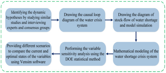
Figure 1.
The overall framework of the research model.

Table 1.
Data collection references.
In addition, the DOE statistical method, which was developed from the 1920s to 1930s at the Rothamsted Agricultural Experimental Station near London, England, was utilized to analyze the sensitivity of variables. This method was developed in four periods, namely, the agricultural period, the industrial period, the quality improvement period, and the period of using this method in the field of engineering sciences and various industries. This method can help better understand the working systems and their process procedures. Notably, observations of any system or process would lead to generating hypotheses and opinions about such, necessitating tests and rejection [21]. The modeling steps in the system dynamics are described as follows:
- i.
- The factors affecting water shortage and their relationship are hypothesized. A series of factors affecting water shortage are identified by studying similar studies and interviewing experts and consensus groups.
- ii.
- The causal loop diagram of the whole system is depicted using the dynamic hypotheses extracted from step i.
- iii.
- The stock-flow diagram is provided and the model is simulated. State-flow diagrams as a practical tool to show accumulations and flows within a model are presented. An abbreviation is considered for each variable to reveal equations showing the relationship of each variable.
- iv.
- Formulating the model and developing the mathematical model: this step shows the mathematical relationships used in the simulation of the dynamic model of the water shortage crisis system in Rafsanjan. Validation of system dynamics models should be performed to ensure the validity and usefulness of the model. The validation is a combination of activities starting from the beginning steps of modeling in the system dynamics approach. During these steps, investigating the model structure of a real system is considered based on the different dimensions and their agreement with each other, and whether the proposed model is suitable to accomplish the desired objective. On the other hand, testing the model and its validity increases the reliability of the model and raises confidence in its applicability. In this paper, experts’ opinions and multiple tests of the model by experts were used to assess the validity of the model.
- v.
- The sensitivity analysis of the variables is performed using DOE. DOE is a statistical method to obtain maximum information from a process by performing the minimum possible experiments. By DOE implementation, the optimal value of measurement results (i.e., solutions) or the conditions can be determined in which conflicting solutions are compatible. In this work, the importance of the key variables affecting the water shortage in Rafsanjan was identified by DOE. A comparison of the current and optimal status of the variables was then discussed, and solutions were provided to reach the optimal status of the variables.
- vi.
- Vensim software is considered to illustrate the simulations of five scenarios aimed at better managing the water resources and dealing with the water shortage crisis in this city.
3. Results and Discussions
The results obtained are described in this section using the following steps:
Step One: The causal loop diagram of the water crisis system was drawn in the first step of this research. Figure 2 illustrates the causal loop diagram of the whole system.
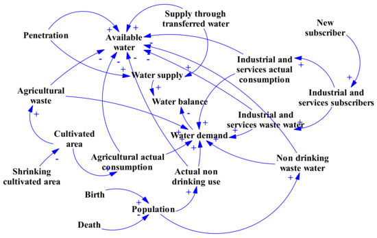
Figure 2.
Causal loop diagram of the water shortage crisis in Rafsanjan city.
This figure was provided using the dynamic hypotheses extracted from the literature study of relevant issues. The opinions and judgments of experts after holding semi-structured interviews with experts were also considered. Each arrow in the casual loop is marked with the (+) or (-), where (+) means that if the first variable is changed, the second variable will be changed in the same direction, whereas (-) indicates that if the first variable is changed the second variable will be changed in the opposite direction.
The available water amount variable should be mentioned as the variable that attracted the most attention. It can be predicted that by decreasing the amount of available water, a fundamental problem will arise, causing irreparable damage to the city, if not managed in proper time.
Step Two: Stock-flow diagram and model simulation were demonstrated.
The variables of the model along with their description and units are listed in Table 2, and the general state-flow diagram is depicted in Figure 3. In Table 2, an abbreviation was considered for each variable to write the formula and equation.
Table 2.
Description of stock-flow diagram variables.
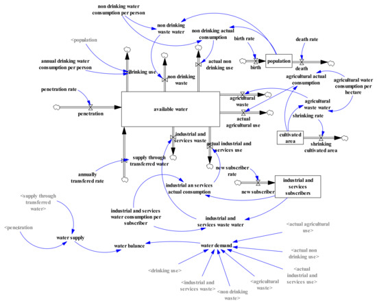
Figure 3.
Diagram of stock-flow of water shortage in Rafsanjan city.
Step Three: The model was formulated and the mathematical model was developed. The following equations represent the mathematical relationships used in the simulation of the dynamic model of the water shortage crisis system in Rafsanjan.
Equation (1) shows the total available water. The initial value of the stock variable of available water is equal to 4 billion m3. If the total available water is assumed as a large storage, then some amounts of water will enter this storage and some amounts of water will leave this storage.
The input variables of this storage are as follows:
- -
- The amount of water penetration to underground aquifers (Equation (2))
- -
- The amount of water transferred to the system (Equation (4))
The output variables of this storage are as follows:
- -
- The amount of water consumption in agriculture (Equation (20))
- -
- The amount of water waste in the agricultural sector (Equation (18))
- -
- The amount of drinking water consumed each year (Equation (6))
- -
- The amount of water used for non-potable water consumption (Equation (10))
- -
- The amount of non-potable water waste (Equation (8))
- -
- The amount of water consumption in industry and services (Equation (26))
- -
- The amount of water waste in industry and services (Equation (28))
AW = INTEG(P + STW − AAC − ANU − AISU − AGW − DU − NDW − ISW, 4,000,000,000)
Equation (2) indicates the amount of infiltration in underground aquifers, which is equal to the infiltration rate shown in Equation (3).
P = PR
PR = 500,000,000
Equation (4) is used to show the amount of water transferring to the system per year, which is equal to the annual water transfer rate shown in Equations (4) and (5).
STW = ATR
ATR = 315,576
Equation (6) represents the amount of annual drinking water, which is equal to the consumption rate of drinking water per person (Equations (4)–(7)) multiplied by the population (Equations (13) and (14)).
DU = AWCP × POP
AWCP = 1.095
Equation (8) refers to the amount of non-potable water shortage, which is equal to the amount of water wasted in non-potable water consumption (Equation (9)).
NDW = NWW
NWW = (NWCP × POP × 0.3)
Equation (10) denotes the amount of real non-potable water consumed by people, which is equal to the amount of water that is consumed by people (Equation (11)).
ANU = NAC
NAC = (NWCP × POP × 0.7)
NWCP = 138.53
Equation (13) reveals the population state variable, whose input variable is birth Equation (14), while its output variable is death Equation (16).
POP = INTEG(B − D, 287,921)
Equation (14) indicates the number of births and its value is equal to the birth rate (Equation (15)).
B = BR
BR = 4550
Equation (16) indicates the number of deaths and its value is equal to the death rate (Equations (4)–(17)).
D = DR
DR = 913
Equation (18) represents the amount of agricultural water shortage, which is equal to the amount of water shortage in the agricultural sector (Equation (19)).
AGW = AWW
AWW = (AWCPH × CA × 0.4)
Equation (20) shows the actual amount of agricultural water consumption, which is equal to the amount of water in the agricultural sector (Equations (21)–(24)).
AAU = AAC
AAC = (AWCPH × CA × 0.6)
AWCPH = 7568
Equation (23) refers to the state variable of the cultivated area and its value, which is equal to the initial value and the amount that this area shrinks every year.
CA = INTEG(SCA, 88,000)
Equation (24) reveals the amount of shrinkage of the cultivated area, which is equal to the rate of shrinkage of the cultivated area (Equation (25)).
SCA = SR
SR = 400
Equation (26) denotes the amount of actual water consumption in the industrial and service sectors, which is equal to the amount of water that is consumed in these sectors (Equation (27)).
AISU = ISAC
ISAC = (ISS × ISWCP × 0.8)
Equation (28) shows the amount of water shortage in industry and services, which is equal to the amount of water shortage in these sectors (Equation (29)).
ISW = ISWW
ISWW = (ISS × ISWCP × 0.2)
ISWCP = 429.36
Equation (31) represents the state variable of the number of industrial and service customers. The input flow to this variable is equal to the number of new subscribers and its initial value is equal to 9084 customers.
ISS = INTEG(NS, 9084)
Equation (32) denotes the number of new customers that is equal to the rate of new customers (Equation (33)).
NS = NSR
NSR = 439
Equation (34) shows the water supply to the system, which is equal to the amount of infiltration in the underground aquifers (Equation (2)) and the amount of annual water transfer (Equation (4)).
WS = P + STW
Equation (35) describes the amount of water demand within the system, which is equal to the actual consumption of agricultural water (Equation (20)).
The amount of water consumed on actual non-potable water consumption (Equation (10)), the amount of real water consumption in the industry and service sectors (Equation (26)), the amount of water shortage in the agricultural sector (Equation (18)), the amount of drinking water consumed each year (Equation (6)), the amount of non-potable water shortage (Equation (8)), and the shortage rate of industry and services (Equation (28)) are completely calculated in this section.
WD = AAU + ANU + AISU + AGW + DU + NDW + ISW
Equation (36) provides the balance between water supply (Equation (34)) and its demand (Equation (35)). In this equation, a water surplus will be generated if the supply exceeds the demand, while a water shortage will be created if the demand exceeds the water supply.
WB = WS − WD
Step Four: The variable sensitivity analysis was performed using the DOE statistical method. Table 3 reports the lower and upper limits for the sensitivity analysis of the variables specified by the experts.
Table 3.
The ranges of the determined values using the DOE statistical method.
The DOE was implemented after gathering the upper and lower limits from the experts. The first-stage experiment was the Bremen platelet type, with its results presented in Figure 4 with a Pareto diagram of the experiments. This figure shows the results of 48 first-stage tests.
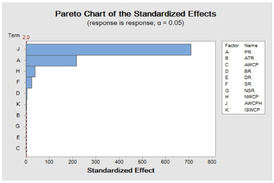
Figure 4.
Pareto diagram of the experiments performed on variables.
As shown in Figure 4, six variables were identified as important variables of the water scarcity system. They are the water consumption rate per cultivated hectare (WCH), infiltration rate in the underground aquifer (PR), birth rate (BR), reduction rate of cultivated area (CDR), consumption rate of non-potable water of person per year (NDCR), and water consumption rate per industrial and service user (WCS). Figure 5 depicts the optimal values of each variable. Notably, the amount of available water will reach 4,878,000,000 m3 if any of the variables reach this level. Different scenarios can be proposed based on these values for each variable. At first, the optimal value of each variable was entered into the stock-flow diagram, and then its effect on the related variable and the response variable was investigated. Ultimately, all variables were entered into the model and the system status was assessed when all the variables reached their optimal level.
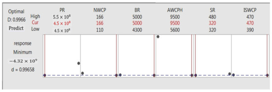
Figure 5.
The optimal amounts of the variables and the response variable.
Step five: The current and optimal states of the variables were compared based on the values obtained in Figure 5, and some solutions were provided to reach the optimal state of the variables.
Five scenarios are provided using Vensim software for better management of water resources and dealing with the water shortage crisis in this city. These scenarios are as follows:
3.1. Results Obtained by the First Scenario
Figure 6 and Figure 7 exhibit the impact of the optimal infiltration rate on the amount of available water and the amount of water balance, respectively. Note that, in Figure 7, Figure 8, Figure 9, Figure 10, Figure 11, Figure 12, Figure 13, Figure 14, Figure 15, Figure 16 and Figure 17, the graphs marked in blue depict the current values, whereas the graphs marked in red represent the optimal values.
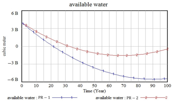
Figure 6.
The influence of the optimal amount of infiltration in the underground aquifers on the amount of available water.
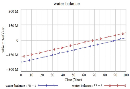
Figure 7.
The influence of the optimal amount of infiltration in the underground aquifers on the water balance.
Note that the penetration of water into the underground aquifers is not very high in the short term. Nevertheless, its effect can gradually increase in the long term, which can delay the crisis of groundwater shortage for 10 to 15 years (i.e., it could delay the arrival time for the amount of available water to reach zero from approximately 20 years to about 30–35 years). Furthermore, it should be mentioned that this variable is affected by the annual rainfall and running water. The only way to obtain this optimal level is to fertilize the clouds for artificial precipitation and artificial penetration into the aquifer, which requires spending a lot of money. On the other hand, infiltration with the same optimal rate can promote the water surplus for wetlands between 20 and 25 years (the time to reach the water surplus is decreased from approximately 90 years to about 67 years, indicating a surpassing of the supply forces over the demand forces).
3.2. Results Obtained by the Second Scenario
Figure 8 and Figure 9 depict the effect of the current and optimal amount of non-potable water consumption per person on the amount of available water as well as the amount of water balance, respectively.

Figure 8.
The effects of the optimal and current amounts for non-potable water consumption per person on the amount of available water.
Figure 8.
The effects of the optimal and current amounts for non-potable water consumption per person on the amount of available water.


Figure 9.
The effect of the optimal amount of non-drinkable water consumption per person on the water balance.
Figure 9.
The effect of the optimal amount of non-drinkable water consumption per person on the water balance.

As shown in Figure 8, the amount of non-potable water consumption by each person has a minor effect on the amount of available water in the short term, whereas it has a relatively slow effect on it in the long term. Accordingly, the effect of policies based on reducing water consumption by households on the amount of available water is not very remarkable. Consequently, it is better to pay more attention to other policies (Figure 9). Nonetheless, regarding this figure, these policies have a better impact on water balance and a relatively better effect on controlling water shortage.
3.3. Results Obtained by the Third Scenario
Figure 10 and Figure 11 illustrate the effect of water consumption per hectare of agricultural land in the current and optimal state on the amount of available water and water balance, respectively.

Figure 10.
The effect of the optimal water consumption per hectare on the amount of available water.
Figure 10.
The effect of the optimal water consumption per hectare on the amount of available water.


Figure 11.
The effect of the optimal amount of water consumption per hectare of the water balance.
Figure 11.
The effect of the optimal amount of water consumption per hectare of the water balance.

According to these figures, the amount of consumption per hectare of agricultural land contains a great effect on the amount of available water as well as the amount of balance (i.e., water shortage). It can be concluded that the best policies in the field of managing the water shortage crisis in this wetland are related to the agricultural sector as well as the reform of this sector. Thus, it is recommended to pay a lot of attention to better managing the water crisis and to activities such as improving irrigation networks, changing cultivation methods, planting crops that need little water, modifying seeds, and other activities leading to decreasing water consumption per hectare.
3.4. Results Obtained by the Fourth Scenario
Figure 12 and Figure 13 show the effect of the optimal reduction of the cultivated area on the amount of available water as well as the water balance, respectively.

Figure 12.
The effect of the optimal amount of reduction in the cultivated area on the amount of available water.
Figure 12.
The effect of the optimal amount of reduction in the cultivated area on the amount of available water.


Figure 13.
The effect of the optimum reduction in the cultivated area on the water balance.
Figure 13.
The effect of the optimum reduction in the cultivated area on the water balance.

Obviously, decreasing the cultivated area did not have a considerable effect on the amount of available water and water balance, since its effect must first be applied to the cultivated area and then to the water consumption, which required passing time. Hence, its effect is not very clear at first but increases little by little as the period becomes longer, indicating a great effect over a very long period of time. It can be concluded that one should not expect much from this variable to manage the water crisis.
3.5. Results Obtained by the Fifth Scenario
Figure 14 and Figure 15 depict the effects of current and optimal water consumption of industry and services on the amount of available water and water balance, respectively.

Figure 14.
The effect of the optimal rate of water consumption of each industrial and service subscriber on the amount of available water.
Figure 14.
The effect of the optimal rate of water consumption of each industrial and service subscriber on the amount of available water.


Figure 15.
The influence of the optimal water consumption rate of each industrial and service user on the water balance.
Figure 15.
The influence of the optimal water consumption rate of each industrial and service user on the water balance.

Note that the rate of water consumption by the service and industrial sectors does not have a considerable effect on the amount of available water as well as on the amount of water balance. The reasons for this issue can be as follows:
- At some times of the year, industrial and service units (i.e., schools, universities, etc.) are closed and do not consume water;
- Industrial and service units pay more attention to the problem of efficiency and effectiveness or productivity in general;
- Industrial and service units have better capital to update water consumption equipment and use facilities for less water consumption.
3.6. The System Describes the Optimality of All Variables

Figure 16.
The state of available water at the time of optimum values of all variables.
Figure 16.
The state of available water at the time of optimum values of all variables.


Figure 17.
The state of water balance at the time of optimum values of all variables.
Figure 17.
The state of water balance at the time of optimum values of all variables.

Based on the obtained results, we assert that the simultaneous application of all policies can prevent the occurrence of a water crisis forever. However, this level requires a lot of money, activities, and time. Moreover, the policies cause water supply forces over the water demand forces, leading to preserving the amount of available water as well as increasing this amount annually.
4. Conclusions and Future Suggestions
This paper simulated the water shortage crisis in Rafsanjan using the system dynamics approach. Some scenarios were developed for better management of water resources and related problems. The scenario of reducing water consumption per hectare of cultivated area was the best. Thus, paying attention to the issue of agriculture and improvement in agricultural activities can be the best solution to prevent the water crisis in this city. The sensitivity of the variables was analyzed based on quantitative values. By providing the obtained results to related organizations such as regional water, and water and sewage companies, it is possible to help better orient and improve future decisions. The following recommendations can be mentioned:
- As the most sensitive variable of the proposed system was the amount of water consumption per hectare of cultivated area, the boundary of the system should be developed by the agricultural sector, in which the factors and variables of the agricultural system should be identified and then optimized.
- This paper utilized a DOE statistical method to determine and optimize the system variables. It is suggested to use other methods such as multi-criteria decision-making (MCDM) techniques to optimize the variables in future studies.
Author Contributions
Conceptualization, N.S.-P., S.B. and A.H.; methodology, N.S.-P. and S.B.; investigation, N.S.-P. and S.B.; visualization, N.S.-P. and S.B.; writing—original draft preparation, N.S.-P. and S.B.; writing—review and editing, N.S.-P., S.B., A.H. and A.F.; supervision, N.S.-P., A.H. and A.F. All authors have read and agreed to the published version of the manuscript.
Funding
This research received no external funding.
Informed Consent Statement
Not applicable.
Data Availability Statement
Not applicable.
Conflicts of Interest
The authors declare no conflict of interest.
References
- Xi, X.; Poh, K.L. Using system dynamics for sustainable water resources management in Singapore. Procedia Comput. Sci. 2013, 16, 157–166. [Google Scholar] [CrossRef]
- Abdiyev, K.Z.; Maric, M.; Orynbayev, B.Y.; Toktarbay, Z.; Zhursumbaeva, M.B.; Seitkaliyeva, N.Z. Flocculating properties of 2-acrylamido-2-methyl-1-propane sulfonic acid-co-allylamine polyampholytic copolymers. Polym. Bull. 2022, 79, 10741–10756. [Google Scholar] [CrossRef]
- Kojiri, T.; Hori, T.; Nakatsuka, J.; Chong, T.S. World continental modeling for water resources using system dynamics. Phys. Chem. Earth Parts A/B/C 2008, 33, 304–311. [Google Scholar] [CrossRef]
- Sun, Y.; Liu, N.; Shang, J.; Zhang, J. Sustainable utilization of water resources in China: A system dynamics model. J. Clean. Prod. 2017, 142, 613–625. [Google Scholar] [CrossRef]
- Zhang, X.H.; Zhang, H.W.; Chen, B.; Chen, G.Q.; Zhao, X.H. Water resources planning based on complex system dynamics: A case study of Tianjin city. Commun. Nonlinear Sci. Numer. Simul. 2008, 13, 2328–2336. [Google Scholar] [CrossRef]
- Kerimkulova, A.R.; Azat, S.; Velasco, L.; Mansurov, Z.A.; Lodewyckx, P.; Tulepov, M.I.; Kerimkulova, M.R.; Berezovskaya, I.; Imangazy, A. Granular rice husk based sorbents for sorption of vapors of organic and inorganic matters. J. Chem. Technol. Met. 2019, 54, 578–584. [Google Scholar]
- Srinivasan, V.; Lambin, E.F.; Gorelick, S.M.; Thompson, B.H.; Rozelle, S. The nature and causes of the global water crisis: Syndromes from a meta-analysis of coupled human-water studies. Water Resour. Res. 2012, 48, W10516. [Google Scholar] [CrossRef]
- Guo, H.C.; Liu, L.; Huang, G.H.; Fuller, G.A.; Zou, R.; Yin, Y.Y. A system dynamics approach for regional environmental planning and management: A study for the Lake Erhai Basin. J. Environ. Manag. 2001, 61, 93–111. [Google Scholar] [CrossRef] [PubMed]
- Ho, C.C.; Yang, C.C.; Chang, L.C.; Chen, T.W. The application of system dynamics modeling to study impact of water resources planning and management in Taiwan. In Proceedings of the 23rd International Conference of the System Dynamics Society, Boston, MA, USA, 17–21 July 2005; pp. 17–21. [Google Scholar]
- Feng, L.H.; Zhang, X.C.; Luo, G.Y. Application of system dynamics in analyzing the carrying capacity of water resources in Yiwu City, China. Math. Comput. Simul. 2008, 79, 269–278. [Google Scholar] [CrossRef]
- Dai, D.; Sun, M.; Lv, X.; Hu, J.; Zhang, H.; Xu, X.; Lei, K. Comprehensive assessment of the water environment carrying capacity based on the spatial system dynamics model, a case study of Yongding River Basin in North China. J. Clean. Prod. 2022, 344, 131137. [Google Scholar] [CrossRef]
- Cheng, L.I. System dynamics model of Suzhou water resources carrying capacity and its application. Water Sci. Eng. 2010, 3, 144–155. [Google Scholar]
- Wei, S.; Yang, H.; Song, J.; Abbaspour, K.C.; Xu, Z. System dynamics simulation model for assessing socio-economic impacts of different levels of environmental flow allocation in the Weihe River Basin, China. Eur. J. Oper. Res. 2012, 221, 248–262. [Google Scholar] [CrossRef]
- Madani, K.; AghaKouchak, A.; Mirchi, A. Iran’s socio-economic drought: Challenges of a water-bankrupt nation. Iran. Stud. 2016, 49, 997–1016. [Google Scholar] [CrossRef]
- Forrester, J.W. Industrial dynamics. J. Oper. Res. Soc. 1997, 48, 1037–1041. [Google Scholar] [CrossRef]
- Rahanandeh, R.; Langroodi, P.; Amiri, M. A system dynamics modeling approach for a multi-level, multi-product, multi-region supply chain under demand uncertainty. Expert Syst. Appl. 2016, 51, 231–244. [Google Scholar] [CrossRef]
- Towill, D.R. Industrial dynamics modelling of supply chains. Int. J. Phys. Distrib. Logist. Manag. 1996, 26, 23–42. [Google Scholar] [CrossRef]
- Chen, C.; Liu, W.; Liaw, S.; Yu, C. Development of a dynamic strategy planning theory and system for sustainable river basin land use management. Sci. Total Environ. 2005, 346, 17–37. [Google Scholar] [CrossRef] [PubMed]
- Vlachos, D.; Georgiadis, P.; Iakovou, E. A system dynamics model for dynamic capacity planning of remanufacturing in closed-loop supply chains. Comput. Oper. Res. 2007, 34, 367–394. [Google Scholar] [CrossRef]
- Turner, B.L.; Menendez, H.M.; Gates, R.; Tedeschi, L.O.; Atzori, A.S. System dynamics modeling for agricultural and natural resource management issues: Review of some past cases and forecasting future roles. Resources 2016, 5, 40. [Google Scholar] [CrossRef]
- Montgomery, D.C. Design and Analysis of Experiments, 8th ed.; Wiley: Hoboken, NJ, USA, 2012. [Google Scholar]


Disclaimer/Publisher’s Note: The statements, opinions and data contained in all publications are solely those of the individual author(s) and contributor(s) and not of MDPI and/or the editor(s). MDPI and/or the editor(s) disclaim responsibility for any injury to people or property resulting from any ideas, methods, instructions or products referred to in the content. |
© 2023 by the authors. Licensee MDPI, Basel, Switzerland. This article is an open access article distributed under the terms and conditions of the Creative Commons Attribution (CC BY) license (https://creativecommons.org/licenses/by/4.0/).