The Role of High Nature Value Farmland for Landscape and Soil Pollution Assessment in a Coastal Delta in China Based on High-Resolution Indicators

Abstract

High nature value farmland (HNVf) plays an important role in improving biodiversity and landscape heterogeneity, and it is effective in curbing soil non-point source pollution and carbon loss in sustainable eco-agricultural systems. To this end, we developed high-resolution (2 m × 2 m) indicators for the identification of potential HNVf based on GF1B remote sensing imaging, including the land cover (LC), normalized difference vegetation index (NDVI), Shannon diversity (SH), and Simpsons index (SI). The statistical results for LC with high resolution (2 m × 2 m) showed that there was 41.05% of intensive farmland in the study area, and the pixel proportion of the HNVf map (above G3) was 44.30%. These HNVf patches were concentrated in the transition zone around the edge of the intensive farmland and around rivers, with characteristics of HNVf type 2 being significantly reflected. Among the real-life areas from Map World, elements (i.e., linear forests, rivers, and semi-natural vegetation etc.) of HNVf accounted for more than 70% of these regions, while a field survey based on potential HNVf patches also exhibited significant HNVf characteristics in comparison with intensive farmlands. In addition, from 2002 to 2020, the total migration distance of the gravity center of intensive farmland in the study area was 7.65 km. Moreover, four landscape indices (patch COH index, landscape division index, SH, and SI) slowly increased, indicating that the species richness and biodiversity were improved. It was also found that a series of ecological protection policies provide effective guarantees for an improvement in species diversity and the development of HNVf in the study area. In particular, the average contents of As, Cr, Cu, Ni, and Zn in the HNVf were 20.99 mg kg⁻¹, 121.11 mg kg⁻¹, 21.97 mg kg⁻¹, 29.34 mg kg⁻¹, and 41.68 mg kg⁻¹, respectively, which were lower in comparison with the intensive farmland soil. This is the first HNVf exploration for landscape and soil pollution assessment in a coastal delta in China, and could provide powerful guidance for the ecological protection of farmland soil and the high-quality development of sustainable agriculture.

1. Introduction

Over the past century, intensification has become the leading way for global farmland to pursue high grain yield [1]. The characteristics of intensive farmland include high-intensity utilization, high carbon emissions, and high chemical inputs (pesticides and chemical fertilizers), which have caused a decline in farmland biodiversity [2,3,4], landscape homogenization [5], cultivated land degradation and abandonment [6], and non-point source pollution [7,8,9]. In recent years, the development goals of some traditional farmlands have changed to sustainable practical value and low-intensity utilization [10,11], which play a key role in maintaining the biodiversity of eco-agricultural ecosystems. The re-identification of these farmlands is important for regional carbon neutrality and microclimate improvement.

In fact, low-intensity farmland has gradually developed into a new concept, high nature value farmland (HNVf), which was devised by the European Union (EU) as a new farmland development framework [12,13]. It emphasizes some characteristics of low-intensity land use, including a high proportion of semi-natural vegetation, a low input of agricultural chemicals, and carbon sequestration. These high nature value (HNV) farmlands have a positive effect on biodiversity improvement and landscape heterogeneity. Currently, HNVf is divided into three types [14,15,16]:

Type 1 is farmland with a high proportion of semi-natural vegetation.

Type 2 is farmland with low-intensity agriculture composed of natural and structural elements, such as field edges, hedgerows, forest land, small rivers, etc.

Type 3 is farmland that supports rare plants and animals, or a high percentage of European or world population farmland (existing in small-scale and centrally managed landscapes).

At present, the identification and evaluation of HNVf relies on various database methods, including the CORINE Land Cover (CLC) database, the farming systems approach (FSA), and the Integrate Administrative and Control System (IACS). The identification and evaluation indicators of HNVf involved in these databases are mainly divided into three categories: land cover (LC), the intensity of farming practices (farm area, production method, livestock, input levels, etc.), and high-precision farm information (farm type, farm area and the number of animals, etc.) [17]. Land cover is the basic indicator of HNVf identification and is regarded as an important representation of the transition from human activity to nature [13]. It describes the artificial gradient of the spatial distribution of natural and semi-natural elements in HNVf by dividing the study area into urban areas, arable lands, forests, wetlands, and other land use types. However, the spatial resolution of the indicator of land cover is low, can only infer the spatial location of potential HNVf, and cannot further obtain other HNVf characteristics in these areas (such as the intensity of agricultural activities), so the identification results have great uncertainty.

The second indicator is the intensity of farming practices, which infers HNVf by introducing factors such as farm area and input levels to identify farmland with low-intensity agricultural characteristics in the area where the accuracy of land cover data cannot be improved [13,15,18]. However, the agricultural activity intensity index from the Farm Accountancy Data Network (FADN) lacks precise localization information for HNVf; that is, if the sample sizes in the area are too small, the identification results have low accuracy. The third indicator is high-precision farm information from IACS [19,20,21], which provides high-precision farm information and parcel-level information updated by EU member states every year, and overcomes the uncertainty of identification results caused by the low spatial resolution of land cover and the shortcomings resulting from missing samples of agricultural activity intensity. However, due to information protection for farmers’ privacy, these indicators are difficult to obtain and cannot be used for the large-scale identification and mapping of HNVf.

Among the above indicators, land cover plays a key role in the identification of HNVf, and its spatial resolution directly affects identification accuracy [14,22]. For example, Maxwell et al. (2017) used the Shannon index (SH) and the Simpson index (SI) for enhancing land cover mapping classification to identify existing HNV and areas with the potential to revert to HNVf type 2 in Wales [23]. In addition, they analyzed the lack of small patches resulting from the low resolution of land cover data, which affects the identification accuracy of HNVf. Bonato et al. (2019) mapped and assessed HNVf and non-HNVf in parts of the Veneto Plain in northeastern Italy in more detail based on the Land Use and Land Cover (LULC) indicator, combining it with information on the intensity of agricultural practices and census data [17]. However, as it is limited to the low spatial resolution of land cover, HNVf is only calculated to the city-level scale. In particular, one shortcoming of the current database methods is their limited use in the EU region, and there are no cases of HNVf identification in China. In China, traditional farmland is facing the challenges of biodiversity loss, non-point source pollution, and carbon loss [9,24,25,26]. For example, at least 60% of arable land (arable non-agricultural land) in China is distributed in ecologically fragile areas, which are very difficult to develop and utilize [5]. He et al. (2017) found that there were a large number of soil pollution cases in China. The development of HNVf is important in addressing these issues [27].

The key way to identify HNVf currently is to develop high spatial resolution land cover data. In recent years, machine learning methods combined with high-resolution remote sensing images were used to classify land use effectively [28], with the advantages of high classification precision and computation speed. The higher the spatial resolution of land cover data, the more significant the characteristics of HNVf in the transition zone. Due to the potential importance and practicality of HNVf identification using land cover indicators, the aim of this study is to confirm the usefulness of identifying potential HNVf with high-resolution data, which has never been done before. Therefore, our objectives are as follows:

(a)

High-resolution (2 m × 2 m) indicators (i.e., LC, NDVI, SH, and SI) are applied for first time to develop a potential HNVf map based on a coastal delta in China;

(b)

The role of the HNVf map in landscape and soil pollution assessment is analyzed.

2. Materials and Methods

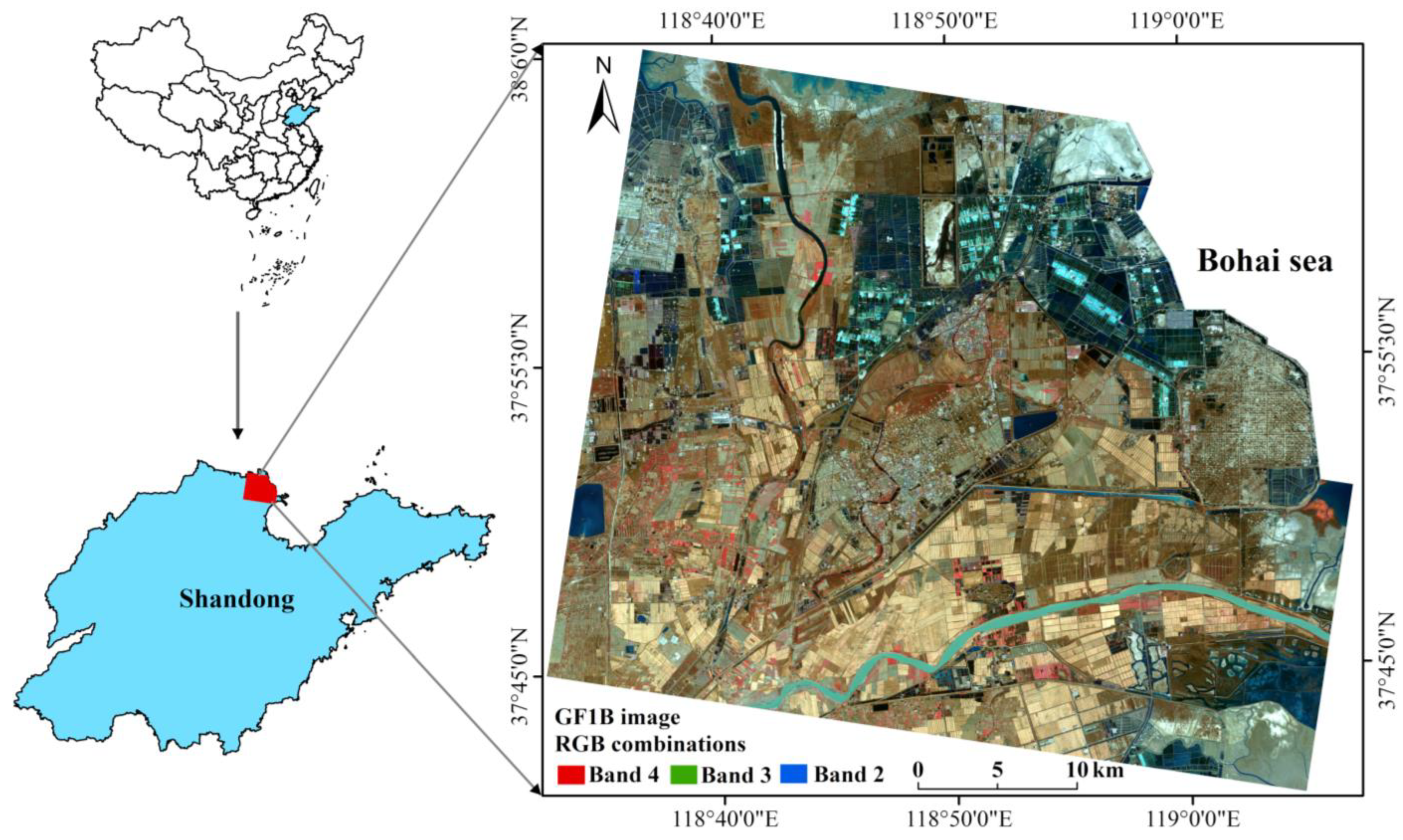
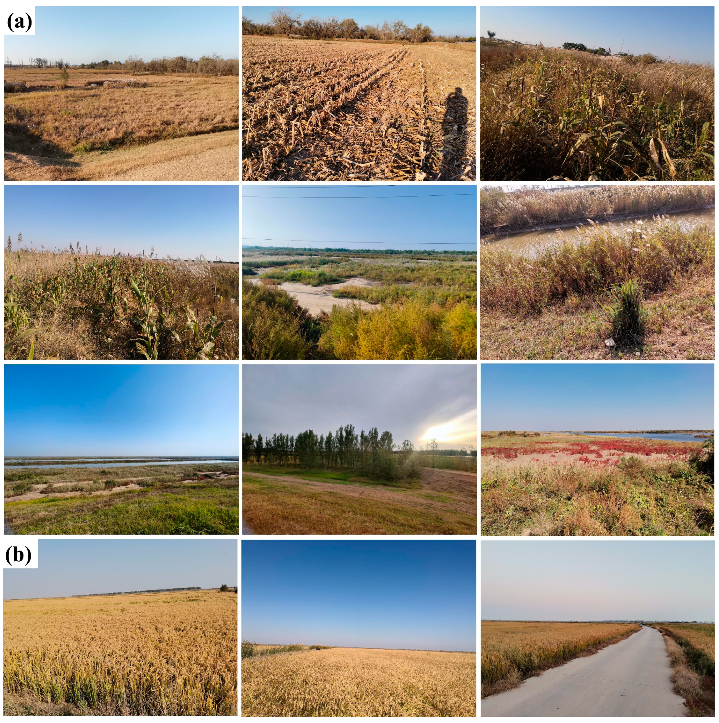
2.1. Study Area

The study area is located in the Yellow River Delta (YRD) in China (39°07′ N–39°42′ N, 116°46′ E–117°19′ E) (Figure 1). It has a semiarid continental monsoon climate, with an average annual temperature of 14.2 °C, an annual average illumination of 2502.3 h, and an average annual precipitation of 628 mm. The YRD has serious soil salinization problems due to the low level of the terrain near the sea, improper irrigation, and other human activities. As a result, the ecology of the YRD has suffered severe damage, which has dramatically restricted the sustainable development of agriculture and the economy in this region. On 16 November 2022, the General Office of Shandong Provincial People’s Government issued the “Support a number of policy measures to promote ecological protection and high-quality development of the Yellow River Basin in 25 counties (cities, districts) along the Yellow River” (http://www.shandong.gov.cn/, (accessed on 25 November 2022)), pointing out the necessity to construct a green ecological corridor in the lower Yellow River, supporting the comprehensive utilization of saline–alkaline land, along with the protection and restoration of wetland ecosystem in the YRD. Therefore, as a natural and semi-natural agricultural system with low-density tillage and various land cover types, HNVf will play a key role in biodiversity protection, ecosystem restoration, and sustainable agricultural development in the YRD.

2.2. Indicators and Auxiliary Data

2.2.1. Land Cover Indicator

Table 1 shows the spatial resolution statistics of the land cover maps used in the study of HNVf identification. The indicators used in these studies all contain land cover data, with the spatial resolution constantly improving from 3 km to 30 m, which shows that the improvement in the spatial resolution of this indicator has a great effect on HNVf. In this study, Landsat 8 operational land imager (OLI) (30 m × 30 m) (10 November 2020) and Gaofen-1B (GF1B) panchromatic multispectral scanner (PMS) (2 m × 2 m) (10 November 2020) images were selected to calculate land cover maps. Over these months, intensive farmland crops are harvested in northern China, with most of the surface being bare soil, which avoids confusion between crops and shrubs or grass. The GF1B PMS image was derived from the natural resource satellite remote sensing cloud service platform (http://www.sasclouds.com/chinese/home/ (accessed on 30 December 2020)), and the Landsat 8 OLI images came from the geospatial data cloud (http://www.gscloud.cn/#page1/1 (accessed on 25 January 2022)). The OLI and PMS image processing steps were as follows:

(1). Radiometric calibration and atmospheric correction were used to preprocess the PMS and OLI images in ENVI 5.3 software, and the panchromatic band from the GF1B satellite was calibrated using ortho-correction;

(2). The preprocessed images were combined with a support vector machine (SVM) algorithm to perform sample selection and supervised classification in ENVI 5.3 software. Overall accuracy and Kappa coefficient of supervised classification for the OLI (94.77% and 0.9027) and PMS images (93.26% and 0.9088) were determined in combination with the validation samples, which exhibited a powerful recognition performance from SVM for land types. Based on existing research [29], land cover data were classified into five classes;

(3). Finally, two land cover maps (2 m × 2 m and 30 m × 30 m) were obtained. The types of LC included built-up area (L1), intensive farmland (L2), woodland and grassland (L3), water body (L4), and semi-natural vegetation (L5) (i.e., shrubs, artificial linear forests, small rivers, ecological ditches, wetlands, and wasteland with herbaceous plants).

Table 1. Spatial resolution of land cover maps on study of HNVf identification.

Study Area	Resolution	Land Cover Types	HNVf Identification Result	Reference
Ireland	2 km × 2 km	Beach, water, pasture, arable land, and shrubs	It represents the most comprehensive method to identify the HNVf	[29]
Estonia	1 km × 1 km	Inland plots, coastline intersection or contact plots, and urban areas	Better recognition in coastal areas, flood plain valleys, and moraine land	[21]
Wales	1 km × 1 km	Semi-natural land	At low-intensity land use, species-rich groups include wetland plants, plant habitat indicators, upland birds, and so on	[30]
France	250 m × 250 m	Semi-natural elements, urban and agricultural areas	All indicators can relate to the dimensions of land use intensity	[31]
Italy	100 m × 100 m	Farmland, non-irrigation arable crops	Better recognition of HNVf type 3	[32]
Italy	50 m × 50 m	Urban fabric, arable lands, permanent crops, pastures, and heterogeneous agricultural areas	Compared to traditional land cover map, agricultural statistics improved the identification results of HNVf	[17]
United Kingdom	30 m × 30 m	The UK Biodiversity Action Plan Broad Habitats	Land cover type have been the main data used for reporting but no consistent set of data metrics have been agreed	[23]

Table 1. Spatial resolution of land cover maps on study of HNVf identification.

Study Area	Resolution	Land Cover Types	HNVf Identification Result	Reference
Ireland	2 km × 2 km	Beach, water, pasture, arable land, and shrubs	It represents the most comprehensive method to identify the HNVf	[29]
Estonia	1 km × 1 km	Inland plots, coastline intersection or contact plots, and urban areas	Better recognition in coastal areas, flood plain valleys, and moraine land	[21]
Wales	1 km × 1 km	Semi-natural land	At low-intensity land use, species-rich groups include wetland plants, plant habitat indicators, upland birds, and so on	[30]
France	250 m × 250 m	Semi-natural elements, urban and agricultural areas	All indicators can relate to the dimensions of land use intensity	[31]
Italy	100 m × 100 m	Farmland, non-irrigation arable crops	Better recognition of HNVf type 3	[32]
Italy	50 m × 50 m	Urban fabric, arable lands, permanent crops, pastures, and heterogeneous agricultural areas	Compared to traditional land cover map, agricultural statistics improved the identification results of HNVf	[17]
United Kingdom	30 m × 30 m	The UK Biodiversity Action Plan Broad Habitats	Land cover type have been the main data used for reporting but no consistent set of data metrics have been agreed	[23]

2.2.2. Vegetation Indicator

The vegetation index is an important indicator used to characterize HNVf type 2 (field edges, hedgerows, woodlands or bushes, etc.), and it is also critical for accurately identifying the location of HNVf. However, there are two challenges in extracting this vegetation information. On the one hand, the spatial resolution of a land cover map can clearly express vegetation features. On the other hand, confusing vegetation information with farm crops should be avoided. In particular, the normalized difference vegetation index (NDVI) contains more information on woodland, bush, grass, and wetland plants, which could ideally reflect the spatial location of HNVf. In order to ensure the high resolution of the vegetation index, the GF1B panchromatic band and the PMS multi-band images were fused based on the NNDiffuse pan-sharpening algorithm in ENVI 5.3 software, and then a multi-band image with a resolution of 2 m × 2 m was obtained. The NDVI was calculated based on the near-infrared (NIR) and infrared (R) bands (Equation (1)) of the preprocessed OLI images (30 m×30 m) and GF1B image (2 m × 2 m) [33]:

NDVI = (NIR − R)/(NIR + R)

(1)

2.2.3. Richness Indicator

Species richness (such as insects, birds, etc.) is an important indicator for distinguishing between intensive farmland and HNVf. However, the traditional rich data acquisition method requires field observation, which takes a lot of time and is high in cost. The landscape index can highlight the macro-distribution of different populations in the region, which could play a significant role in identifying HNVf. We selected two landscape indices (SH and SI) as the identification indicators of HNVf. Among them, SH (Equation (2)) is one of the most commonly used indicators to measure biodiversity [34]. It estimates the average uncertainty regarding the type of land cover a random pixel belongs to, and is especially sensitive to the non-equilibrium distribution of each land cover type, emphasizing the contribution of rare objects to biodiversity information. SI (Equation (3)) is a comprehensive index that can describe uniformity and richness [35]. Since SI is less affected by the type of rare land cover, it is more inclined to express evenness.

$$SH={\displaystyle \sum }_{i=1}^s{p}_i\begin{array}{c}ln{p}_i\end{array}$$

(2)

$$SI={\displaystyle \sum }_{I=1}^S{p}_i{}^2$$

(3)

where s represents the total number of land cover types and $p_i$ is the proportion of the total area of the ith land cover type. Based on the land cover maps from the OLI and GF1B remote sensing images, the SH and SI, respectively, were calculated using FRASTATICS 4.2.1 software. In addition, in order to unify the levels of indicators in the process of weighted superposition, we normalized the levels of NDVI, SH, and SI maps from 1 to 5 using a grid calculator and the natural breakpoint methods in ArcGIS 10.6 software.

2.2.4. Soil Sampling Data

In order to quantify the soil characteristics of HNVf and non-HNVf, soil heavy metal was selected for a comparative analysis of the identified HNVf maps. Based on the potential HNVf map, we collected 64 soil samples (40 in HNVf regions and 24 in non-HNVf regions). Approximately 1 kg of soil samples were collected and GPS coordinates were recorded. The physical treatment of all samples included indoor air drying, crushing and grinding, and passing through 200-mesh nylon sieves. Amounts of 6 mL HNO₃, 2 mL HCl, and 2 mL HF were added to the pretreated samples according to the proportion of 3:1:1. A GSS-1 standard soil sample and a blank were added to each batch of samples. After microwave digestion, the soil samples were measured on an inductively coupled plasma mass spectrometer (Agilent 7500ce, SC, CA, USA). Finally, the measured contents of As, Cr, Cu, Ni, and Zn in the study area were obtained.

2.2.5. Migration Distance and Landscape Index

To explore the effect of spatiotemporal variations in intensive farmland for HNVf in the study area, we collected Landsat satellite time series images from 2002 to 2020 (

Table 2. Images of Landsat satellites and classification accuracy using SVM from 2002 to 2020.

Sensor	Time	Accuracy	Sensor	Time	Accuracy
ETM+	15 October 2002	90.69%	ETM+	27 November 2012	93.52%
ETM+	21 November 2004	90.10%	OLI	9 November 2014	94.56%
ETM+	11 November 2006	91.15%	OLI	30 November 2016	94.88%
ETM+	18 December 2008	92.40%	OLI	20 November 2018	93.25%
ETM+	8 December 2010	91.51%	OLI	10 November 2020	94.77%

). The SVM was used to classify the Landsat Enhanced Thematic Mapper Plus (ETM+) and OLI images, as well as the extracted intensive farmland information. The migration distance of the center of gravity of intensive farmland was then calculated from 2002 to 2020. The formula (Equation (4)) for the center of gravity is [36]:

$$\overline{x}=\frac{{{\displaystyle \sum }}_{j=1}^n{T}_j{X}_j}{{{\displaystyle \sum }}_{j=1}^n{T}_j}\begin{array}{c}\overline{y}=\frac{{{\displaystyle \sum }}_{j=1}^n{T}_j{Y}_j}{{{\displaystyle \sum }}_{j=1}^n{T}_j}\end{array},$$

(4)

where $\overline{x}$ and $\overline{y}$ denote the longitude and latitude of the coordinates of the center of gravity of farmland in the study area; n is the number of secondary units; $X_j$ and $Y_j$ represent the geographic center coordinates of the jth subunit; and $T_j$ represents a property value for a range. The center of gravity coordinates can be used to calculate the moving distance of farmland in the space. The center of gravity analysis was implemented using ENVI 5.3 software.

In addition, the landscape index indirectly reflects the spatiotemporal evolution of HNVf through the description of regional biodiversity and the degree of human activity. Based on the results of land cover, four landscape indices from 2002 to 2020 were calculated in the FRASTATICS 4.2 software, including the patch COH index (COH) [37], the landscape division index (DIS) [38], SH, and SI.

2.3. Weight and Verification

We assigned different weights to LC, NDVI, SH, and SI, based on existing studies [29]. For example, Paracchini et al. (2008) [15] and Sullivan et al. (2013) [39] used semi-natural habitat coverage as a direct indicator of HNVf and assigned it maximum weight (45%). Therefore, this study set the weight of LC to 45%, ensuring that the weight allocation results were similar to those of other studies. The weight of NDVI was 25%, reflecting the characteristics of shrubs, grassland, and forest within the boundary of the field as much as possible. The SH and SI weights were both 15%, reflecting high levels of semi-natural habitat, species diversity, and block boundary.

The verification of the HNVf identification result is relatively diversified. Many studies ascertain whether the identification results conform to the characteristics of HNVf based on HNV theory without quantitative verification. This is due to the lack of real validation data; it is difficult to obtain an HNVf identification patch from high-resolution real images. Recently, real-life data from Google Maps has been proven to be effective for verifying HNVf maps [17]. In this study, the results of potential HNVf identification are quantified using Map World real-life data (https://www.tianditu.gov.cn/ (accessed on 15 October 2022)) and field surveys. Map World integrates enormous basic geographic information resources such as 0.6 m resolution remote sensing images, built by the National Administration of Surveying, Mapping and Geoinformation. Six regions were randomly selected in the potential HNVf map to verify whether the HNVf identification result was accurate. In order to overlay a range of verification regions between the Map World images and the HNVf map, we unified the coordinate system as WGS_1984_Web_Mercator_Auxiliary_Sphere. In addition, we also conducted a field survey based on potential HNVf patches in the study area and compared the differences between high-potential HNVf elements and intensive farmlands.

3. Results

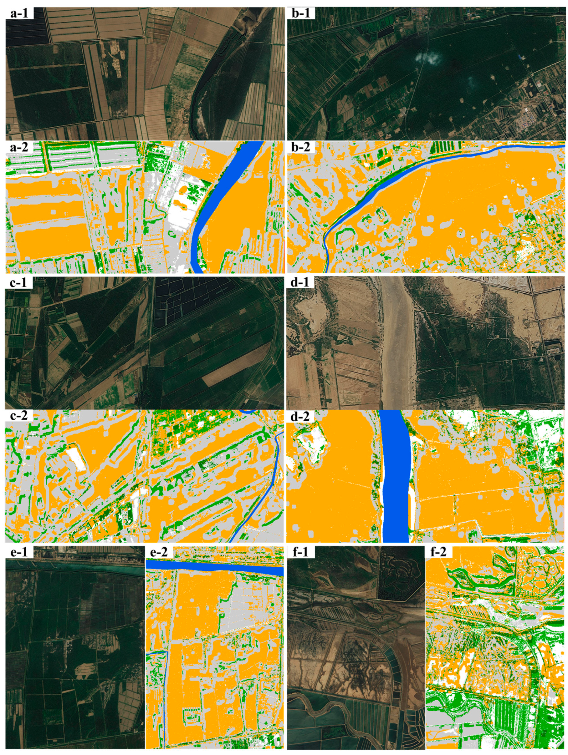
3.1. Land Cover across YRD

Based on LC results from two resolution types (2 m × 2 m and 30 m × 30 m), the pixel proportions of five types (i.e., built-up area, intensive farmland, woodland and grassland, water body, and semi-natural vegetation) were counted (Figure 2a). According to the statistical result of LC with high resolution (2 m × 2 m), intensive farmland made up 41.05% of the study area. Woodland and grassland, water bodies, and semi-natural vegetation were widely distributed (39.47% of which were above L3), indicating that there was a strong HNVf development potential in the study area. The statistical result of LC with low resolution (30 m × 30 m) was similar to that of LC with high resolution. However, there was a large difference between built-up area and semi-natural vegetation, which may have been affected by the pixel resolution. In general, intensive agriculture was the main land cover type in the study area, followed by woodland and grassland and semi-natural vegetation. The LC map with high resolution provided a more accurate description of each land cover type.

3.2. High Nature Value Farmlands across the YRD

The HNVf map was obtained using the weighted superposition of LC, NDVI, SH, and SI in the YRD (Figure 3). Grade 1 and grade 2 (white patches) indicated the non-HNVf (i.e., built-up area and intensive farmland), and these patches did not exhibit features of HNV. Orange and green patches (above grade 3) were considered a high likelihood of HNVf, including HNVf type 1 and HNVf type 2. According to the HNVf maps with two types of resolution (2 m × 2 m and 30 m × 30 m), the pixel proportions of the five grades were counted (Figure 2b). The statistical results of the two HNVf maps were similar, with pixel proportions (above G3) of 43.02% and 44.3%, respectively. The spatial distribution of HNVf type 2 was focused on the edge of intensive farmland and its transition zone with rivers, and these patches were fragmented and scattered. The patches of HNVf were larger and more concentrated around estuaries in the north and the east of the study area.

Compared with the low-resolution HNVf map (30 m × 30 m), the high-resolution HNVf map (2 m × 2 m) better described the edge of intensive farmland and its transition zone. For example, the G3 patches in the low-resolution HNVf map were observed in both the north and the east of the study area, whereas these patches in the high-resolution HNVf map had a gradient and transitional feature from G3 to G5, showing that high-resolution indicators described HNVf more accurately. In addition, the high-resolution HNVf map could extract more refined patches on the edge of intensive farmland and its transition zone. Furthermore, these patches exhibited significant characteristics of HNVf type 2 (spotted and linear distribution) between woodland and intensive farmland, which is consistent with the real distribution. In fact, the real distribution of HNVf was a slow transition from intensive farmland to natural vegetation. In particular, the statistical results of the HNVf pixels showed a similar trend to the proportion of LC pixels, indicating that the LC indicator plays an important driving role in HNVf identification.

3.3. Validation of the HNVf Map

According to the comparison results of the Map World real data corresponding to the selected HNVf areas, the farmland in all regions showed significant HNV characteristics (Figure 4). Elements (i.e., linear forests, rivers, and semi-natural vegetation, etc.) of HNVf accounted for more than 70% of these regions. Among these validation areas, elements of HNVf were prominent in the field edges and in the transition zone between forest and intensive farmland (Figure 4a–c). These landscape patches contained linear forests, shrubs, rivers, and semi-natural vegetation, which exhibited high potential for HNVf type 2. Figure 4d–f show that the proportion of semi-natural vegetation landscape was higher (more than 80%) than for other verification areas, and only sporadic fields were distributed, so these areas had significant high-intensity HNVf characteristics. The dominant HNVf in the study area was type 2, that is, the intensive farmland edge, and its transition landscapes with forests and rivers were distributed on almost all urban surfaces in the region. The Map World real data could effectively verify the characteristics of HNVf. The study area had good HNVf and potential HNVf, and there was less interference from intensive farmland.

In addition, some of the field survey pictures based on the identified HNVf patches are shown in Figure 5. Ten pictures of potential HNVf patches from the field survey showed rich elements of HNVf, such as linear forests, shrubs, grasslands, and small rivers (Figure 5a), exhibiting significant differences compared with intensive farmland (Figure 5b). Particularly near the coastline, semi-natural vegetation is the dominant landscape type, whereas farmland is extremely scarce. As a reliable verification method, field surveys are an effective way to overcome the uncertainty of real-life data from high-resolution remote sensing images for identified HNVf maps.

4. Discussion

4.1. Indicator Characteristics and Development Potential of HNVf

LC is not only a proxy indicator of farming systems intensity [24,40], but it is also the most basic indicator for the identification of HNVf in comparison with other indicators. LC is usually limited to low spatial resolution, which cannot improve the identification accuracy of HNVf. The NDVI can reflect hedgerows, grass slopes, and tree lines [41,42], further demonstrating HNVf feature information. It can be used as a good supplementary indicator to improve the identification accuracy of HNVf, such as fences and shrubs in patches, and to compensate for the spatial resolution shortcomings of land cover classification. In fact, vegetation data have been applied at local scales [43,44].

However, it is difficult to identify rare objects at intensive farmland edges and transition zones using LC and NDVI, whereas SH and SI are particularly influenced by rare objects [23]. SH and SI are used as the basic and most common measures of diversity, largely because of the simplicity and intuitiveness of the concept [45,46]. For example, auxiliary indicators based on the Shannon Evenness Index (SEI) were considered to improve the accuracy of the HNVf assessment analysis [20,47]. SH and SI accurately express a measure of the variability (heterogeneity) in LC within a small neighborhood, which indicates that SH and SI are very effective for the expression of potential HNVf characteristics at intensive farmland edges and transition zones.

The dominant HNVf in the study area is type 2, based on the HNVf map. HNVf type 2 can be seen as a transition between type 1 and type 3. Typically, HNVF type 1 (i.e., semi-natural vegetation) is most easily described, while HNVf type 3 is most easily ignored [48]. This is due to the lack of indicators corresponding to HNVf type 3. Some habitat characteristics of rare animals (such as the crested ibis, golden monkey, and other large marine animals) are difficult to obtain. HNVf type 2 superimposes the HNV features of both type 1 and type 3 transition regions, exhibiting the uncertainty of the HNVf map. For example, the southeastern corner of the study area is the “Shandong Yellow River Delta National Nature Reserve”, which has a clear HNVf type 3 but is mixed with type 2 characteristics.

In this study, we developed a set of minimum common indicators for identifying HNVf in plains areas. However, in order to accurately assess the development potential of HNVf in other regions with different geographical environment conditions, the climate, terrain, biological species, and soil of the region also need to be further considered. For example, climatic conditions have a greater impact (through crop type, soil structure, and crop growth cycle) on farmland from the aspects of precipitation, temperature, humidity, and light. Climate changes such as increased temperature and precipitation affect the growth of vegetation, thus affecting the soil hydrothermal conditions, organic matter content, and formation and development [49]. Ouyang et al. (2017) also showed that, in rice-growing areas, an increase in temperature promotes the expansion of paddy field areas in horizontal and vertical directions [50]. In some scenarios, climatic conditions may be extremely important indicators for the evaluation of the development potential of HNVf. It is essential to consider the impact of other indicators in western China, and the topographic relief and climatic conditions caused by land cover significantly affect the identification accuracy of the HNVf map.

HNVf is a new type of sustainable ecological agriculture, which is reflected in two aspects: ecological technology and policy management. On one hand, many studies have developed ecological technologies such as microbial fertilizers and environmentally friendly fertilizers to promote the development of sustainable agriculture by reducing the utilization intensity of agricultural soil [51,52], which is consistent with the original intention of HNVf [53]. On the other hand, the formulation of farmland protection policies needs to evaluate the value of farmland from many perspectives, and HNVf can provide support for the deep excavation of the natural value of farmland and the multi-dimensional evaluation of farmland quality, as well as contributing a scientific basis and theoretical support for the establishment of a sound farmland protection system [54]. In terms of sustainable agricultural development in China, HNVf is of great significance for the optimization of agricultural structure layout, improvement in the quality of agricultural development, and the structural reform of agricultural supply [55]. Although China has established a strict system for farmland protection, it is necessary to strengthen the formulation and implementation of the laws related to sustainable agricultural development [56]. HNVf also has an impact on policy changes, while policies affect the spatial distribution and time changes in HNVf. Overall, sustainable ecological agriculture can provide scientific and effective guidance for the identification and development of HNVf in terms of improvement measures for low agricultural intensity and ecological cycle protection.

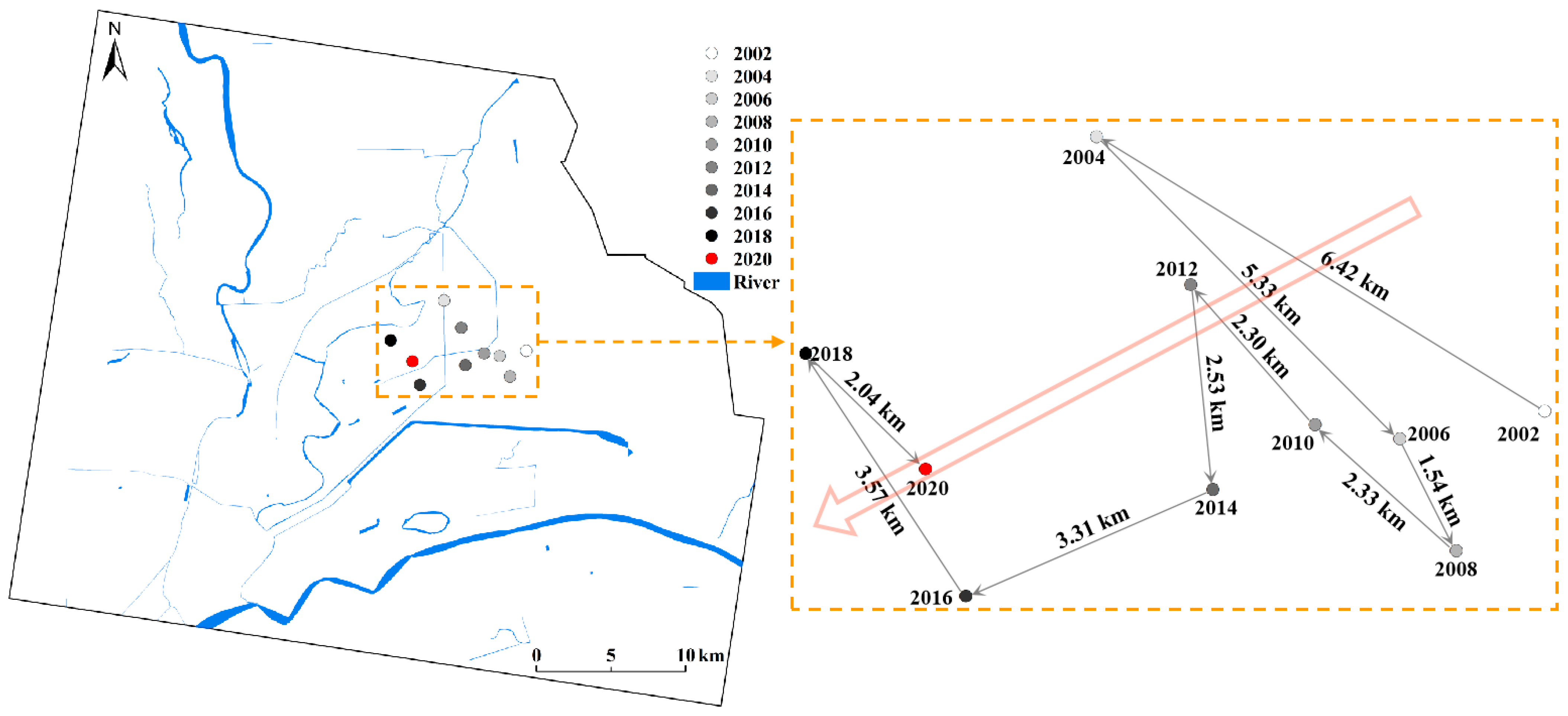
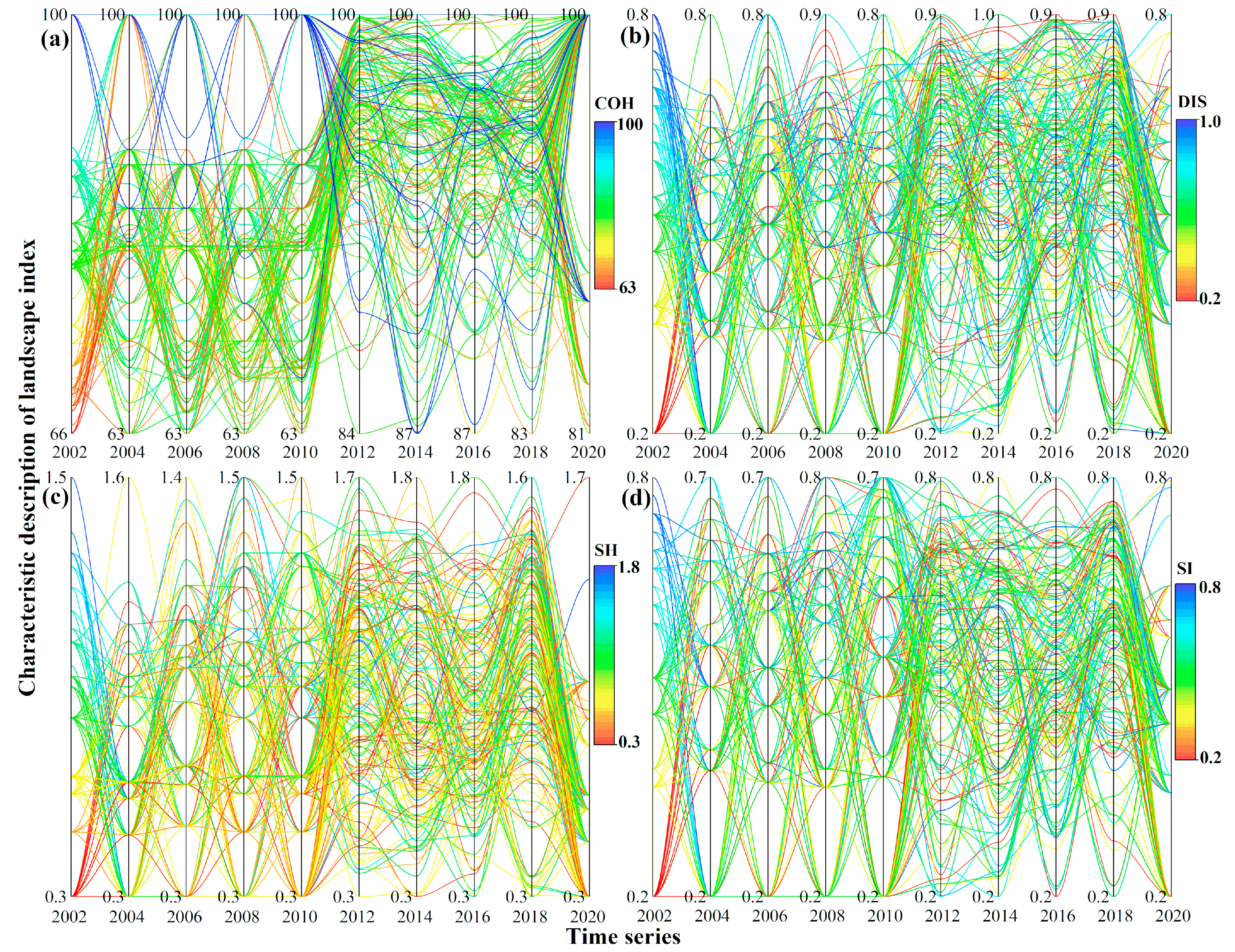
4.2. Effect of Spatiotemporal Evolution of Intensive Farmland on HNV

Figure 6 shows the gravity center migration of intensive farmland in the study area from 2002 to 2020, and the migration distances in turn were 6.42 km, 5.33 km, 1.54 km, 2.33 km, 2.30 km, 2.53 km, 3.31 km, 3.57 km, and 2.04 km. The migration distance of the gravity center of intensive farmland in the study area exhibited a trend of slowing expansion, and the total migration distance from 2002 to 2020 was 7.65 km. The migration direction of the gravity center of intensive farmland was from northeast to southwest. This may be due to the decrease in the sediment deposition rate in the estuary. The deposition rate of estuary sediment drastically declined from 2007 to 2018 [57]. For this reason, the inland areas that can benefit from riverine flow upstream increased [58], and the increased sediment and water input, as well as land reclamation projects, increased the water accessibility of inland areas [59]. Then, the migration direction of the gravity center of intensive farmland was from the coastline to inland. In other words, the intensive farmland was farther away from the coastline, indicating that the ecological protection of the study area was strengthened.

In addition, the characteristic description of four landscape indices from 2002 to 2020 are shown in Figure 7. The parallel trends of COH and SH were similar, exhibiting a fluctuation change and a slow increase after 2010, and indicating that the species richness and biodiversity in the study area improved (Figure 7a,c). Changes in the DIS and SI were smoothed out, indicating that the patch dispersion and species evenness in the study area were less influenced by urbanization and human activity after 2010 (Figure 7b,d). The landscape index results indicated that the biodiversity and landscape heterogeneity in the study area increased significantly after 2010. In addition, the response to the characteristics of HNVf elements (semi-natural vegetation, linear forest, hedgerows, and rivers) is very strong. Due to the implementation of environmental policies from 2006 to 2018, a north–south direction (near the coastline) of wetland area development was increased in the study area [60]; that is, the spatial distribution of HNV areas became more extensive, and the proportion of semi-natural vegetation became more balanced.

In 2009, the State Council of the People’s Republic of China formally approved an instructive document on the plan for developing the Yellow River Delta into an efficient and ecological economic zone, with the ecological protection of the YRD becoming a national strategy. In 2021, the Communist Party of China Central Committee and the State Council jointly issued a document outlining the ecological protection and high-quality development of the Yellow River Basin, which pointed out that the natural extension trend of the YRD coastline should be restored; the protection of biological species resources in salt marshes, tidal flats, and wetlands of estuary shallow seas should be strengthened; and the use of unconventional water sources to supply bird habitats should be explored. Then, in 2022, the Ministry of Ecology and Environment of the People’s Republic of China issued a document outlining the 14th five-year ecological protection supervision plan, which also emphasized that the YRD has a rich biodiversity. It is a migration transfer point and a habitat for rare and endangered birds, making it an important area for the protection of wetland ecosystem biodiversity. A series of ecological and environmental protection measures provide effective guarantees for the restoration of species diversity in the study area. These policies have a positive impact on the development of HNVf.

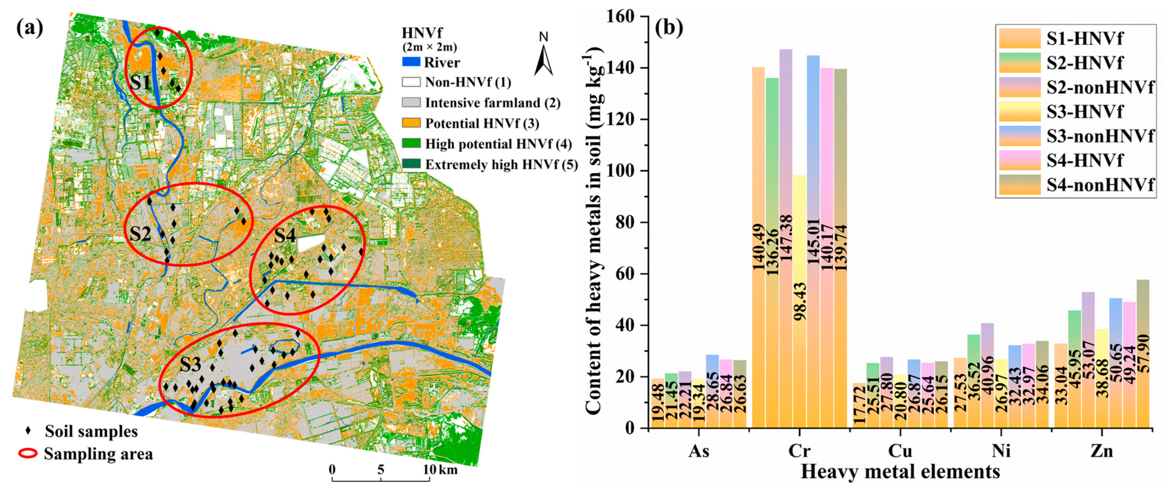
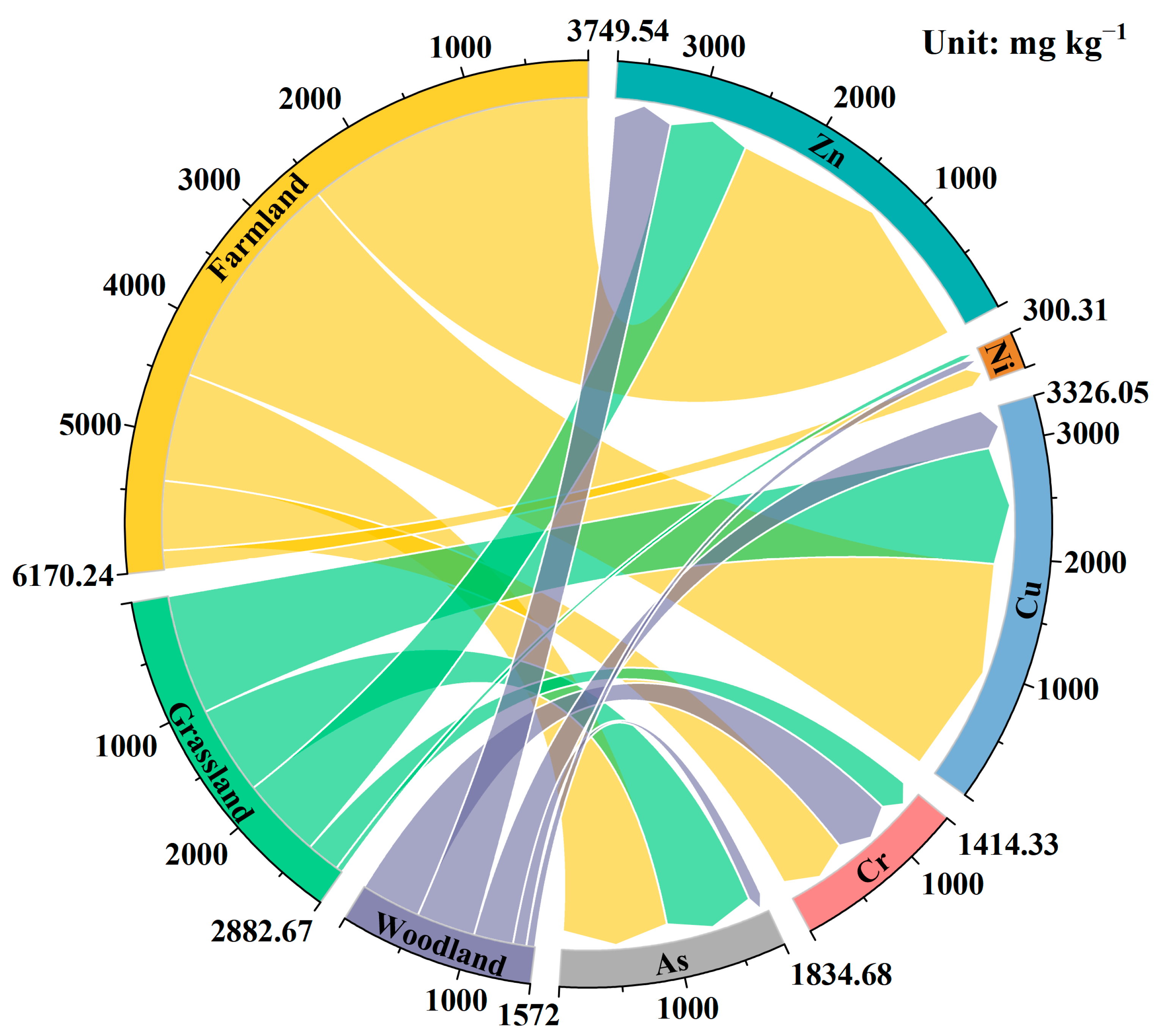
4.3. Characterization of Soil Heavy Metals in the HNVf and Non-HNVf

Figure 8 shows the statistical results of the soil heavy metal content in the HNVf and non-HNVf regions. The average contents of As, Cr, Cu, Ni, and Zn in the HNVf were 20.99 mg kg⁻¹, 121.11 mg kg⁻¹, 21.97 mg kg⁻¹, 29.34 mg kg⁻¹, and 41.68 mg kg⁻¹, respectively (Figure 8). Compared with the intensive farmland (non-HNVf), the soil heavy metal content of the HNVf area was lower. The numerical distribution showed that the values of As, Cu, and Zn in the non-HNVf region were concentrated in the high-value region and were greatly affected by human activities. Furthermore, we counted the content of soil heavy metal in the high semi-natural vegetation area (S1), the transition area from intensive farmland to the river (S2 and S3), and the edge area of the farmland (S4) (Figure 9a). All heavy metals (except Cr and Ni) in S1 were lower in comparison with other HNVf areas, and minimum values of As, Cr, Cu, Ni, and Zn were in S3-HNVf (19.48 mg kg⁻¹), S3-HNVf (98.43 mg kg⁻¹), S1-HNVf (17.72 mg kg⁻¹), S3-HNVf (26.97 mg kg⁻¹), and S1-HNVf (33.04 mg kg⁻¹), respectively. In the S4 area, the heavy metal content in the HNVf soil was also low, and was very close to that of non-HNVf soil (Figure 9b).

Studies on the soil heavy metal content in intensive farmland and other land use types (woodlands, grasslands, etc.) are shown in Figure 10. The highest accumulation levels of heavy metals in intensive farmland, grassland, and woodland soils were Zn (2527.02 mg kg⁻¹), Cu (1050.04 mg kg⁻¹), and Cr (522.20 mg kg⁻¹) (Figure 10). Compared with woodland and grassland soils, intensive farmland soils had the highest accumulation concentrations of As (942.34 mg kg⁻¹), Cr (601.11 mg kg⁻¹), Cu (1932.11 mg kg⁻¹), Ni (167.66 mg kg⁻¹), and Zn (2527.02 mg kg⁻¹), which is consistent with the result of this study, indicating that intensive farmland regions are strongly influenced by human activities (agrochemical inputs and sewage irrigation) [61,62]. A large number of pesticides and fertilizers are applied to farmland, which usually contain high concentrations of Cu and Zn [63]. The topsoil of farmlands is affected by agricultural chemicals, and the mean values of As, Cu, Cd, N, K, P, OM, and Zn were significantly higher than those of grasslands [63,64,65]. In addition, the accumulation of Cd and Zn in farmland around the smelter may also come from surface runoff and atmospheric deposition. The woodland has a dense vegetation canopy to intercept the atmospheric deposition from the smelter, so its soil heavy metal content was low [66]. The Cr content in the intensive farmland and woodland soils and the As content in the grassland soils were similar (Figure 10). This may be because As and Cr are derived from terrestrial (rock and soil) weathering, with greater uncertainty in different land cover types [67].

In addition, similar studies also found that the sources of soil heavy metals in the YRD could be divided into natural sources and human sources [68,69,70]. Natural sources including silicate- and oxide-based parent materials, through weathering, caused soil heavy metal content changes [68]. That is, the sediment transport and deposition of the Yellow River from the Loess Plateau implies that this is the main reason for the redistribution and deposition of heavy metals in the YRD [69]. Human sources include the applications of agrochemicals and fertilizers, the atmospheric deposition of coal combustion, the artificial input of wastewater, industrial emissions, and oil exploitation [71,72]. The HNVf soil at the edge of the farmland in this study was significantly influenced by human activities, which was also the key reason for the heavy metal content being similar to that of intensive farmland soil. In this study, the selected high-resolution indicators reflected the principle of easy access and strong representativeness for the identification of HNVf type 2. Particularly, these indicators were effective for the HNVf identification of farmland edges and transition zones in the study area. The HNVf not only reflects the economic value of intensive farmland, but also exhibits natural value and ecological value. On the whole, the HNVf provides a great deal of potential guidance for the development and protection of farmland biodiversity, landscape heterogeneity, the bearing capacity of soil ecosystem, and carbon sequestration in regional HNVf areas in China.

5. Conclusions

In this study, we developed high spatial resolution indicators (LC, NDVI, SH, and SI) to identify and map potential HNVf in the YRD in China. The proportion of HNVf type 2 characteristics was over 40% in the study area, and real-life images and a field survey based on potential HNVf patches also exhibited significant HNVf characteristics (i.e., linear forests, rivers, and semi-natural vegetation, etc.). These areas were concentrated in the north, the east, and the transition zones of intensive farmlands. In particular, the total migration (7.65 km) of the gravity center of intensive farmland moved inland from the coastline, and the landscape indices slowly increased from 2002 to 2020, exhibiting larger patches of HNVf and higher proportions of semi-natural vegetation around the estuaries in the north and the east of the study area. Furthermore, the intensive farmland was significantly influenced by human activities (agrochemicals inputs and sewage irrigation) in the study area, with the soil heavy metal content found to be higher than that in the HNVf areas (i.e., the high semi-natural vegetation area, the transition area from intensive farmland to the river, and the edge area of intensive farmland). In the future, soil heavy metal can be regarded as a potential indicator for the accurate identification of different types of HNVf, which supports the high-quality development of sustainable farmland and provides powerful guidance for ecological protection policies.

References

1. Wade, M.R.; Gurr, G.M.; Wratten, S.D. Ecological restoration of farmland: Progress and prospects. Phil. Trans. R. Soc. B Biol. Sci. 2008, 363, 831–847. [Google Scholar] [CrossRef] [PubMed]
2. Flandroy, L.; Poutahidis, T.; Berg, G.; Clarke, G.; Dao, M.; Decaestecker, E.; Furman, E.; Haahtela, T.; Massart, S.; Plovier, H. The impact of human activities and lifestyles on the interlinked microbiota and health of humans and of ecosystems. Sci. Total Environ. 2018, 627, 1018–1038. [Google Scholar] [CrossRef] [PubMed]
3. Xu, D.; Li, D. Variation of wind erosion and its response to ecological programs in northern china in the period 1981–2015. Land Use Policy 2020, 99, 104871. [Google Scholar] [CrossRef]
4. Wang, H.; Zhang, C.; Yao, X.; Yun, W.; Ma, J.; Gao, L.; Li, P. Scenario simulation of the tradeoff between ecological land and farmland in black soil region of northeast china. Land Use Policy 2022, 114, 105991. [Google Scholar] [CrossRef]
5. Penghui, J.; Manchun, L.; Liang, C. Dynamic response of agricultural productivity to landscape structure changes and its policy implications of Chinese farmland conservation. Resour. Conserv. Recy. 2022, 156, 104724. [Google Scholar] [CrossRef]
6. Ma, L.; Long, H.; Tu, S.; Zhang, Y.; Zheng, Y. Farmland transition in China and its policy implications. Land Use Policy 2020, 92, 104470. [Google Scholar] [CrossRef]
7. Liu, M.; Jia, Y.; Cui, Z.; Lu, Z.; Zhang, W.; Liu, K.; Shuai, L.; Shi, L.; Ke, R.; Lou, Y. Occurrence and potential sources of polyhalogenated carbazoles in farmland soils from the three northeast provinces, china. Sci. Total Environ. 2021, 799, 149459. [Google Scholar] [CrossRef]
8. Zhang, Q.; Wang, Y.; Jiang, X.; Xu, H.; Luo, Y.; Long, T.; Li, J.; Xing, L. Spatial occurrence and composition profile of organophosphate esters (opes) in farmland soils from different regions of china: Implications for human exposure. Environ. Pollut. 2021, 276, 116729. [Google Scholar] [CrossRef]
9. Hu, J.; He, D.; Zhang, X.; Li, X.; Chen, Y.; Wei, G. National-scale distribution of micro(meso)plastics in farmland soils across china: Implications for environmental impacts. J. Hazard. Mater. 2022, 424, 127283. [Google Scholar] [CrossRef]
10. Barnes, A.P.; Thomson, S.G. Measuring progress towards sustainable intensification: How far can secondary data go? Ecol. Ind. 2014, 36, 213–220. [Google Scholar] [CrossRef]
11. EC-European Commission. Report from the Commission to the European Parliament and the Council the Mid-Term Review of the EU Biodiversity Strategy to 2020; EC-European Commission: Brussels, Belgium, 2015. [Google Scholar]
12. Clark, J.; Beaufoy, G.; Baldock, D. The Nature of Farming: Low Intensity Farming Systems in Nine European Countries; Institute for European Environmental Policy: Brussels, Belgium, 1994. [Google Scholar]
13. Andersen, E.; Baldock, D.; Brouwer, F.M.; Elbersen, B.S.; Godeschalk, F.E.; Nieuwenhuizen, W.; van Eupen, M.; Hennekens, S.M.; Zervas, G. Developing a High Nature Value Farming Area Indicator; Internal Report for the European Environment Agency; Institute for European Environmental Policy: Brussels, Belgium, 2004. [Google Scholar]
14. IEEP. Guidance Document to the Member States on the Application of the High Nature Value Indicator; IEEP: Brussels, Belgium, 2007. [Google Scholar]
15. Paracchini, M.L.; Petersen, J.; Hoogeveen, Y.; Bamps, C.; Burfield, I.; van Swaay, C. High Nature Value Farmland in Europe. An Estimate of the Distribution Patterns on the Basis of Land Cover and Biodiversity Data; European Commission: Brussels, Belgium, 2008; p. 23480. [Google Scholar]
16. Keenleyside, C.; Beaufoy, G.; Tucker, G.; Jones, G. High nature value farming throughout eu-27 and its financial support under the cap. Inst. Eur. Environ. Policy 2014, 10, 91086. [Google Scholar]
17. Bonato, M.; Cian, F.; Giupponi, C. Combining LULC data and agricultural statistics for a better identification and mapping of high nature value farmland: A case study in the Veneto plain, Italy. Land Use Policy 2019, 83, 488–504. [Google Scholar] [CrossRef]
18. Pointereau, P.; Paracchini, M.L.; Terres, J.M.; Jiguet, F.; Bas, Y.; Biala, K. Identification of High Nature Value Farmland in France through Statistical Information and Farm Practice Surveys; European Commission Joint Research Centre: Brussels, Belgium, 2007. [Google Scholar]
19. Sagris, V.; Kikas, T.; Angileri, V. Registration of land for the common agricultural policy management:Potentials for evaluation of environmental policy integration. Int. J. Agric. Resour. Gov. Ecol. 2015, 11, 24. [Google Scholar] [CrossRef]
20. Lomba, A.; Strohbach, M.; Jerrentrup, J.S.; Dauber, J.; Klimek, S.; McCracken, D.I. Making the best of both worlds: Can high resolution agricultural administrative data support the assessment of high nature value farmlands across Europe? Ecol. Indic. 2017, 72, 118–130. [Google Scholar] [CrossRef]
21. Kikas, T.; Bunce, R.G.H.; Kull, A.; Sepp, K. New high nature value map of Estonian agricultural land: Application of an expert system to integrate biodiversity, landscape and land use management indicators. Ecol. Indic. 2018, 94, 87–98. [Google Scholar] [CrossRef]
22. Carvalho-Santos, C.; Jongman, R.H.G.; Alonso, J.M. Fine-scale mapping of High nature value farmlands: Novel approaches to improve the management of rural biodiversity and ecosystem services. In Proceedings of the IUFRO Landscape Ecology Working Group International Conference, Bragança, Portugal, 21–27 September 2010; Volume 143, pp. 140–150. [Google Scholar]
23. Maxwell, D.; Robinson, D.A.; Thomas, A.; Jackson, B.; Maskell, L.; Jones, D.L.; Emmett, B.A. Potential contribution of soil diversity and abundance metrics to identifying high nature value farmland (HNV). Geoderma 2017, 305, 417–432. [Google Scholar] [CrossRef]
24. Lomba, A.; Guerra, C.A.; Jongman, R.H.G.; Mccracken, D. Mapping and monitoring high nature value farmlands: Challenges in european landscapes. J. Environ. Manag. 2014, 143, 140–150. [Google Scholar] [CrossRef]
25. Hou, P.; Jiang, Y.; Yan, L.; Petropoulos, E.; Chen, D. Effect of fertilization on nitrogen losses through surface runoffs in chinese farmlands: A meta-analysis. Sci. Total Environ. 2021, 793, 148554. [Google Scholar] [CrossRef]
26. Zhang, X.; Chen, S.; Yang, Y.; Wang, Q.; Wu, Y.; Zhou, Z.; Wang, H.; Wang, W. Shelterbelt farmland-afforestation induced SOC accrual with higher temperature stability: Cross-sites 1 m soil profiles analysis in NE China. Sci. Total Environ. 2021, 814, 151942. [Google Scholar] [CrossRef]
27. He, K.; Sun, Z.; Hu, Y.; Zeng, X.; Yu, Z.; Cheng, H. Comparison of soil heavy metal pollution caused by e-waste recycling activities and traditional industrial operations. Environ. Sci. Pollut. Res. 2017, 24, 9387–9398. [Google Scholar] [CrossRef]
28. Wang, J.; Bretz, M.; Dewan, M.A.A.; Delavar, M.A. Machine learning in modelling land-use and land cover-change (LULCC): Current status, challenges and prospects. Sci. Total Environ. 2022, 822, 153559. [Google Scholar] [CrossRef] [PubMed]
29. Matin, S.; Sullivan, C.A.; Finn, J.A.; Green, S.; Meredith, D.; Moran, J. Assessing the distribution and extent of high nature value farmland in the republic of Ireland. Ecol. Indic. 2020, 108, 105700. [Google Scholar] [CrossRef]
30. Maskell, L.C.; Botham, M.; Henrys, P.; Jarvis, S.; Maxwell, D.; Robinson, D.A. Exploring relationships between land use intensity, habitat heterogeneity and biodiversity to identify and monitor areas of high nature value farming. Biol. Conserv. 2019, 231, 30–38. [Google Scholar] [CrossRef]
31. Lorel, C.; Plutzar, C.; Erb, K.H.; Mouchet, M. Linking the human appropriation of net primary productivity-based indicators, input cost and high nature value to the dimensions of land-use intensity across French agricultural landscapes. Agric. Ecosyst. Environ. 2019, 283, 106565. [Google Scholar] [CrossRef]
32. Campedelli, T.; Calvi, G.; Rossi, P.; Trisorio, A.; Florenzano, G.T. The role of biodiversity data in high nature value farmland areas identification process: A case study in mediterranean agrosystems. J. Nat. Conserv. 2018, 46, 66–78. [Google Scholar] [CrossRef]
33. Rouse, J.W.; Hass, R.H.; Schell, J.A.; Deering, D.W. Monitoring vegetation systems in the Great Plains with ERTS. In Proceedings of the Third ERTS Symposium, Washington, DC, USA, 10–14 December 1973; NASA SP–351. National Aeronautics and Space Administration: Washington, DC, USA, 1973; pp. 309–371. [Google Scholar]
34. Magurran, A.E. Ecological Diversity and Its Measurement; Springer: Dordrecht, The Netherlands, 1988; pp. 61–80. [Google Scholar]
35. Papa, G.L.; Palermo, V.; Dazzi, C. Is land-use change a cause of loss of pedodiversity? The case of the mazzarrone study area, sicily. Geomorphology 2011, 135, 332–342. [Google Scholar] [CrossRef]
36. Griffith, D.A. Theory of spatial statistics. In Spatial Statistics and Models; Springer: Dordrecht, The Netherlands, 1984; pp. 3–15. [Google Scholar]
37. Sun, B.; Zhou, Q. Expressing the spatio-temporal pattern of farmland change in arid lands using landscape metrics. J. Arid. Environ. 2016, 124, 118–127. [Google Scholar] [CrossRef]
38. An, Y.; Liu, S.; Sun, Y.; Shi, F.; Zhao, S.; Hansen, J.W. Negative effects of farmland expansion on multi-species landscape connectivity in a tropical region in southwest china. Agric. Syst. 2020, 179, 102766. [Google Scholar] [CrossRef]
39. Sullivan, C.A.; Finn, J.A.; Gormally, M.J.; Skeffington, M.S. Field boundary habitats and their contribution to the area of semi-natural habitats on lowland farms in east Galway, western Ireland. R. Ir. Acad. 2013, 113, 187–199. [Google Scholar] [CrossRef]
40. Beaufoy, G.; Baldock, D.; Clarke, J. The Nature of Farming e Low Intensity Farming Systems in Nine European Countries; IEEP: London, UK, 1994; p. 68. [Google Scholar]
41. Peppiette, Z.E.N. The Challenge of Monitoring Environmental Priorities: The Example of HNV Farmland. In Proceedings of the 122nd EAAE Seminar Evidence-Based Agricultural and Rural Policy Making: Methodological and Empirical Challenges of Policy Evaluation, Ancona, Italy, 17–18 February 2011. [Google Scholar]
42. EEA. Updated High Nature Value Farmland in Europe: An Estimate of the Distribution Patterns on the Basis of CORINE Land Cover 2006 and Biodiversity Data; Draft. EEA Tech. Rep. A Basis ETC SIA IP 2011 Task 421 Implement; EEA: Brussels, Belgium, 2012; p. 62. [Google Scholar]
43. Galdenzi, D.; Pesaresi, S.; Casavecchia, S.; Zivkovic, L.; Biondi, E. The phytosociological and syndinamical mapping for the identification of High Nature Value Farmland. Plant Sociol. 2012, 49, 59–69. [Google Scholar]
44. Acebes, P.; Pereira, D.; Oñate, J.J. Criteria for Identifying HNVF: Experience from a WWF Pilot Project with Special Reference to Dehesas. In Proceedings of the ICAAM International Conference, Montados and Dehesas as High Nature Value Farming Systems: Implications for Classification and Policy Support, Campus da Mitra, Universidade de Évora, Évora, Portugal, 6–8 February 2013. [Google Scholar]
45. Gotelli, N.; Colwell, R. Estimating species richness. In Biological Diversity: Frontiers in Measurement and Assessment; Magurran, A.E., McGill, B.J., Eds.; Oxford Univerisity Press: Oxford, UK, 2011; pp. 39–54. [Google Scholar]
46. Kiester, A. Species diversity, overview. Encycl. Biodivers. 2013, 6, 706–714. [Google Scholar]
47. McBratney, A.; Minasny, B. On measuring pedodiversity. Geoderma 2007, 141, 149–154. [Google Scholar] [CrossRef]
48. Sullivan, C.A.; Finn, J.A.; ó Húallacháin, D.; Green, S.; Matin, S.; Meredith, D.; Clifford, B.; Moran, J. The development of a national typology for high nature value farmland in Ireland based on farm-scale characteristics. Land Use Policy 2017, 67, 401–414. [Google Scholar] [CrossRef]
49. Hossain, M.S.; Arshad, M.; Qian, L.; Kächele, H.; Khan, I.; Islam, M.D.I.; Mahboob, M.G. Climate change impacts on farmland value in Bangladesh. Ecol. Indic. 2020, 112, 106181. [Google Scholar] [CrossRef]
50. Ouyang, W.; Gao, X.; Hao, Z.; Liu, H.; Shi, Y.; Hao, F. Farmland shift due to climate warming and impacts on temporal-spatial distributions of water resources in a middle-high latitude agricultural watershed. J. Hydrol. 2017, 547, 156–167. [Google Scholar] [CrossRef]
51. Kour, D.; Rana, K.L.; Yadav, A.N.; Yadav, N.; Saxena, A.K. Microbial biofertilizers: Bioresources and eco-friendly technologies for agricultural and environmental sustainability. Biocatal. Agric. Biotechnol. 2019, 23, 101487. [Google Scholar] [CrossRef]
52. Vasa, T.; Pothanamkandathil, C. Recovery of struvite from wastewaters as an eco-friendly fertilizer: Review of the art and perspective for a sustainable agriculture practice in India. Sustain. Energy Technol. 2021, 48, 101573. [Google Scholar] [CrossRef]
53. Deng, X.; John, G. Improving eco-efficiency for the sustainable agricultural production: A case study in Shandong, China. Technol. Forecast Soc. 2019, 144, 394–400. [Google Scholar] [CrossRef]
54. He, J.; Liu, Y.; Yu, Y.; Tang, W.; Xiang, W.; Liu, D. A counterfactual scenario simulation approach for assessing the impact of farmland preservation policies on urban sprawl and food security in a major grain-producing area of China. Appl. Geogr. 2013, 37, 127–138. [Google Scholar] [CrossRef]
55. Chen, W.; Ye, X.; Li, J.; Fan, X.; Liu, Q.; Dong, W. Analyzing requisition–compensation balance of farmland policy in China through telecoupling: A case study in the middle reaches of Yangtze River Urban Agglomerations. Land Use Policy 2019, 83, 134–146. [Google Scholar] [CrossRef]
56. Chen, L.; Jiang, P.; Chen, W.; Li, M.; Wang, L.; Gong, Y.; Pian, Y.; Xia, N.; Duan, Y.; Huang, Q. Farmland protection policies and rapid urbanization in China: A case study for Changzhou City. Land Use Policy 2015, 48, 552–566. [Google Scholar]
57. Ji, H.; Chen, S.; Pan, S.; Xu, C.; Tian, Y.; Li, P.; Liu, Q.; Chen, L. Fluvial sediment source to sink transfer at the Yellow River Delta: Quantifications, causes, and environmental impacts. J. Hydrol. 2022, 608, 127622. [Google Scholar] [CrossRef]
58. Wang, J.H.; Hu, P.; Gong, J.G. Taking the great protection of the Yellow River Estuary as the grasp to promote the construction of ecological civilization in the Yellow River Basin. Yellow River 2019, 41, 7–10. [Google Scholar]
59. Li, H.; Fan, Y.; Gong, Z.; Zhou, D. Water accessibility assessment of freshwater wetlands in the Yellow River Delta National Nature Reserve. China Ecohydrol. Hydrobiol. 2020, 20, 21–30. [Google Scholar] [CrossRef]
60. Zhang, X.; Wang, G.; Xue, B.; Zhang, M.; Tan, Z. Dynamic landscapes and the driving forces in the yellow river delta wetland region in the past four decades. Sci. Total Environ. 2021, 787, 147644. [Google Scholar] [CrossRef]
61. Wang, Z.; Xiao, J.; Wang, L.; Liang, T.; Rinklebe, J. Elucidating the differentiation of soil heavy metals under different land uses with geographically weighted regression and self-organizing map. Environ. Pollut. 2020, 260, 114065. [Google Scholar] [CrossRef]
62. Li, P.; Li, X.; Bai, J.; Meng, Y.; Diao, X.; Pan, K.; Zhu, X.; Lin, G. Effects of land use on the heavy metal pollution in mangrove sediments: Study on a whole island scale in Hainan, China. Sci. Total Environ. 2022, 824, 153856. [Google Scholar] [CrossRef] [PubMed]
63. Qishlaqi, A.; Moore, F.; Forghani, G. Characterization of metal pollution in soils under two landuse patterns in the Angouran region, NW Iran; a study based on multivariate data analysis. J. Hazard. Mater. 2009, 172, 374–384. [Google Scholar] [CrossRef]
64. Liu, S.; Pan, G.; Zhang, Y.; Xu, J.; Ma, R.; Shen, Z. Risk assessment of soil heavy metals associated with land use variations in the riparian zones of a typical urban river gradient. Ecotoxcol. Environ. Saf. 2019, 181, 435–444. [Google Scholar] [CrossRef]
65. Zhao, X.; Huang, J.; Lu, J.; Sun, Y. Study on the influence of soil microbial community on the long-term heavy metal pollution of different land use types and depth layers in mine. Ecotoxcol. Environ. Saf. 2019, 170, 218–226. [Google Scholar] [CrossRef]
66. Anaman, R.; Peng, C.; Jiang, Z.; Liu, X.; Zhou, Z.; Guo, Z.; Xiao, X. Identifying sources and transport routes of heavy metals in soil with different land uses around a smelting site by GIS based PCA and PMF. Sci. Total Environ. 2022, 823, 153759. [Google Scholar] [CrossRef] [PubMed]
67. Deng, A.; Wang, L.; Chen, F.; Li, Z.; Liu, W.; Liu, Y. Soil aggregate-associated heavy metals subjected to different types of land use in subtropical china. Glob. Ecol. Conserv. 2018, 16, e00465. [Google Scholar] [CrossRef]
68. Zhang, G.; Bai, J.; Zhao, Q.; Lu, Q.; Jia, J.; Wen, X. Heavy metals in wetland soils along a wetland-forming chronosequence in the Yellow River Delta of China: Levels, sources and toxic risks. Ecol. Indic. 2016, 69, 331–339. [Google Scholar] [CrossRef]
69. Zhang, M.; Lv, J. Source apportionment of potentially toxic elements in soils of the Yellow River Delta Nature Reserve, China: The application of three receptor models and geostatistical independent simulation. Environ. Pollut. 2021, 289, 117834. [Google Scholar] [CrossRef]
70. Gan, Y.; Huang, X.; Li, S.; Liu, N.; Li, Y.C.; Freidenreich, A.; Wang, W.; Wang, R.; Dai, J. Source quantification and potential risk of mercury, cadmium, arsenic, lead, and chromium in farmland soils of Yellow River Delta. J. Clean. Prod. 2019, 221, 98–107. [Google Scholar] [CrossRef]
71. Bai, J.; Xiao, R.; Zhang, K.; Gao, H. Arsenic and heavy metal pollution in wetland soils from tidal freshwater and salt marshes before and after the flow-sediment regulation regime in the Yellow River Delta, China. J. Hydrol. 2012, 450, 244–253. [Google Scholar] [CrossRef]
72. Nie, M.; Xian, N.; Fu, X.; Chen, X.; Li, B. The interactive effects of petroleum-hydrocarbon spillage and plant rhizosphere on concentrations and distribution of heavy metals in sediments in the Yellow River Delta, China. J. Hazard. Mater. 2010, 174, 156–161. [Google Scholar] [CrossRef]
Figure 1. Locations of the study area.
Sustainability 15 06728 g001
Figure 2. Graduation statistics of (a) LC and (b) HNVf based on Landsat 8 (30 m × 30 m) and GF1B (2 m × 2 m) remote sensing images.
Sustainability 15 06728 g002
Figure 3. Spatial distribution of HNVf in the study area in (a) low resolution (30 m × 30 m) and (b) high resolution (2 m × 2 m).
Sustainability 15 06728 g003
Figure 4. The six verification areas from Map World: (a-1c-2) potential HNVf area in farmland edges; (d-1f-2) potential HNVf area with high semi-natural vegetation.
Sustainability 15 06728 g004
Figure 5. Field survey for (a) potential HNVf features and (b) intensive farmland in the study area.
Sustainability 15 06728 g005
Figure 6. Migration of gravity center of intensive farmlands from 2002 to 2020.
Sustainability 15 06728 g006
Figure 7. Parallel changes in (a) COH, (b) DIS, (c) SH, and (d) SI from 2002 to 2020.
Sustainability 15 06728 g007
Figure 8. Statistics of soil heavy metal content in HNVf and non-HNVf areas.
Sustainability 15 06728 g008
Figure 9. Soil sampling area in (a) high semi-natural vegetation area (S1), transition area from intensive farmland to the river (S2 and S3), and farmland edge area (S4), and (b) statistics of soil heavy metal content.
Sustainability 15 06728 g009
Figure 10. Comparison of soil heavy metal content in different land cover types.
Sustainability 15 06728 g010