A Front Advancing Adaptive Triangular Mesh Dynamic Generation Algorithm and Its Application in 3D Geological Modeling

Abstract

The traditional advancing front technique algorithm encounters many problems due to the complex geometric characteristics of the front edge shape. These problems include poor quality, a slow algorithm, low robustness, and the inability of the mesh unit to converge. To address these problems, an optimized adaptive triangular mesh dynamic generation algorithm called R-TIN is proposed and applied to 3D engineering geological modeling in this study. Firstly, all the shapes involved in advancing the front edge inward were classified into four types, and then the optimal triangular unit was constructed by using the candidate mesh point heuristic algorithm. Then, the robustness of this algorithm could be maintained by the graded concession of the included angle threshold in the adjacent front-line segments. Finally, based on 160 engineering geological boreholes in the study area, the 3D engineering geological model was constructed and the accuracy and visualization effect of the overall geological model have been greatly improved, which can better present the spatial distribution of strata and lithological characteristics. At the same time, this algorithm can be used in geoscience information services to support the regional or national exploration of resources and energy, sustainable development and utilization, environmental protection and the prevention of geological disasters.

1. Introduction

The 3D engineering geological model can visually display the spatial structure and distribution characteristics of geology. Therefore, this model serves as an important auxiliary reference basis for groundwater engineering [1] and the rational development and utilization of urban underground space [2,3]. From the perspective of 3D geometric representation, individual engineering geological objects can be simplified into point, line, surface, and volume objects. Due to the complex distribution and law of underground space, 3D engineering geological modeling usually follows the modeling idea [4,5] from point or line to surface and then from surface to body. With the continuous expansion and deepening of the research and application of 3D modeling technology in geology, a variety of spatial modeling theories have emerged and can be divided into surface models [6,7], solid models [8,9], and hybrid models [10,11], among which surface models mainly describe the objective by simulating the solid surface or interface and then enclosing it into a body approach. The surface model focuses on the surface representation of a 3D spatial entity through which the surface representation forms a 3D body object. Common entities include topographical surfaces, geological surfaces, groundwater surfaces, contours and spatial frames of buildings, and underground projects. Some of the most commonly used surface models include the boundary representation model (B-Rep) [12,13], the wireframe model (Wire Frame) [14,15], and the irregular triangulation network model (TIN) [16,17,18].

TIN discrete mesh models [19,20] have a wide range of applications, such as analyzing the distribution of 2D or 3D spatial discrete point data. These discrete points, which can be geographical coordinate points or pixels in color space, can represent quantifiable and meaningful discrete points, such as mass and temperature. These points also have an extremely broad development space [21] and show promising applications in 3D geological modeling. For example, in the 3D modeling of pore groundwater, the TIN spatial discrete mesh is an important representation and data organization form of the 3D solid structure model. This mesh can connect the 3D finite element simulation model of pore groundwater flow to the 3D instantaneous spatial structure model of soil compression consolidation and then realize the dynamic calculation of the hydrogeological parameters of aqueous medium. In general, the spatial distribution characteristics of discrete mesh element geometric parameters can be expressed by the discrete mesh node control function (node space function; NSF). NSF is a continuous function in the modeling space that reflects the connection between the discrete mesh cell morphology and other spatially distributed characteristic elements, such as the groundwater level and the depth of burial of the top and bottom plates of the aquifer [22,23]. According to the data accuracy requirements of numerical simulation and spatial mesh dispersion, the simulation of a discrete mesh should better reflect the spatial distribution characteristics of the simulation object, so as to achieve the purpose of self-adaptation of both.

Among the many discrete mesh generation algorithms, the cutting-edge advancing front technique (AFT) algorithm [24,25,26] has attracted the widest usage given its good boundary fitting performance, the high quality of the generated discrete mesh [27,28], and its smooth and stable dense transition between discrete meshes. Research based on the triangulated network generation algorithm can be divided into two streams based on their objectives. The first stream focuses on the construction method of a background mesh [29] that provides size information for the AFT algorithm. The second stream focuses on the calculation method and unit construction strategy of candidate mesh points under the influence of the frontier edge of complex morphology. The traditional AFT algorithm is unable to generate high-quality cells at the regional boundary, and certain problems such as divergence, weak convergence, and low algorithm efficiency often occur in the construction of a background mesh [30,31].

To address these problems, this study proposes an algorithm that considers the damage mechanism of mesh cell quality under the influence of the complex morphology of the front edge and the optimal cell construction strategy. This algorithm considers both triangular cell quality and robustness to achieve the dynamic generation of adaptive mesh. This algorithm also quickly identifies and processes complex front edge morphological features and dynamically generates adaptive triangulated networks with uniform cell density transition and high mesh quality. Meanwhile, the irregular triangular network model is one of the key models used in 3D geological modeling. The proposed algorithm is designed for the irregular triangular network model to improve the time efficiency of triangular network construction and to reduce memory consumption, hence facilitating the creation of TIN models with higher accuracy and quality and the construction of geological 3D models.

2. Front Edge Morphology Types and Mesh Cell Dynamic Generation Strategies

2.1. Divergence of the Mesh with a Threshold Hierarchical Yielding Mechanism

The search threshold generated between the selected line segment and the adjacent front edge is closely related to the change in the complex morphology of the front edge. In general, when the search threshold is an acute angle, the difference between the length of the newly obtained front edge segment and that of two angled edge segments is small, thereby ensuring the stability and convergence of the newly obtained element size. In cases where the search threshold is obtuse, the mesh tends to have a “divergence” problem. In this case, the length of the new frontier segment constructed by the non-common point connecting the angle is much larger than that of the segment of the two corner edges, and the inner angle formed by the new frontier segment and the adjacent front edge segment remains below the search threshold. Therefore, the next search continues to “diverge” out from the longer front edge segments, and after multiple “divergences” cells of unusual size are generated within the mesh.

To solve this problem, this paper proposes a threshold-based hierarchical concession strategy. This strategy sets the initial search threshold to an acute angle and then traverses the inner angle contained in the front edge. When the complex morphology of the front edge does not change after one traversal, another angle trace is added to the inner angle search threshold and then the above search steps are repeated until the front edge morphology produces an effective update. Although the morphological changes in the front edge are highly complex, a certain regularity can be observed in the type of topological relationship between the front edge and the mesh node to be selected. Therefore, the morphology of the front edge should be effectively classified, and then the front edge should be further analyzed and constructed.

2.2. Basic Pattern and Strategy Analysis

To standardize the algorithm structure, the morphology of complex front edges should be classified effectively. For a front edge form, a new unit may be constructed according to the traditional AFT algorithm. If this form has a valid unit, then it is regarded as an effective front edge type. However, if the elements are not valid, then mesh elements are constructed according to different development strategies. As shown in Figure 1, complex front edge patterns can be divided into the following four types based on different strategies:

2.3. Adaptive Mesh Generation Algorithm Flow

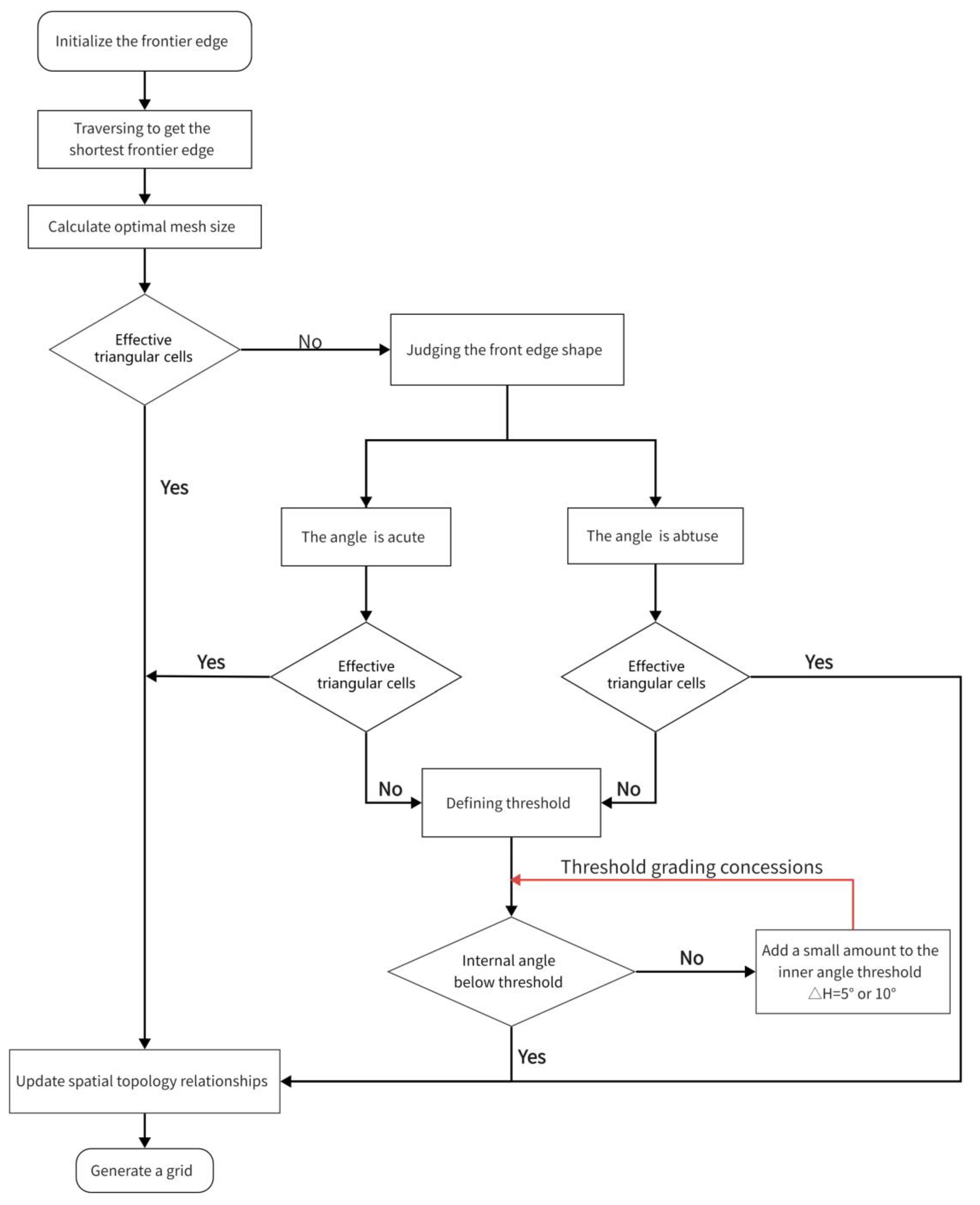
The optimization and update of the front edge promotion algorithm mainly involves three aspects, namely, the deletion of the original front edge segment, the update of the topological relationship between the new front edge segment, and the front edge segment. The alternative digital tree (ADT) data structure proposed by Bonet et al. was used for data storage to improve the efficiency of the frontier algorithm update [32]. On the basis of the classification of the above complex front edge patterns and the corresponding mesh element construction strategy, the adaptive mesh generation algorithm is applied in Figure 2:

The specific steps of the algorithm are the following steps:

Step 1: Build a background mesh of unit dimensions, discretize the boundaries of the area, and initialize the front edges.

Step 2: Traverse to find the shortest length segment among all front edge edges and calculate the optimal mesh cell size at the middle point of this segment and the position of the mesh node to be selected. The optimal mesh element size [33,34] is calculated as:

$$\mathsf{\alpha }\left(ABC\right)=4\sqrt{3}\frac{S}{l_a{}^2+l_b{}^2+l_c{}^2}$$

(1)

$$\mu =\frac{s}{\rho }\left(2-\frac{s}{\rho }\right)a=\frac{h}{H}\left(2-\frac{h}{H}\right)\frac{2\sqrt{3}dh}{2h^2+1.5d^2}$$

(2)

where $S$ represents the area of the unit. $l_a$, $l_b$, and $l_c$ represent the lengths of the three sides of the unit, respectively, $s$ represents the actual size of the unit, $\rho$ represents the size obtained from the background mesh at the midpoint of the shortest line segment, and $a$ represents the form quality.

Table 1. Morphological mass $a$ of different elements and their corresponding geometric morphological characteristics of triangular elements.

Unit form Mass $a$	1.0	0.98	0.72	0.45
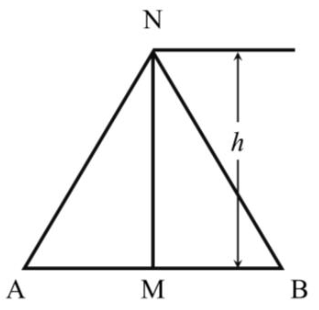
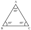
Unit geometry form

shows the geometry of the corresponding $\Delta ABC$. The value range of the mass of the $a$ pattern is $\left(0,1\right)$. When the mass of the $a$ form approaches 1, a closer distance between the geometric form of $\Delta ABC$ and the regular triangle corresponds to a higher mass of this element form. $d_{ab}$ represents the length $AB$ of the line segment in $\Delta ABC$, $h$ represents the height of unit $\Delta ABC$, $H=\sqrt{3}\rho /2$, and the $\mu$ coefficient represents the expected element size of the unit and the element morphological quality of $d_{ab}$ at the same time, as shown in Figure 3.

To calculate the optimal size of unit $\Delta ABC$, let $g=h/d_{ab}$, $k=H/d_{ab}$, and calculate the $\mu \left(g\right)$ coefficient from Equation (2) as follows:

$$\mu \left(g\right)=\frac{\sqrt{3}}{k}\left(2-\frac{g}{k}\right)\frac{2g^2}{2g^2+1.5}$$

(3)

In order for the $\mu \left(g\right)$ coefficient to take the maximum value, let $\frac{d\mu }{dg}=0:$

$$F\left(g\right)=g^3+2.25g-3k$$

(4)

By taking $g_0=0, F\left(g_0\right)=-3k$, based on Newton’s iterative method, the following can be obtained:

$$g_1=g_0-\frac{F\left(g_0\right)}{F^{\prime }\left(g_0\right)}=\frac{3k}{2.25}$$

(5)

$$g_{i+1}=g_i-\frac{F\left(g_i\right)}{F^{\prime }\left(g_i\right)}=\frac{2g_i{}^3+3k}{3g_i{}^2+2.25}\hspace{1em}\left(i=0,1,2,\dots \right)$$

(6)

After repeated iterations of the above equations, an approximation of $g$ can be obtained; that is, the actual size of the element $h_0=g\ast d_{ab}$, where $h_0$ represents the optimal size of the mesh element to build, and the cell is built based on the $h_0$ dimension. In this way, the cell achieves the best balance between self-adaptation and cell shape quality.

Step 3: If the cell formed by the mesh node to be selected is invalid, then $h_0=0.8\ast h_0$. The position of the mesh node to be selected is then solved iteratively, which needs to meet $h_0>\left|AB\right|/2$. Afterwards, determine whether this mesh node can be built into a valid unit. If a valid cell can be formed, then Step 8 is executed directly. Otherwise, Step 4 is executed.

Step 4: If the included angle between the selected line segment and the adjacent front edge line segment is acute and a valid cell can be generated by connecting the non-common points of the included angle, then execute Step 8. If a valid cell cannot be formed, then execute Step 5.

Step 5: If the included angle between the selected line segment and the adjacent front edge line segment is obtuse and if the unit that can be formed by the angle bisector of the obtuse angle is a valid triangular unit, then execute Step 8. Otherwise, execute Step 6.

Step 6: A hierarchical concession strategy based on the threshold is adopted. First, an internal angle threshold is set, and then all the internal angles in the front edge are traversed to screen those internal angles that are below the threshold. If the non-common points trying to connect the included angle can generate a valid element, then the geometry of the front edge will change. If the geometric form of the front edge meets the requirement that the selected line segment and its adjacent front edge segment non-common points form a valid cell, then execute Step 8. Otherwise, execute Step 7.

Step 7: Add a small amount to the threshold value of the included angle, which can be set to 5° or 10° generally, and then return to Step 6.

Step 8: Generate a new mesh cell and update the spatial topological relationship between the front edge and the mesh cell. By determining the number of line segments in the front edge, if the number of line segments is greater than 0, then execute Step 2. If the number of line segments is 0, then the mesh cell generation is completed, and the adaptive mesh generation algorithm is terminated.

3. Mesh Optimization and Smoothing

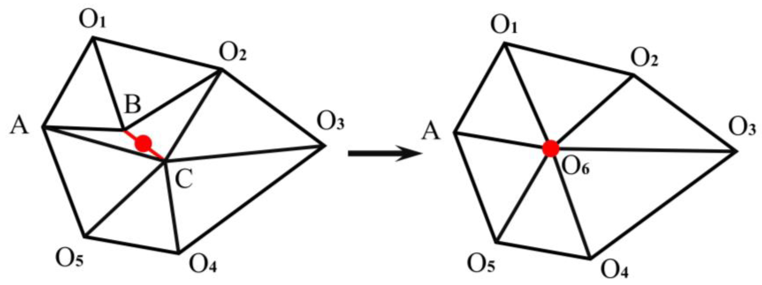
After the adaptive lattice generation, the lattice needs to be smoothed and optimized, and a neighborhood polygon optimization processing strategy is proposed. As shown in Figure 4, the triangular unit $\Delta ABC$ has a poor-quality geometry and should therefore be deleted. At this point, all neighboring $\Delta ABC$ near the shortest side $BC$ of the triangle form the polygon $A{O}_1{O}_2{O}_3{O}_4{O}_5$. A polygon is convex if all of its interior angles are below 180° and if the number of acute angles is less than or equal to 3. $\Delta ABC$ is assumed to satisfy the neighborhood polygon optimality treatment condition. On the basis of the optimal neighborhood, all triangular elements adjacent to the element to be optimized are eliminated, and the midpoint position of the shortest side of the element is obtained and connected to the vertices of each polygon. Therefore, a new triangular element is generated, and the smoothing and optimization of the mesh element are realized.

If non-convex, then this neighboring polygon needs to be “convexized” as shown in Figure 5. Screen the first inner angle that exceeds 180°, derive its adjacent front edge segments, and record them as $L_i$ and $L_j$, respectively. Afterwards, connect the non-common nodes of frontier segments $L_i$, $L_j$ to generate a new frontier edge $L_n$. At this time, $L_n$ can be used to replace $L_i$ and $L_j$, and then the spatial topology of each side of the neighboring polygon can be updated. Afterwards, determine whether the neighboring polygon is convex. If it is convex, then complete the “convexification” [35,36] process; otherwise, continue repeating the above steps until the neighboring polygon becomes convex.

Optimization based on neighborhood polygons can be used to obtain a smoother mesh by adjusting the positions of the mesh nodes, which can generally be carried out by using Laplacian smoothing [37], which can be expressed as:

$$X_i^p=\frac{1}{n}{\displaystyle \sum }_{j=1}^{n_i}{X}_j$$

(7)

where $X_i^p$ represents the adjusted position of the mesh node $i$, and $X_j$ represents the set of coordinates of the $n_i$ points adjacent to point $i$. Mesh smoothing is achieved by adjusting each point to the center of mass of the polygon formed by its neighboring nodes, and the quality of the mesh usually converges to a stable value after two to five iterations.

4. Results and Discussion

4.1. Algorithm and Algorithm Efficiency Analysis

Set the total number of initial front edge segments included in the background mesh boundary to $N_b$ and the total number of cells in the background mesh to $N{E}_b$. Based on the optimization and update forward edge advancing algorithm given above, each time a new mesh cell is generated, the front edge segments and the traversal of all front edge searches need to be cross checked. The algorithm time complexity in this step is $O\left(N_b\right)$. When calculating the mesh cell size, the cell of the background mesh in which the node to be selected is located should be determined. The algorithm time complexity in this step is $O\left(N{E}_b\right)$.

Set the total number of cells in the final mesh to $N_e$. Given that each cell has to obtain the size information from the background mesh, there exists $O\left(N_e\right)=O\left(N{E}_b\right)>O\left(N_b\right).$ Therefore, the time complexity of all mesh adaptive generation algorithms is $O\left(N_e{}^2\right)$. All background mesh information is stored based on the ADT data structure. At this time, the time complexity of the retrieval algorithm to obtain the background mesh size is $O\left(lo{g}_2\left( N{E}_b\right)\right)$, and given that $O\left(lo{g}_2\left( N{E}_b\right)\right)<O\left(N_b\right)$, the time complexity of all mesh adaptive generation algorithms is $O\left(N_e\times N_b\right)$.

To verify the accuracy and applicability of the edge advancing algorithm before optimization, a simulation system of finite element adaptive mesh construction is designed using C++ language based on the OpenGL visualization engine. The running environment parameters of the system experiment are as follows: Windows 10; 8 G memory; Intel (R) Core (TM) i7-6700H CPU @ 3.40GHz processor. The main functions include initialization and discrete simulation boundary, setting the background mesh size, and generating, optimizing, and smoothing TIN. The overall quality of the mesh is used as the basis for measuring the quality of the adaptive mesh generation. The overall quality of the mesh is calculated as

$$Q\left(mesh\right)=\frac{{\sum }_{i=1}^{N_e}{\alpha }_i}{N_e}$$

(8)

where $Q\left(mesh\right)$ represents the overall quality of the mesh, $N_e$ represents the total number of cells contained in this mesh, and ${\alpha }_i$ represents the morphological mass of the first unit, which can be calculated using Equation (1).

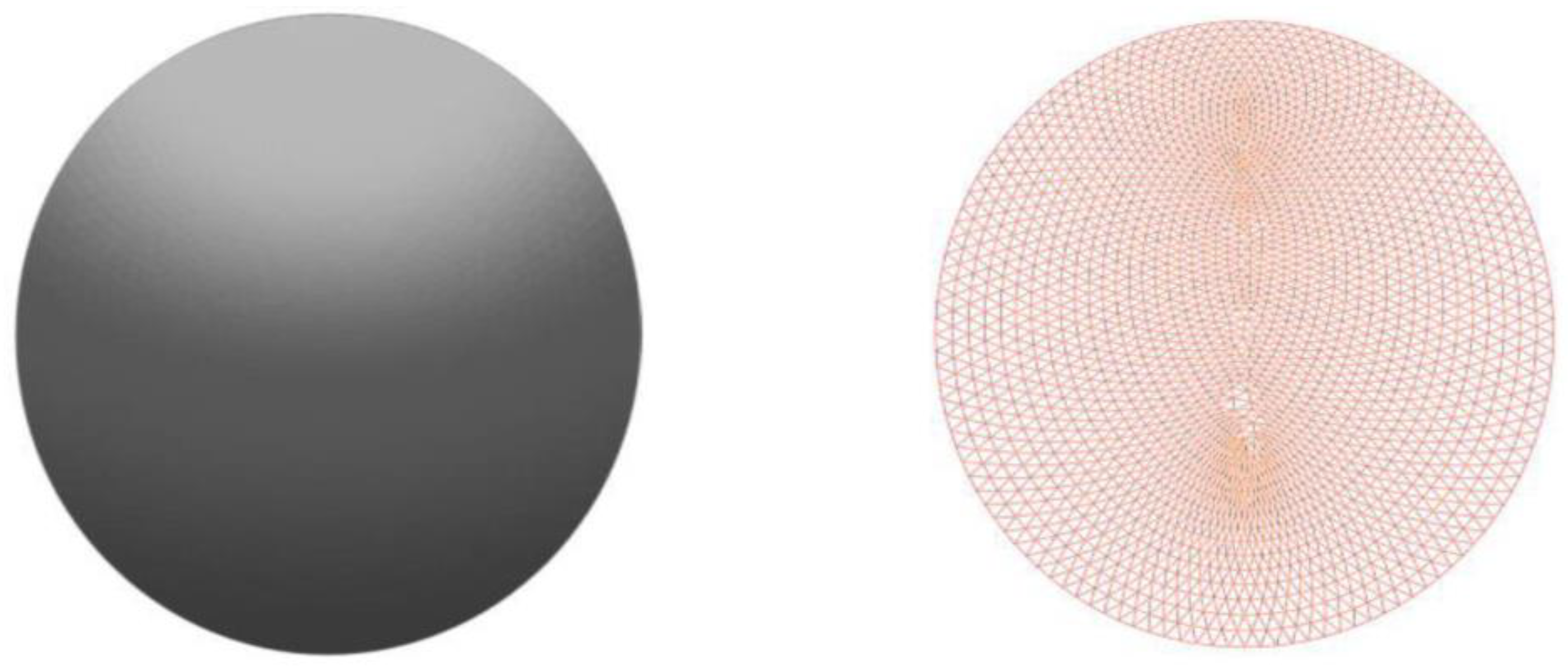
Two examples, a circle and an irregular polygon, were selected to generate the background mesh and adaptive mesh, respectively. As shown in Figure 6 and Figure 7, the size of the adaptive mesh unit was obtained from the background mesh in the left figure. The color shading degree represents the expected size of the mesh unit at this location. A brighter color indicates a smaller expected size, whereas a darker color indicates a larger expected size. The figure on the right presents the adaptive triangle network that is constructed according to the background mesh. The mesh generation results show that the adaptive mesh and background mesh have good fitting ability. The background mesh can be used to flexibly adjust the adaptation of the mesh, and mesh units with a smooth transition and high overall quality can be obtained.

4.2. Execution Time Analysis

Table 2. Time consumption of adaptive mesh unit generation and mesh quality before and after optimization.

Example	Total Number of Units	Overall Time Consumption (s)	Generating Mesh Time Consuming (s)	Optimizing Mesh Time Consuming (s)	Smoothing Mesh Time Consuming (s)	Before Optimization Mesh Quality	After Optimization Mesh Quality
Example 1	3898	15.225	0.415	12.458	0.352	0.891	0.920
Example 2	4042	28.414	0.504	27.546	0.364	0.884	0.918

shows the time spent on mesh generation, mesh optimization, and mesh smoothing for the two examples. The algorithm took the longest time to run the mesh optimization step. For nearly 4000 units of the mesh, the mesh optimization took more than 15 s, and the algorithm efficiency was low. By contrast, the mesh generation and smoothing steps only took less than a second and are therefore more efficient.

Mesh optimization takes the longest time to run as it requires multiple global mesh judgments during the implementation of neighborhood polygon optimization operations. Therefore, after mesh optimization, the overall quality of the mesh elements had only been improved to a limited extent. Given the good quality of the mesh generated based on the AFT mesh generation algorithm, the mesh optimization operation is often applied in local areas during practical applications. Meanwhile, for mesh in the global scope, the mesh optimization module is generally not called for.

4.3. Mesh Quality Analysis

Table 3. Quality comparison of adaptive mesh generated by this algorithm and the traditional algorithm.

Example	Programs	$\mathit{T}\left(\mathit{s}\right)$	$\mathit{N}\mathit{e}$	$\mathit{Q}$	${\mathit{Q}}_{\mathit{a}}$	${\mathit{Q}}_{\mathit{z}}$	$\mathit{P}\left({\mathit{Q}}_{\mathit{e}}<0.4\right)$	$\mathit{P}\left(0.4<{\mathit{Q}}_{\mathit{e}}<0.9\right)$	$\mathit{P}\left({\mathit{Q}}_{\mathit{e}}>0.9\right)$
Example 1	R-TIN Algorithm	0.415	4676	0.89	1.00	0.28	2.59%	26.21%	71.20%
	Traditional Algorithm	0.840	4636	0.83	1.00	0.02	2.14%	35.06%	62.80%
Example 2	R-TIN Algorithm	0.504	4042	0.89	1.00	0.12	4.74%	24.36%	70.90%
	Traditional Algorithm	0.915	4021	0.83	1.00	0.04	4.35%	34.20%	61.50%

compares the quality of the adaptive meshes generated by the optimized AFT algorithm and the traditional AFT algorithm. The average quality of the mesh constructed by the optimized AFT algorithm could reach more than 0.9, and the total number of cells with a form quality of below 0.4 accounted for less than 5% of the total. Compared with the traditional AFT algorithm, the optimized AFT algorithm took less time and could effectively improve the overall quality of mesh cells.

$T$ represents the calculation time, $N_e$ stands for the total number of units, $Q$ represents the overall quality of the mesh, $Q_a$ represents the element mass of the optimal form, $Q_z$ represents the element mass of the worst form, $P$ represents the percentage of the element whose mass reaches a certain range, and $Q_e$ represents the morphological mass of a single cell. The above results show that the morphological quality of the mesh elements generated by the proposed optimized AFT algorithm was relatively stable, and most of these elements were distributed in the $\left(0.9,1\right)$ interval. In addition, a small number of cells in the mesh had a mass of below 0.4 because the AFT algorithm had front edge intersections during the calculation. However, in the range where the boundary shape was regular and the size change was stable, the AFT algorithm had fewer front edge intersections during the calculation, thereby reducing the number of elements with a mass of below 0.4.

In sum, the adaptive mesh generated by the proposed optimized AFT algorithm had better quality, transition, and adaptability compared with that generated by the traditional AFT algorithm. The optimal node position and element shape were then dynamically calculated based on the mapping relationship between the set effective size and the size control data. The traditional AFT algorithm was then improved in terms of its operation efficiency and robustness. The adaptive triangulation network could support the spatial variation expression of the characteristic parameters of the aquifer medium in the groundwater system at the horizontal level.

5. Application of Algorithms in 3D Geological Modeling

The TIN model is the most commonly used surface modeling model based on discrete sampling points. Given the complexity of geological conditions and the limitations of a single model, building a 3D model that can eventually meet all geological conditions becomes a challenge. Therefore, hybrid models have recently attracted much research attention; for example, using the Tetrahedral Network (TEN) [38] as the basic modeling body element, and the hybrid model [39,40] TGT of the geological body based on TIN-GTP-TEN. Using borehole data to construct a triangular network TIN on the surface of the geological body, the geological body is decomposed into the generalized trigonal model (GTP) [41,42,43] via vertical conjoining, and then the GTP is dissected into TEN. This method reduces the difficulty of constructing a geological body model and avoids the other body element models of cutting and self-decomposition, which are generally difficult and tedious, thereby reducing the computational difficulty.

Following the previous research findings of our team, an optimized adaptive triangulation algorithm (R-TIN) was proposed based on TIN, and an automatic identification algorithm of the front edge shape type was introduced. The designed optimal cell construction strategy module could be quickly retrieved and called to generate an adaptive mesh. Take Nantong City in the eastern coastal region of China as an example, in which 160 engineering geological boreholes were deployed. The boreholes and engineering geological layer information in this area was relatively detailed and could reflect the spatial distribution patterns and lithological characteristics of its stratigraphy. Using the original data from the engineering geological exploration and the actual drilling, the team initially extracted information on controlled discrete points with high accuracy. With these data as constraints, virtual drilling was constructed and combined. Afterwards, the area discrete mesh data were established using the advancing front AFT algorithm, which integrates the automatic discrimination mechanism of the complex morphological types of the optimized front edge. The adaptive and dynamic generation of R-TIN was eventually carried out, and the stratum boundary was generated by combining with the engineering geological stratum layering boundary. A 3D geological engineering modeling was eventually realized based on the RTGT mixed model.

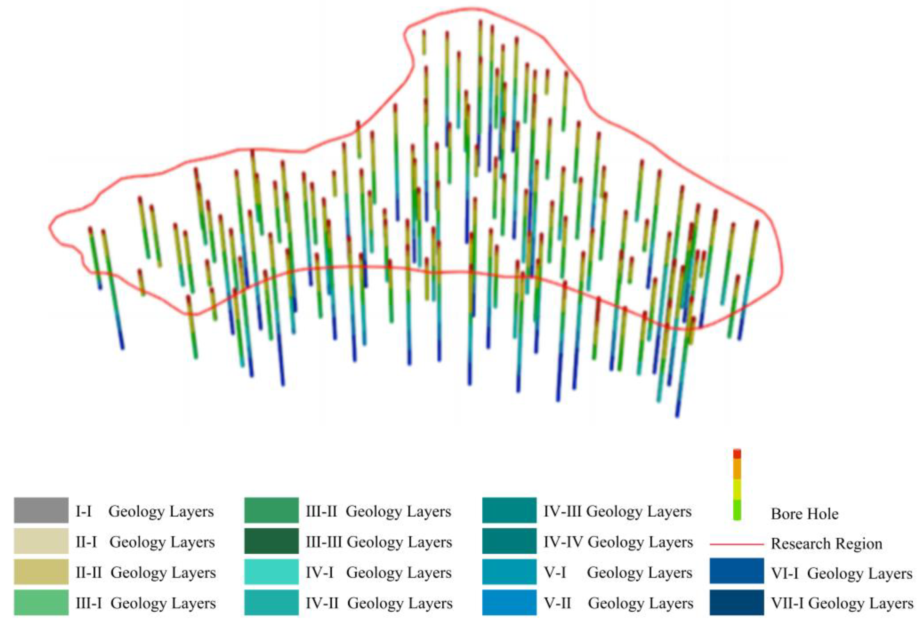
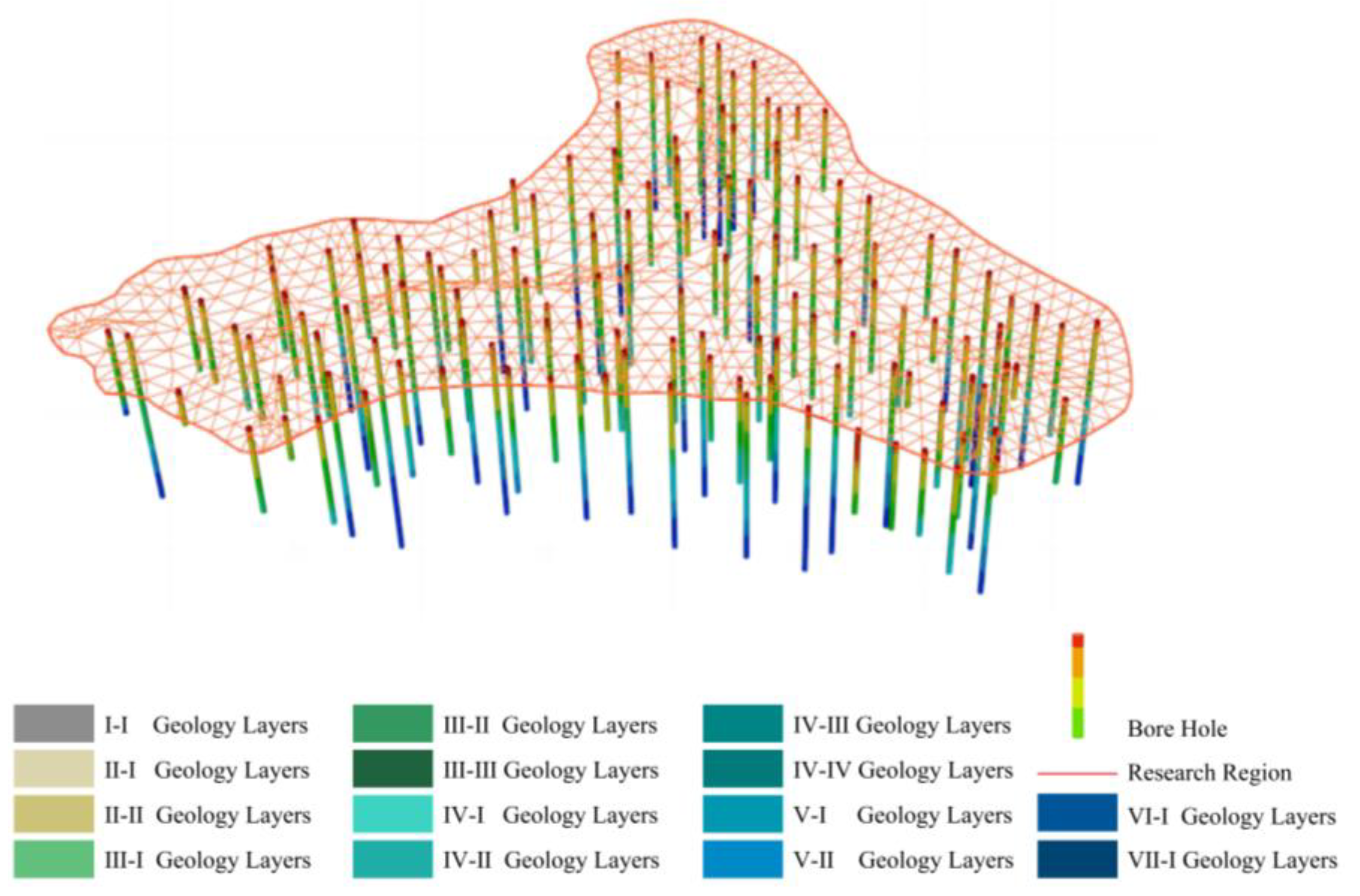
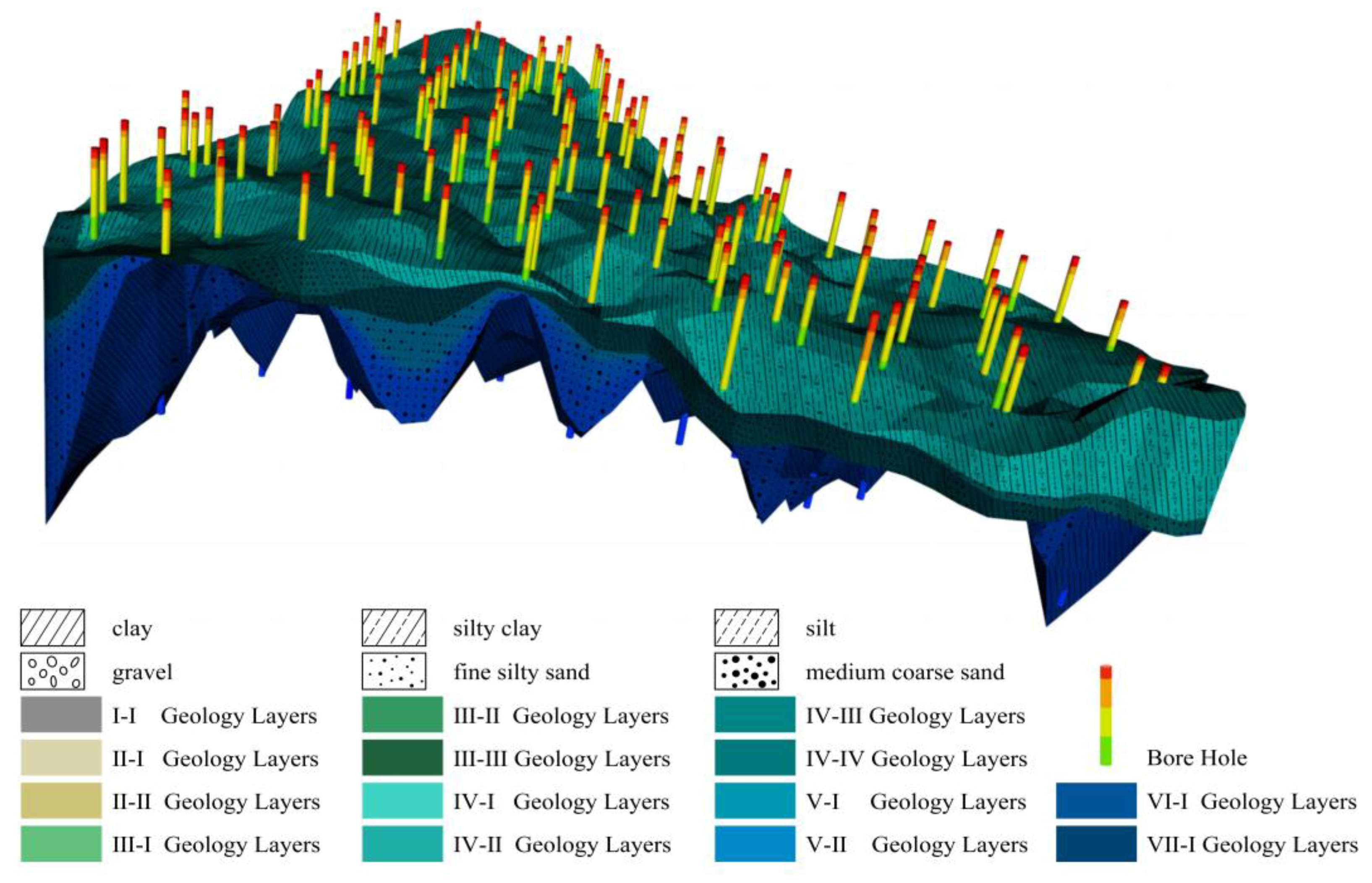
Engineering geological drilling is the main data source for 3D engineering geological modeling, whose 3D drilling model [44,45] is represented by segmented cylinders. Each segment of the cylinder corresponds to different strata. The height of each segment is determined by the thickness of the strata and distinguished by different colors. The visualization results of the engineering geological drilling and the boundary model of the study area are shown in Figure 8. Different geological layers are shaded in different colors. The regional adaptive dynamic TIN model is shown in Figure 9.

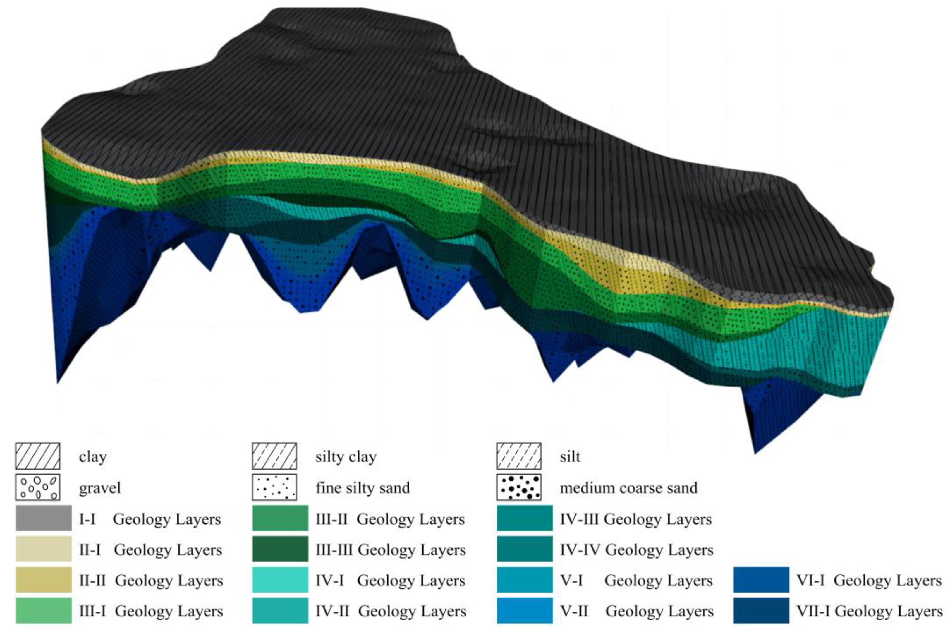
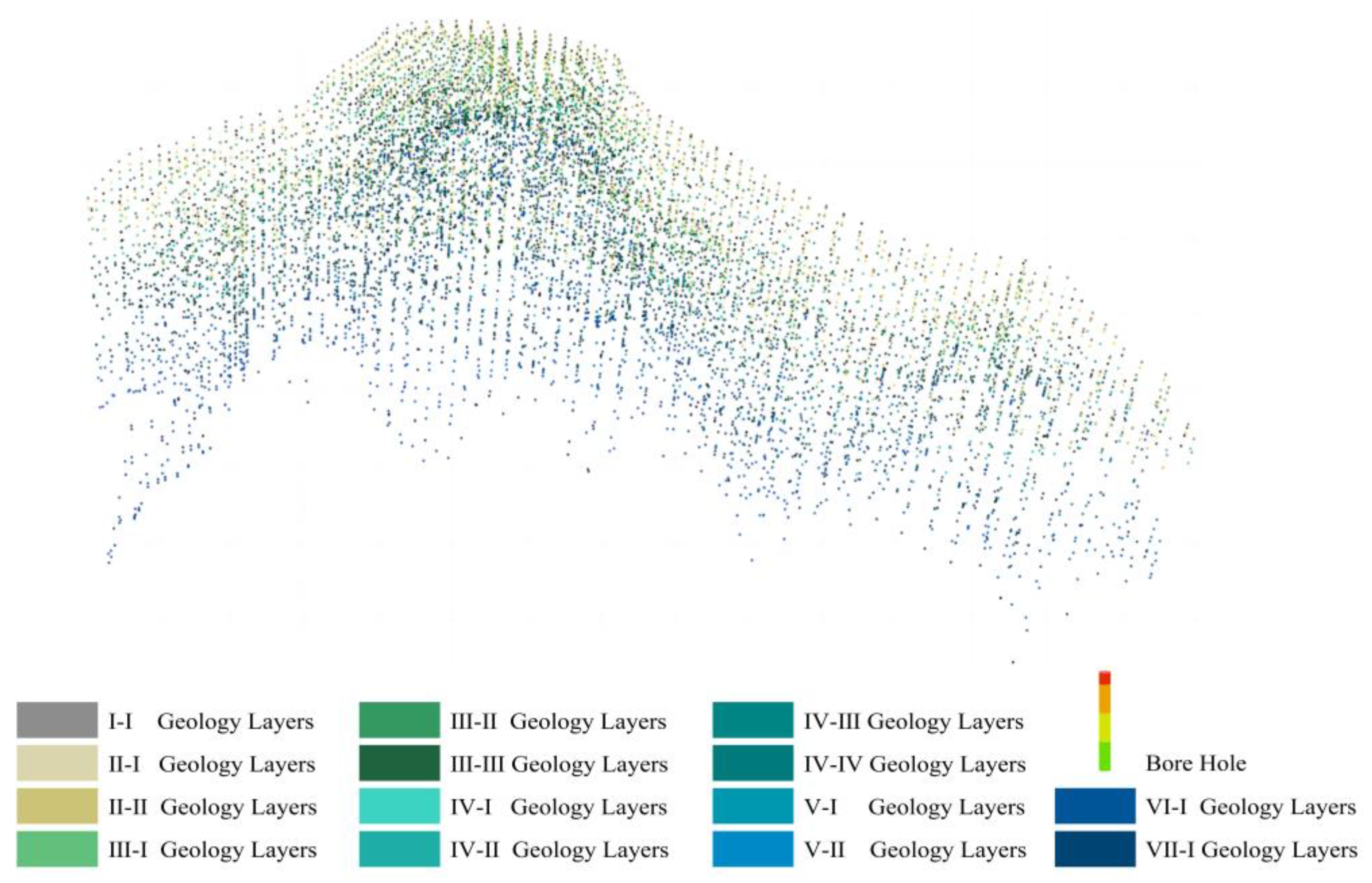
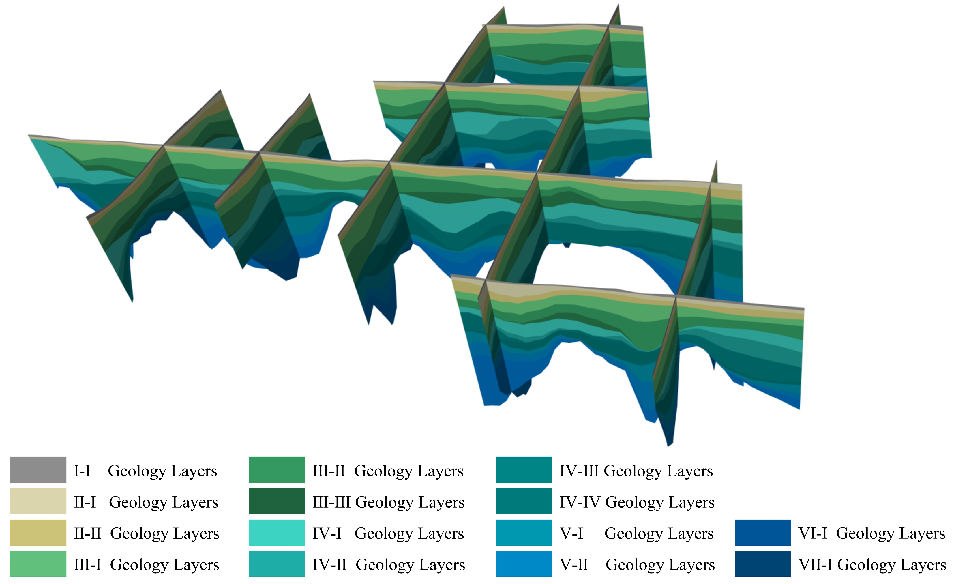
On the basis of the drill hole data retrieved from the study area, the R-TIN-GT hybrid model was used to establish the regional 3D engineering geological model, as shown in Figure 10. The lithology of the strata was then divided into different strata as indicated by different colors and symbols, and the thickness of these layers was determined by the actual thickness of the strata. Figure 11 shows the engineering geological point cloud model, whereas Figure 12 shows the 3D model of engineering geology and the modeling drilling hole fusion model. The spatial distribution characteristics of each engineering geological layer can be viewed by extracting its strata. Figure 13 shows the structural fence of engineering geological layers. After profiling the 3D geological model, a uniform fence surface was established to comprehensively observe the stratigraphic spreading of the entire study area from a spatial scale. Therefore, the fence surface shear model can be used to obtain a 3D perspective profile of the engineering geological model.

The R-TIN model mesh element generated by the optimized adaptive front advancing algorithm had a good quality and an excellent boundary fitting effect and considered the quality and robustness of the triangle element. Moreover, the GTP model based on R-TIN had high flexibility, few restrictions on the spatial unit shape, a diversified expression, and strong applicability. Therefore, building a 3D geological model based on the R-TIN-GT mixed model not only effectively improves the quality and efficiency of the surface TIN model, but also improves the accuracy and visualization effect of the overall geological model.

6. Conclusions

This study proposed an optimized adaptive triangulation dynamic generation algorithm called R-TIN. Taking engineering geology as an example, based on the generalized triangular prism GTP model and the tetrahedron TEN model, a hybrid 3D engineering geological modeling method called R-TIN-GT was introduced. The results showed that the quality of the self-adaptive dynamic generation of TIN could be improved by using the advancing front algorithm, which integrates the automatic discrimination mechanism of the complex morphology of the front edge. More than 70% had a quality exceeding 0.9 overall, and the overall quality and efficiency of the mesh units were improved to a certain extent. The discrete mesh generated by the optimized advancing front and adaptive dynamic generation algorithms had high quality, and the consumed time was reduced to a certain extent. Given its smooth transition and strong adaptability, the proposed model could well support the construction of an irregular triangular network of the engineering geological surface. The feasibility and effectiveness of the modeling method based on the optimized triangulation algorithm could provide intuitive 3D geological information.

Although this research has made some improvements to the traditional front advancing method, a perfect solution to the poor quality of the front edge intersection elements is yet to be found. How to further improve the efficiency of mesh optimization and reduce the “intersection” effect of the front edge also warrants examination. The algorithm and construction of an accurate 3D engineering geological model also need further improvements to reflect 3D geological information and geological phenomena, such as faults and folds.

References

1. Zhu, M.; Scott, M.H. A PFEM Background Mesh for Simulating Fluid and Frame Structure Interaction. J. Struct. Eng. 2022, 148, 04022051. [Google Scholar] [CrossRef]
2. Luo, T.X.; Yuan, P.; Zhu, S. Automatic modelling of urban subsurface with ground-penetrating radar using multi-agent classification method. Geo-Spat. Inf. Sci. 2022, 25, 588–599. [Google Scholar] [CrossRef]
3. Zhang, M.; Xie, Z.; He, L. Does the scarcity of urban space resources make the quality of underground space planning more sustainable? A case study of 40 urban underground space master plans in China. Front. Environ. Sci. 2022, 10, 2162. [Google Scholar] [CrossRef]
4. Guo, J.; Wang, X.; Wang, J.; Dai, X.; Wu, L.; Li, C.; Li, F.; Liu, S.; Jessell, M.W. Three-dimensional geological modeling and spatial analysis from geotechnical borehole data using an implicit surface and marching tetrahedra algorithm. Eng. Geol. 2021, 284, 106047. [Google Scholar] [CrossRef]
5. Hao, M.; Li, M.; Zhang, J.; Liu, Y.; Huang, C.; Zhou, F. Research on 3D geological modeling method based on multiple constraints A case study of Huaying Mountain Kangyangju in Guang’an City. Earth Sci. Inform. 2021, 14, 291–297. [Google Scholar] [CrossRef]
6. Wang, Y.; Liang, X.; Flener, C.; Kukko, A.; Kaartinen, H.; Kurkela, M.; Vaaja, M.; Hyyppa, H.; Alho, P. 3D Modeling of Coarse Fluvial Sediments Based on Mobile Laser Scanning Data. Remote Sens. 2013, 5, 4571–4592. [Google Scholar] [CrossRef]
7. Costantino, D.; Vozza, G.; Alfio, V.S.; Pepe, M. Strategies for 3D Modelling of Buildings from Airborne Laser Scanner and Photogrammetric Data Based on Free-Form and Model-Driven Methods: The Case Study of the Old Town Centre of Bordeaux (France). Appl. Sci. 2021, 11, 10993. [Google Scholar] [CrossRef]
8. Zhu, L.; Zhang, C.; Li, M.; Pan, X.; Sun, J. Building 3D solid models of sedimentary stratigraphic systems from borehole data: An automatic method and case studies. Eng. Geol. 2012, 127, 1–13. [Google Scholar] [CrossRef]
9. Robert, M.; Carmen, J.; Fritz, Z. A visual LISP program for voxelizing AutoCAD solid models. Comput. Geosci. 2015, 74, 110–120. [Google Scholar] [CrossRef]
10. Spirou-Sioula, K.; Ioannidis, C.; Potsiou, C. Technical aspects for 3D hybrid cadastral model. Surv. Rev. 2013, 45, 419–427. [Google Scholar] [CrossRef]
11. Martinez, J.L.; Raiber, M.; Cendon, D.I. Using 3D geological modelling and geochemical mixing models to characterise alluvial aquifer recharge sources in the upper Condamine River catchment, Queensland, Australia. Sci. Total Environ. 2017, 574, 1–18. [Google Scholar] [CrossRef] [PubMed]
12. Zhu, J.; Wang, X.; Chen, M.; Wu, P.; Kim, M.J. Integration of BIM and GIS: IFC geometry transformation to shapefile using enhanced open-source approach. Autom. Constr. 2019, 106, 102859. [Google Scholar] [CrossRef]
13. Luo, Y.-T.; Du, H.; Yan, Y.-M. MeshCNN-based BREP to CSG conversion algorithm for 3D CAD models and its application. Nucl. Sci. Tech. 2022, 33, 74. [Google Scholar] [CrossRef]
14. Li, C.; Li, F.; Guo, J.; Liu, C.; Chen, F.; Liu, Y. 3D geological map modeling technology based on a geological route and geological object wireframe model. Acta Geol. Sin. 2019, 92, 231. [Google Scholar]
15. Cheng, X. Algorithm of CAD Surface Generation for Complex Pipe Model in Industry 4.0 Background. Comput. Intell. Neurosci. 2022, 2022, 7062052. [Google Scholar] [CrossRef]
16. Quan, Y.; Song, J.; Guo, X.; Miao, Q.; Yang, Y. Filtering LiDAR data based on adjacent triangle of triangulated irregular network. Multimed. Tools Appl. 2017, 76, 11051–11063. [Google Scholar] [CrossRef]
17. Zhao, Z.; Cheng, C.; Jin, X.; Liu, L.; Yan, L. A MILP model for hydro unit commitment with irregular vibration zones based on the constrained Delaunay triangulation method. Int. J. Electr. Power Energy Syst. 2020, 123, 106241. [Google Scholar] [CrossRef]
18. Hu, G.; Wang, C.; Li, S.; Dai, W.; Xiong, L.; Tang, G.; Strobl, J. Using vertices of a triangular irregular network to calculate slope and aspect. Int. J. Geogr. Inf. Sci. 2021, 36, 383–405. [Google Scholar] [CrossRef]
19. Zhao, L.; Li, G.; Yao, X.; Ma, Y.; Cao, Q. An optimized hexagonal quadtree encoding and operation scheme for icosahedral hexagonal discrete global grid systems. Int. J. Digit. Earth 2022, 15, 975–1000. [Google Scholar] [CrossRef]
20. Liang, X.; Ben, J.; Wang, R.; Liang, Q.; Huang, X.; Ding, J. Construction of rhombic triacontahedron discrete global grid systems. Int. J. Digit. Earth 2022, 15, 1760–1783. [Google Scholar] [CrossRef]
21. Hu, G.; Xiong, L.; Lu, S.; Chen, J.; Li, S.; Tang, G.; Strobl, J. Mathematical vector framework for gravity-specific land surface curvatures calculation from triangulated irregular networks. GISci. Remote Sens. 2022, 59, 590–608. [Google Scholar] [CrossRef]
22. Wang, S.; Gao, Z.; Wang, Z.; Wu, X.; An, Y.; Ren, X.; He, M.; Wang, W.; Liu, J. Hydrodynamic characteristics of groundwater aquifer system under recharge and discharge conditions. Arab. J. Geosci. 2020, 13, 859. [Google Scholar] [CrossRef]
23. Vu, M.T.; Jardani, A.; Massei, N.; Fournier, M. Reconstruction of missing groundwater level data by using Long Short-Term Memory (LSTM) deep neural network. J. Hydrol. 2021, 597, 125776. [Google Scholar] [CrossRef]
24. Sastry, S.P. A 2D advancing-front Delaunay mesh refinement algorithm. Comput. Geom. 2021, 97, 101772. [Google Scholar] [CrossRef] [PubMed]
25. Zhou, Q.; Wang, Q.; Yu, Z. SAFT: Shotgun advancing front technique for massively parallel mesh generation on graphics processing unit. Int. J. Numer. Methods Eng. 2022, 123, 4391–4406. [Google Scholar] [CrossRef]
26. Lu, P.; Wang, N.; Chang, X.; Zhang, L.; Wu, Y.; Zhang, H. An Automatic Isotropic Triangular Grid Generation Technique Based on an Artificial Neural Network and an Advancing Front Method. Math. Probl. Eng. 2022, 2022, 8103813. [Google Scholar] [CrossRef]
27. Meng, L.; Tong, X.; Fan, S.; Cheng, C.; Chen, B.; Yang, W.; Hou, K. A Universal Generating Algorithm of the Polyhedral Discrete Grid Based on Unit Duplication. ISPRS Int. J. Geo-Inf. 2019, 8, 146. [Google Scholar] [CrossRef]
28. Lei, Y.; Tong, X.; Qu, T.; Qiu, C.; Wang, D.; Sun, Y.; Tang, J. A scale-elastic discrete grid structure for voxel-based modeling and management of 3D data. Int. J. Appl. Earth Obs. Geoinf. 2022, 113, 103009. [Google Scholar] [CrossRef]
29. Rangarajan, R.; Kabaria, H.; Lew, A. An algorithm for triangulating smooth three-dimensional domains immersed in universal meshes. Int. J. Numer. Methods Eng. 2019, 117, 84–117. [Google Scholar] [CrossRef]
30. Adamoudis, L.D.; Koini, G.; Nikolos, I.K. Heuristic repairing operators for 3D tetrahedral mesh generation using the advancing-front technique. Adv. Eng. Softw. 2012, 54, 49–62. [Google Scholar] [CrossRef]
31. Ding, H.; Xu, X.; Luo, Y. Generating Free-Form Grid Truss Structures from 3D Scanned Point Clouds. Math. Probl. Eng. 2017, 2017, 5818627. [Google Scholar] [CrossRef]
32. Isailovic, V.; Filipovic, N. An algorithm for finding and adding boundary conditions with the aim of solving the contact problem in computational mechanics. Simul. Model. Pract. Theory 2021, 108, 102247. [Google Scholar] [CrossRef]
33. Liu, Z.; Lv, H.; Li, M.; Li, Z.; Huang, Z. A Novel Self-adaptive Grid-partitioning Noise Optimization Algorithm Based on Differential Privacy. Comput. Sci. Inf. Syst. 2019, 16, 915–938. [Google Scholar] [CrossRef]
34. Letnik, T.; Bozicnik, S.; Spacapan, S.; Mencinger, M. Optimal covering of the equidistant square grid network. Discret. Appl. Math. 2021, 296, 85–89. [Google Scholar] [CrossRef]
35. Nguyen, T.T.; Richard, J.-P.P.; Tawarmalani, M. Convexification techniques for linear complementarity constraints. J. Glob. Optim. 2021, 80, 249–286. [Google Scholar] [CrossRef]
36. Chandra, A.; Tawarmalani, M. Probability estimation via policy restrictions, convexification, and approximate sampling. Math. Program. 2022, 196, 309–345. [Google Scholar] [CrossRef]
37. Khademloo, S. A Multiplicity Result for Quasilinear Problems with Nonlinear Boundary Conditions in Bounded Domains. Int. J. Math. Math. Sci. 2011, 2011, 419341. [Google Scholar] [CrossRef]
38. Zhao, Z.H.; Wang, W.M.; Wang, L.H.; Yan, J.X. Analytical Solution of Interface Effect on the Strength of Combined Model Composed of Different Geologic Bodies. Math. Probl. Eng. 2014, 2014, 549–566. [Google Scholar] [CrossRef]
39. He, L.; Zhang, J.; Chen, S.; Hou, M.; Chen, J. Three-dimensional hydrogeological modeling method and application based on TIN-GTP-TEN. Earth Sci. Inform. 2022, 15, 337–350. [Google Scholar] [CrossRef]
40. Wu, L. Topological relations embodied in a generalized tri-prism (GTP) model for a 3D geoscience modeling system. Comput. Geosci. 2004, 30, 405–418. [Google Scholar] [CrossRef]
41. Sun, L.; Wei, Y.; Cai, H.; Xiao, J.; Yan, J.; Wu, S. Adaptive Interpolation Method for Generalized Triangular Prism (GTP) Geological Model Based on the Geometric Smoothness Rule. Front. Earth Sci. 2022, 10, 254. [Google Scholar] [CrossRef]
42. Shi, C.; Wang, Y. Data-driven construction of Three-dimensional subsurface geological models from limited Site-specific boreholes and prior geological knowledge for underground digital twin. Tunn. Undergr. Space Technol. 2022, 126, 104493. [Google Scholar] [CrossRef]
43. Wu, L.; Shi, W. GTP-based Integral Real-3D Spatial Model for Engineering Excavation GIS. Geo-Spat. Inf. Sci. 2004, 7, 123–128. [Google Scholar] [CrossRef]
44. Kim, H.-S.; Ji, Y. Three-dimensional geotechnical-layer mapping in Seoul using borehole database and deep neural network-based model. Eng. Geol. 2022, 297, 106489. [Google Scholar] [CrossRef]
45. Liu, J.B.; Fang, L.L. Several Topological Indices of Two Kinds of Tetrahedral Networks. J. Math. 2021, 2021, 9800246. [Google Scholar] [CrossRef]
Figure 1. Schematic diagram of front edge morphology classification.
Sustainability 15 07214 g001
Figure 2. Flow chart of adaptive mesh generation algorithm.
Sustainability 15 07214 g002
Figure 3. The optimal mesh cell size h of node N to be selected.
Sustainability 15 07214 g003
Figure 4. Optimization process of long and narrow triangular element.
Sustainability 15 07214 g004
Figure 5. Neighborhood polygon optimization algorithm.
Sustainability 15 07214 g005
Figure 6. Example 1: Background mesh and adaptive mesh of circular area.
Sustainability 15 07214 g006
Figure 7. Example 2: Background mesh and adaptive mesh of irregular polygons.
Sustainability 15 07214 g007
Figure 8. Three-dimensional model of engineering geological borehole.
Sustainability 15 07214 g008
Figure 9. Adaptive dynamic triangulation model.
Sustainability 15 07214 g009
Figure 10. Three-dimensional model of engineering geology.
Sustainability 15 07214 g010
Figure 11. Engineering geological point cloud model.
Sustainability 15 07214 g011
Figure 12. Engineering geology 3D model and modeling drilling fusion model.
Sustainability 15 07214 g012
Figure 13. Fence diagram of engineering geological layer structure.
Sustainability 15 07214 g013