Abstract
Prediction of carbon dioxide (CO2) emissions is a critical step towards a sustainable environment. In any country, increasing the amount of CO2 emissions is an indicator of the increase in environmental pollution. In this regard, the current study applied three powerful and effective artificial intelligence tools, namely, a feed-forward neural network (FFNN), an adaptive network-based fuzzy inference system (ANFIS) and long short-term memory (LSTM), to forecast the yearly amount of CO2 emissions in Saudi Arabia up to the year 2030. The data were collected from the “Our World in Data” website, which offers the measurements of the CO2 emissions from the years 1936 to 2020 for every country on the globe. However, this study is only concerned with the data related to Saudi Arabia. Due to some missing data, this study considered only the measurements in the years from 1954 to 2020. The 67 data samples were divided into 2 subsets for training and testing with the optimal ratio of 70:30, respectively. The effect of different input combinations on prediction accuracy was also studied. The inputs were combined to form six different groups to predict the next value of the CO2 emissions from the past values. The group of inputs that contained the past value in addition to the year as a temporal index was found to be the best one. For all the models, the performance accuracies were assessed using the root mean squared errors (RMSEs) and the coefficient of determination (R2). Every model was trained until the smallest RMSE of the testing data was reached throughout the entire training run. For the FFNN, ANFIS and LSTM, the averages of the RMSEs were 19.78, 20.89505 and 15.42295, respectively, while the averages of the R2 were found to be 0.990985, 0.98875 and 0.9945, respectively. Every model was applied individually to forecast the next value of the CO2 emission. To benefit from the powers of the three artificial intelligence (AI) tools, the final forecasted value was considered the average (ensemble) value of the three models’ outputs. To assess the forecasting accuracy, the ensemble was validated with a new measurement for the year 2021, and the calculated percentage error was found to be 6.8675% with an accuracy of 93.1325%, which implies that the model is highly accurate. Moreover, the resulting forecasting curve of the ensembled models showed that the rate of CO2 emissions in Saudi Arabia is expected to decrease from 9.4976 million tonnes per year based on the period 1954–2020 to 6.1707 million tonnes per year in the period 2020–2030. Therefore, the finding of this work could possibly help the policymakers in Saudi Arabia to take the correct and wise decisions regarding this issue not only for the near future but also for the far future.
1. Introduction
Saudi Arabia is the biggest exporter of fossil fuels in the world. Controlling CO2 emissions will help in improving the quality of life all over the world. Therefore, every country has to keep an eye on the CO2 emissions within its region. To do this, the data have to be recorded from sensors, and a qualitative prediction model has to be built. Higher prediction values from this model are alarm signs for expected harmful situations that could inform and help the authorities to take suitable actions.
Despite the fact that the increase in CO2 emissions is harmful to human beings and the environment, an adequate amount of CO2 is an essential requirement for plants and agriculture. According to records, the United Nations announced in the COP27 conference that was held in Sharm Elsheikh, Egypt in November 2022 that CO2 emissions have increased by 1% in 2022 to reach 37.5 billion tonnes [1]. This big number is an alarm to the whole world that the global warming problem will continue, and hence, facing it is a must. Moreover, the promises have to be transferred to real actions on the ground [2]. To be on the right track to reducing CO2 emissions, two strategies have to be considered seriously. The first is to decrease the utility of CO2 emission fuels by increasing the use of other alternatives, such as renewable and green energy sources. The energy obtained from photovoltaic (PV) cells is an example of a renewable energy source. In fact, research is growing rapidly in this direction [3,4]. The second is to increase green agricultural areas. Fortunately, Saudi Arabia is currently adopting two routes to positively participate in decreasing the global warming catastrophe. To help authorities in taking the proper decision, a trustable forecasting tool is required.
The need for data forecasting can be encountered in many engineering applications. Therefore, it obtained great interest from many researchers of different disciplines and directions. To build a forecasting model, there are many tools and techniques to do so. However, building a robust model that can correctly predict future values from past values is a challenging task. In this regard, artificial intelligence (AI) and machine learning (ML) techniques occupy a substantial and competitive position among other tools. They are considered the best-nominated approaches that can perfectly handle data modelling and forecasting tasks [5,6,7,8,9].
The applications of artificial intelligence (AI) and deep learning (DL) tools are growing from day to day. These applications can be categorized into two main fields: classification and prediction. The applications of classifying tools include the fingerprint classifier, voice recognition, image, etc. However, from the prediction tool perspective, applications might include modelling and forecasting of time-series data, traffic, stock, weather, etc. The reliability of a predicting model comes from the appropriate selection of the model’s type, and then a successful training phase is implemented. There are many AI techniques to be used as predictors, such as artificial neural networks (ANNs) [10], adaptive network-based fuzzy inference systems (ANFISs) [11], long short-term memory (LSTM) [12], regression support vector machines (RSVMs) [13], autoregressive integrated moving averages (ARIMAs) [14], etc.
Similarly, AI techniques can be applied to forecast CO2 emissions based on the measured time-series data. Vlachas et al. used LSTM as a forecasting model to forecast time-series of a high-dimensional, chaotic system. The results have been compared with those obtained by the Gaussian processes (GPs) and showed that LSTM performed better than the GP [15]. Amarpuri et. al. applied a deep learning hybrid model based on a convolution neural network (CNN) and long short-term memory network (LSTM), namely, (CNN-LSTM), to predict CO2 levels in India in the year 2020. This study aimed to provide an estimated value of the CO2 emissions in India, as the country had an agreement to reduce the carbon dioxide levels to 30–35% of the level in the year 2005 according to the Paris Agreement [16]. Kumari and Singh used three statistical models, two linear regression models and a deep learning model to predict CO2 emissions in India for the next ten years based on the data from 1980 to 2019 [14]. The statistical models included the autoregressive integrated moving average (ARIMA) model, the seasonal autoregressive integrated moving average with exogenous factors (SARIMAX) model, and the Holt–Winters model. The machine learning models included linear regression and random forest techniques, while the deep learning-based model included long short-term memory (LSTM). They concluded that LSTM outperformed the other five models, which produced an RMSE value of 60.635. Meng and Noman applied four machine learning (ML) SARIMA models, namely, SARIMAX, to predict total CO2 emissions, taking into account the effect of COVID-19 pandemic circumstances in the reduction of the emission value [17]. The study included a comparison between the four prediction models to suggest the effective one based on the lowest value of mean absolute percentage error (MAPE). The authors considered the forecasting periods as near future prediction, future prediction and far future prediction for the years 2022 to 2027, 2022 to 2054 and 2022 to 2072, respectively. They showed that the post-COVID-19 model forecasts CO2 emission in a reasonable behaviour. Birjandi et. al. applied an artificial neural network (ANN) model of eleven neurons in the hidden layer with two different activation functions, normalized RBF and tansig, to predict CO2 in four Southeastern countries: Malaysia, Indonesia, Singapore and Vietnam [18]. They concluded that the ANN model with the normalized RBF produced the highest correlation value with the measured data.
Researchers are promoted to apply AI techniques in the forecasting of CO2 emissions applications. Examples of reputative AI tools are the FFNN, ANFIS and LSTM. Many recent studies used the FFNN [19,20], ANFIS [21,22] and LSTM [14,23,24] techniques to build a forecasting model of CO2 emissions. For the FFNN modelling approach, Mutascu used the single-layer, 20-neuron feed-forward artificial neural network approach to predict CO2 emissions in the United States of America [25]. The model was built based on the annual data collected during the years ranging from 1984 to 2020. The simulation results showed that the forecasting accuracy was 92.42%, and the forecasting error percentage was 7.58%. The RMSE and the R2 were used as the statistical assessment of the modelling accuracy. Moreover, Wang et. al. combined several machine learning tools in a hybrid procedure to forecast CO2 emissions in China [26]. They applied four two-stage procedures. Support vector regression (SVR) with an ANN was one of the used procedures. Regarding the ANFIS modelling tool, Cansiz et. al. applied some AI techniques that included an ANN and ANFIS to predict the CO2 emissions from the transportation sector [21]. Their results showed that the ANN model was the best. For the LSTM technique, Kumari and Singh conducted a comparison study between some ML tools, including LSTM, to predict CO2 emissions in India [14]. They concluded that the LSTM model was the best to predict CO2 emissions, as it produced the lowest RMSE of 60.635 among the other techniques.
Particularly, some researchers applied several AI tools to forecast the CO2 emissions in Saudi Arabia. Hamieh et. al. conducted a study to quantify the CO2 emissions from industrial facilities in Saudi Arabia [27]. They studied the CO2 emissions from six industrial entities, such as electricity generation, desalination, oil refining, cement, petrochemicals and iron and steel, which are responsible for more than 70% of the country’s total emissions. This was to register the details about the emission source locations, rates and characteristics. Alam and AlArjani compared CO2 emission forecasting in Gulf countries based on an annual basis [28]. They used statistical tools such as autoregressive integrated moving averages (ARIMAs), artificial neural networks (ANNs) and Holt–Winters exponential smoothing (HWES) as the forecasting models. Their conclusion was to use the ANN model for forecasting the CO2 in Gulf countries, as it produced the best results relative to the ARIMA and the HWES models. Alajmi studied the modelling of carbon emissions and electricity generation in SA [29]. This study used a structural time-series model (STSM) and logarithmic mean Divisia index (LMDI) for estimating the long-run elasticities. The results showed that three controlling variables such as gross domestic product (GDP), electricity generation and population are significantly affecting carbon dioxide (CO2) emissions. Furthermore, the findings from utilizing the logarithmic mean division index (LMDI) analysis showed that there was an increase of 1377.56 million tonnes in CO2 emissions from the three controlling factors between 1980 and 2017 in Saudi Arabia. Habadi and Tsokos built a statistical-based time-series model to forecast carbon dioxide in the atmosphere in the Middle East and the atmospheric temperature in Saudi Arabia. The model is of a seasonal autoregressive integrated moving average (seasonal-ARIMA) type, and the data are based on the monthly temperature from 1970–2015 [30]. Althobaiti and Shabri performed a comparison between the nonlinear grey Bernoulli model NGBM (1,1) and the GM (1,1) model for predicting the yearly CO2 emissions in Saudi Arabia from 2017 to 2021 based on the data from 1970 to 2016 [31]. The study concluded that the NGBM (1,1) produced better results based on the mean absolute percentage error (MAPE), which was below 10%. Alkhathlan and Javid studied and analyzed the underlying energy demand trend (UEDT) for the total carbon emissions and carbon emissions from the domestic transport sector in Saudi Arabia using a structural time-series technique [32]. The considered data was in the period from 1971 to 2013. The study demonstrated that there is a positive correlation between the growth in real income and CO2 emissions.
From the aforementioned literature review, it can be noticed that some researchers have been interested in CO2 emissions either in Saudi Arabia or the Middle East area. In the following paragraph, a brief description of each study is presented but from a critical viewpoint.
In [27], the work presents a database for the volumetric concentrations of CO2 emissions from all major stationary industrial sources in Saudi Arabia. However, the paper does not show any modelling or forecasting approach. In [28], the authors developed a comparative study between three prediction models, namely, ARIMA, ANN and Holt–Winters exponential smoothing. They used 55 data samples that represent the recordings during the years 1960:2014. Their goal was to build the best model for forecasting CO2 emissions in the annual range of 2015:2025. The paper showed that the ANN was the best, but the paper does not show the value of the training/testing ratio to assess the model’s reliability. In [29], the authors built a structural time series model (STSM) to study the effect of gross domestic product (GDP), electricity generation and population on CO2 emissions in Saudi Arabia between 1980 and 2017. The paper does not show any data-forecasting strategy. In [30], the authors used a statistical forecasting technique, namely, the autoregressive integrated moving average (ARIMA), to predict the atmospheric CO2 in the entire Middle East between 1996–2015. The forecasting range was applied monthly through only the years 2014:2015. In [31], the study used a statistical method, namely, the nonlinear grey Bernoulli model, to forecast CO2 in Saudi Arabia. The model was built using a dataset in the range of 1970:2016, and the forecasting period represents only the annual range between 2017:2021.
Despite all the abovementioned studies being related to CO2 emissions, none of them has used machine learning or artificial intelligence tools to model CO2 emissions in Saudi Arabia. Moreover, none of them has applied the obtained model to forecast the annual emissions between 2020 to 2030. Almost all of these studies have used statistical methods in their work. Furthermore, all of them have used an entire set of data to build a model. However, in our proposed work, three ensembled machine learning tools, such as FFNN, ANFIS and LSTM, have been used to perform the forecasting task. In addition, during the modelling procedure, the optimal training/testing ratio of 70/30 has been applied [33].
In conclusion, up to the knowledge of the authors, this is the first use of an ensemble composed of three AI and ML tools, such as FFNN, ANFIS and LSTM, to forecast CO2 emissions in Saudi Arabia for the period from 2020 to 2030. Accordingly, the authors believe that the proposed strategy is considered novel.
The work contribution can be highlighted as follows:
- Forecasting CO2 emissions in Saudi Arabia for the period 2020–2030, which has not been studied before.
- Forecasting models have been built using three artificial intelligence tools, namely, FFNN, ANFIS and LSTM.
- The dataset was obtained from a verified repository to ensure the obtained models are trustable [34].
- The optimal train/test ratio of 70/30 has been applied to avoid overfitting [33].
Table 1 summarizes the key comparisons between the previous studies and our proposed work. From the table, it can be concluded that the work proposed in this research paper is novel and unique.

Table 1.
Key comparisons between previous studies and our proposed work.
Fortunately, the CO2 emission resulting from all contributors in Saudi Arabia is only 674.9 million tonnes. However, the emissions resulting from the entire world reached a value of 37.5 billion tonnes. This implies that Saudi Arabia has contributed only 1.8%. Despite this small value of contribution, the country is adopting a strategy to reduce these emissions gradually to reach net zero emissions by 2060. From this perspective, this paper presents a study to forecast CO2 emissions using three powerful artificial intelligence tools, such as FFNN, ANFIS and LSTM, for the coming years up to 2030.
In conclusion, FFNN, ANFIS and LSTM are three machine learning tools that have proven their efficiency in data modelling and forecasting. Therefore, they are adopted in this study to build the forecasting model of CO2 emissions in Saudi Arabia up to 2030.
The rest of the paper is organized as follows: The structure, function and mechanism of the three AI models are presented in Section 2. In Section 3, the data preparation is illustrated. However, in Section 4, the modelling phase is introduced in the results and discussion. In Section 5, the proposed ensemble model is presented. Finally, this work’s conclusions are summarized in Section 6.
2. Artificial Intelligence Models
In this study, three competitive AI modelling tools have been applied to predict CO2 emissions in Saudi Arabia. In the following paragraphs, a general idea of the FFNN, ANFIS and LSTM AI tools will be presented in the following subsections.
2.1. FFNN Model
In 1943, McCulloch and Pitts proposed the mathematical model of the artificial neuron called the perceptron, which is a single arithmetic unit. This perceptron tries to exactly mimic the signal processing procedure of the natural neuron. Particularly, the human brain is composed of billions of these tiny neural cells. These cells are linked together to compose a network to be able to execute a certain complex task. The interconnection between neurons is accomplished through the cell’s dendrites and synapses. The dendrite is a receiving input terminal, while the synapse is a transmitting output terminal. For a neuron to receive signals from its neighbouring cells, the dendrites are connected to the synapses of these cells to receive a signal from every individual preceding it. The strength of each received signal is mainly based on the synaptic strength between the neuron and its exciting cell. This strength is mathematically modelled by a weight value. All the weighted inputs are summed together in the cell’s soma, and the output is triggered to the cell’s synapse through the axion as soon as it reaches or exceeds a certain critical value. Therefore, the output is generated by feeding the summed weighted inputs through an activation function. This output is propagated to the next cell to process the input signals with the same procedure to end up with a final output to the network. Modelling these actions is a little bit simple even it if can be used to model very complicated problems. The primary perceptron unit (artificial neuron) is shown in Figure 1a [35]. However, the mathematical representation of signal processing in the perceptron from receiving the inputs to transmitting its output is illustrated in Equations (1) and (2) [36]:
where
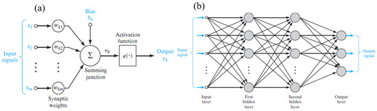
Figure 1.
(a) Perceptron model, labelled k [35], and (b) two hidden-layer MLPANN [37].
: the sum of the weighted inputs;
: the output of the kth perceptron;
: the jth synaptic weight sent to the kth preceding neuron;
: the jth input from the preceding neuron;
: the bias of the kth neuron which is a constant;
: the activation function.
Despite the simplicity of the mathematical model of the perceptron, which is the primitive model of the artificial neuron, it can efficiently model highly nonlinear engineering problems. This satisfaction comes from the principle of “Divide and Conquer”. This principle deals with a complex problem by dividing it into several minor problems and attacks each problem separately. By adopting this strategy, combining simple processing units in a network can definitely deal with highly complicated problems efficiently. In particular, a multi-layer perceptron artificial neural network (MLPANN), known in the AI field as the ANN, is an example of this strategy. In an MLPANN, every layer is composed of many single units, and the outputs of every layer are transmitted to the next layer and so on until the final output is calculated at the last layer. The first and last layers are assigned to the inputs and outputs, respectively, while the in-between layers are hidden. It is worth mentioning that the number of hidden layers and the number of their units are problem-specific, and they can be determined by a trial-and-error technique to identify the optimal numbers. The feed-forward neural network (FFNN) is one of the ANN architectures, and it is considered in this study. The FFNN layout is shown in Figure 1b [37]. Generally speaking, the most important issue in dealing with the ANN is the determination of the best set of synaptic weights. Usually, this issue is considered an optimization problem. Therefore, the network is trained using a set of input–output experimental data to obtain the required weights’ vector that satisfies the minimum mean squared errors (MSE) between the experimental output and the network’s output. This learning procedure is called a supervised-learning technique. The most common analytical algorithm that is used to train the FFNN is back-propagation (BP). However, the ANN can also be trained by integrating other recent and modern optimization algorithms, such as GA, PSO, ACO, etc.
2.2. ANFIS Model
The concept of fuzzy sets first appeared in the mid-sixties of the last century by Lotfi Zadeh [38]. He extended and generalized the classical binary set that is composed of only two values {0, 1} to accept elements with multi-degree memberships in the range [0 1]. This new concept needed new types of logic and algebra similar to Boolean logic and Boolean algebra. Therefore, fuzzy logic (FL) and fuzzy mathematics emerged. Nevertheless, this concept is extended to fuzzy numbers, fuzzy inference, fuzzy rules, etc. The work with the fuzzy set is analogical to the real-life way of thinking. In a binary set, the sharp threshold is applied to the membership degree of its instances. With this threshold, any element either belongs (takes a value of 1) or does not belong (takes a value of 0) to the set. However, in fuzzy sets, partial membership is possible. This partial degree of membership is very natural to match our real-life style. In this regard, the representation of an event might take a value of 0.3 or 0.8 depending on its degree of belonging to such a set through predefined membership functions (MFs). Therefore, partial belonging to multiple sets at the same time is valid in the concept of fuzzy sets.
The development of fuzzy systems first emerged by applying fuzzy logic in engineering applications in the mid-seventies of the last century by Ebrahim Mamdani. Professor Mamdani proposed the Mamdani-type fuzzy rule that takes the form as shown in Equation (3) [39]:
where a and b are the input variables; c is the output variable and A, B and C are the MFs of a, b and c, respectively.
IF a is A and b is B THEN c is C
The second keystone in the development of fuzzy systems is the Sugeno-type fuzzy rule which was proposed by Takagi, Sugeno and Kang (TSK) and takes the form as in Equation (4) [39]:
where a and b are the input variables; c is the output variable; A and B are the MFs of inputs a and b, respectively, and f(a, b) is a mathematical function of the inputs.
IF a is A and b is B THEN c = f(a, b)
In 1993, Kang proposed the adaptive network-based fuzzy inference system, ANFIS [40]. The ANFIS is a product of the collaboration between the FL and the ANN to mimic the fuzzification, inference engine and defuzzification processes. Consequently, the ANFIS is emulated in a networked structure as the same as the ANN, as shown in Figure 2. The fuzzification and the defuzzification processes are responsible for converting the crisp values of the variables to fuzzy values and vice versa, respectively. The inference engine is responsible for producing the final output by inferring the output of each individual rule through a Min operator and then aggregating these outputs to deliver the final single output through a Max operator. This inference technique is called the Min–Max procedure. The optimal parameters of the MFs and the weights of the connected network are determined through a training algorithm. The ANFIS is usually trained through a supervised learning procedure that uses a hybrid algorithm including the gradient descent (GD) and the least squares estimate (LSE). However, other modern optimization techniques can also be applied to ANFIS training.
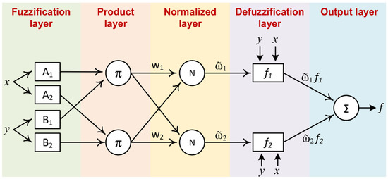
Figure 2.
The networked structure of the ANFIS.
2.3. LSTM Model
Long short-term memory (LSTM) is one of the artificial intelligence and deep learning tools that proved its efficiency in prediction models. It was first proposed by Hochreiter and Schmidhuber in 1997 [41]. It can be considered a higher version of the classical recurrent neural network (RNN). However, LSTM overcomes one of the main drawbacks of using the RNN, which is known as the vanishing gradient problem [42]. The RNN is a variant of neural networks that takes the past value of the output to be truncated with the present inputs vector to produce the future value of the output. It suffers from the premature convergence problem when the optimizer gets stuck in the local optima during the training process. This occurs when the gradient is getting smaller and smaller and hence produces an unchanged weight vector. LSTM sorted out this problem by taking into consideration the significant data samples even if it has been seen for a long time. Therefore, the working mechanism of the LSTM network is composed of three gates: the forget gate, the input gate and the output gate. Despite the first gate being called the forget gate, it is actually responsible for memorising significant data from the past. The structure of the LSTM network (cell) with its operational gates is shown in Figure 3.
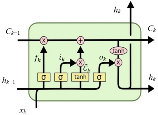
Figure 3.
Structure of the LSTM network with its operational gates.
Equations (5)–(10) describe the working operations of the LSTM cell as follows [43]:
where and are the responses of the forget, input and output gates, respectively; k is a time index; and are the network’s input and output vectors, respectively; and are the weight vectors associated with the input and output vectors of the gate n, respectively; denotes the network’s state; is the sigma function that maps its inputs to the range [0 1], as in Equation (11) and is the hyperbolic tangent function that maps its inputs to the range [−1 1], as in Equation (12).
3. Data Preparation
In this study, the data were downloaded from the “Our World in Data” website [34]. This data repository recorded many data with different categories for every country in the world. However, this study is only interested in the data for the CO2 emissions in Saudi Arabia. The available data are in the range from 1936 to 2020, but the two years 1951 and 1952 are missing. Therefore, this study considered only the data in the range from 1953 to 2020, which ends up with 67 data samples. Figure 4 shows the plot of the collected CO2 emissions in Saudi Arabia within the considered yearly range. However, without effective monitoring and controlling of the tremendous increase, it will negatively contribute to the global warming problem not only in the Middle East region but also all over the world. It is clear from the figure that since 1966, the CO2 emissions in Saudi Arabia were increasing rapidly, and this matches with the third industrial revolution which started in 1950 by emerging the digital world, internet, computer programming and computer networks, etc.
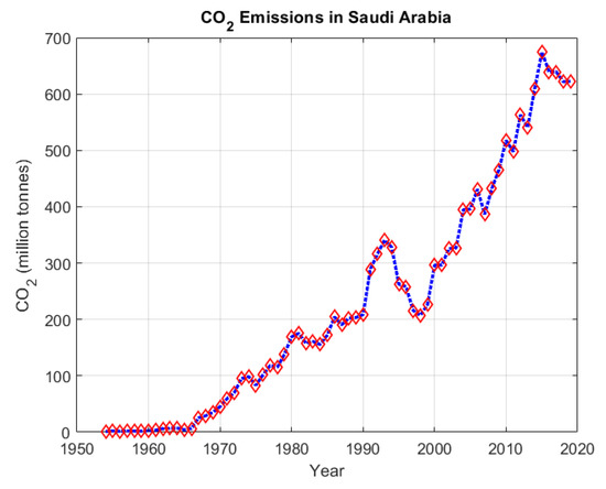
Figure 4.
The plot of yearly CO2 emissions in Saudi Arabia through 1953–2020.
This study addressed the selection of the data samples randomly for training and testing. In other words, to select random samples from the entire range for the training phase, the remaining samples were reserved for the testing phase. The ratio between the training and testing samples was set to 70:30 for all models. On the other hand, this study investigated the best input combination that produced the best performance. Table 2 illustrates the six groups of the input combination that have been examined in this study to predict the next value of the CO2 emission (CO2(t + 1)) in Saudi Arabia, where t is an index to the year.
Table 2.
The description of input combinations examined in this study.
The data are now ready for the modelling procedure. Therefore, in the following section, the methodologies of building the considered FFNN, ANFIS and LSTM models to forecast CO2 emissions in Saudi Arabia are described.
4. Results and Discussion
The available 67 data points were reformulated to be in an input–output data matrix form. For predicting the next sample from the present sample, the data matrix was prepared to have 66 data records. These records were divided into 46 samples for training, and the remaining 20 samples were held for testing with the optimal ratio of 70:30, respectively. The code was built using MATLAB R2022 in an intel CORE i7, 8 MB RAM computer, and the findings of the current work are presented in the following subsections. The obtained results from the addressed AI models will be presented in the following subsections.
4.1. FFNN
The study of predicting CO2 in Saudi Arabia included the feed-forward neural network (FFNN) as one of the artificial intelligence tools that proved its efficiency in many engineering applications [44]. Despite the FFNN’s success in pattern recognition applications in the field of data classification, it also produces a completive result in case of data regression problems. Therefore, the FFNN was nominated in this study as the first AI tool. Before starting the modelling phase, the input–output data were normalized to be in the range [0 1] by dividing the whole data set by the maximum value of the input and output vectors. This normalization procedure is beneficial for the learning phase because it unifies the inputs’ ranges to the learning algorithm while looking for the optimal weights’ vector. For a fair comparison, the FFNN model was trained with the same optimal training-to-testing ratio of 70:30. The structure of the network included n-input and single output architecture with one hidden layer that contained ten perceptrons (units). The number of inputs, n, was dependent on the input combination (number of inputs in the group) to be studied. The network was trained with the backpropagation (BP) algorithm for 10 epochs until the lowest RMSE value for the testing data was reached. Table 3 presents the resulting RMSE and R2 as comparison statistical measures for the training and testing phases.
Table 3.
The RMSE and the coefficient of determination for the training and testing data of the FFNN model.
The table illustrates that the input combinations in groups (Gr. #1, Gr. #4 and Gr. #6) are the best three groups that produced the minimum average RMSE and the maximum R2 values. Figure 5 presents the plots of the resulting outputs of the FFNN.
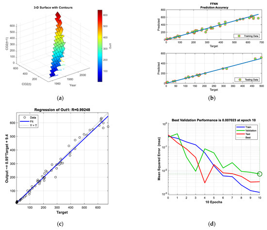
Figure 5.
The modelling results of the FFNN: (a) 3D surface, (b) training and testing prediction accuracies, (c) regression curve and (d) MSE of performance curves.
The prediction accuracy plot shown in Figure 5b demonstrates the good modelling phase where the model’s outputs are very close to the measured data samples for both training and testing subsets. These prediction accuracies are reinforced by the regression curve shown in Figure 5c, which shows that the FFNN has been trained correctly, and its output has more than a 99% correlation value with the measurements. Figure 5d illustrates also the convergence curves during the training phase, and it shows that the network is well-trained after 10 epochs. To show the entire performance of the FFNN model, the model predictions of the whole data set were plotted versus the experimental data points, as shown in Figure 6. The curves in Figure 6 show that the predicted output of the FFNN is very close to the measured data and tracks it well, which indicates the success of the training phase.
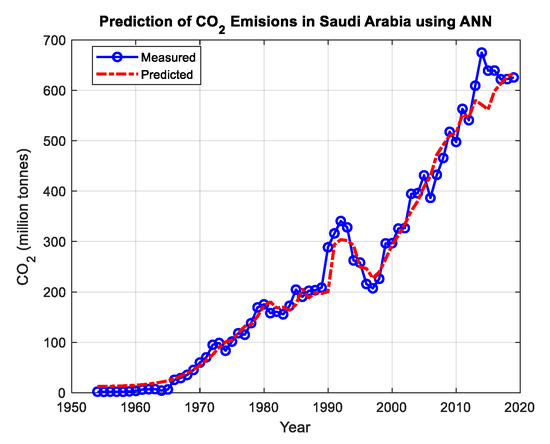
Figure 6.
The predictions of CO2 emissions in Saudi Arabia using the FFNN model from 1954–2020.
4.2. ANFIS
The ANFIS model parameters were assigned as the Gaussian-shape, the subtractive clustering (SC) and the weighted average (Wavg) for the fuzzification, rules generation and defuzzification processes, respectively. For obtaining a smoother prediction curve, the Gaussian-shape is a very suitable MF, as it gives a fine transition from one predicted point to the next. On the contrary, the other triangular or trapezoidal shapes produce jumps in the predictions. On the other hand, the SC technique produced the optimal as well as the smallest number of rules that can effectively handle the trend of the dataset. The ANFIS structure used in this work is the Sugeno-type fuzzy model. In this type, each rule considers the consequence (output) as a linear function of the antecedent (inputs). Accordingly, the defuzzification method aggregates the outputs by obtaining the weighted average of each rule to end up with a final single-valued output. To build a robust model, the process of continuous training was conducted for the ANFIS model until a stopping criterion was met. In this study, the training process stopped when the testing data’s root mean squared error (RMSE) reached the minimum value. The statistical markers were calculated in both phases to assess the performance of the resulting model in each phase. Table 4 illustrates the values of the root mean squared error (RMSE), coefficient of determination (R2) and number of generated fuzzy rules (#Rules). The first metric (RMSE) measures the accuracy of the model’s predictions, while the latter (R2) measures the tracking capability. The model is said to be better when its predictions give the lowest RMSE and the biggest R2 values for both groups of datasets (training and testing). R2 is defined as the squared of the correlation coefficient, which implies that its value is in the range [0 1] where 0 and 1 indicate no correlation and full correlation between the predicted and actual signals, respectively. By referring to Table 4 and according to the list of the lowest three average values and the list of the highest three coefficients of determination, it can be noticed that there are three input combinations shared between the two lists. The first combination is the year and the present value (Gr. #4), the second combination is the year and present value and its rate of change (Gr. #5), while the third combination is the year with the present value and the two past values (Gr. #6).
Table 4.
The RMSE and the coefficient of determination for the training and testing data of the fuzzy model.
In the randomly selected sets of training and testing samples, the fuzzy modelling succeeded in obtaining the better model. This is because the subtractive clustering algorithm used the entire range of the input samples. On the contrary, when using sequential data sets for training and testing, the fuzzy model builds its rules based on a part of the entire range, and hence, it is difficult for it to predict data far from this trained range. It can be noticed from Table 4 that in fuzzy modelling, adding the time index to a group of inputs keeps the temporal feature to the data and hence enhances the values of average prediction and the R2. This is clear when comparing the average and R2 values obtained from (Gr. #1, Gr. #4) and (Gr. #2, Gr. #5) with those obtained from (Gr. #3, Gr. #6). The fuzzy model structure and the membership functions of the input combination Gr. #4 are shown in Figure 7a,b, respectively. The training and testing predictions of the ANFIS model are plotted against the first and second inputs and are shown in Figure 8a,b, respectively. However, the training and testing prediction errors plotted against the first and second inputs are shown in Figure 8c,d, respectively. The model predictions are noticed to be well-matched with the measured samples for both training and testing subsets. This is supported by the prediction accuracy curve plotted in Figure 9a. The 3D surface shown in Figure 9b is also generated to illustrate the dependency and behaviour of the output on the variation of the inputs. For more inspection of the ANFIS model predictions, the predictions in both training and testing subsets were plotted in 3D view, as shown in Figure 10a,b, respectively.
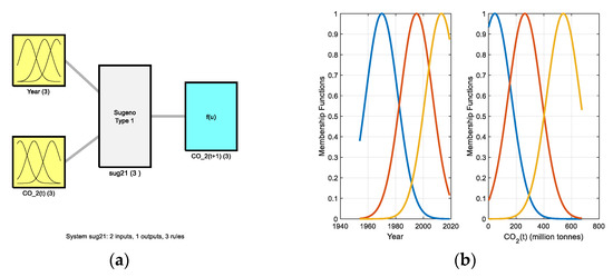
Figure 7.
(a) The structure of the fuzzy model and (b) the membership functions of the input combination in the case of Gr. #4.
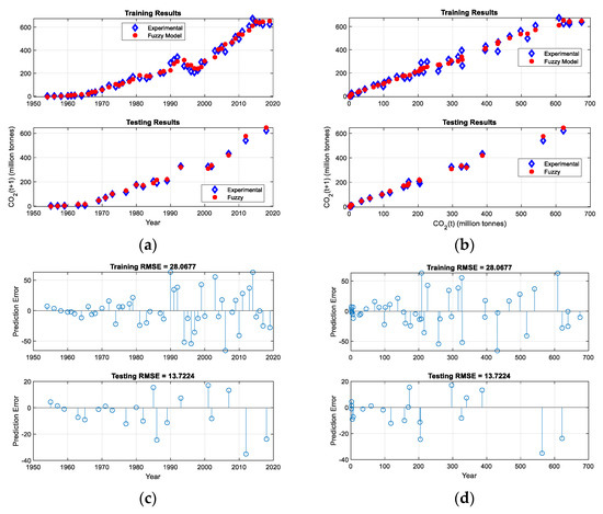
Figure 8.
The plots of the fuzzy model performance vs. the experimental data in case of Gr. #4 (a) training and testing performances against the first input, (b) training and testing performances against the second input, (c) training and testing prediction errors against the first input, (d) training and testing prediction errors against the second input.
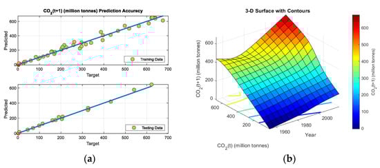
Figure 9.
(a) The fuzzy model’s prediction accuracy of training and testing data. (b) The fuzzy model 3D surface.
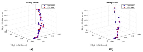
Figure 10.
The fuzzy model’s predictions vs. experimental measurements in 3D view: (a) training and (b) testing.
To show the entire performance of the ANFIS model, the model predictions of the whole data set were plotted versus the experimental data points, as shown in Figure 11.

Figure 11.
The predictions of CO2 emissions in Saudi Arabia using the ANFIS model from 1954–2020.
The curves in Figure 11 show that the predicted output of the ANFIS is very close to the measured data and tracks it efficiently, which indicates a successful training phase.
4.3. LSTM
Before the training procedure starts, the data is standardised with its mean and standard deviation as follows:
where and are the data sample and its standardized value at time t, respectively. and are the mean and standard deviation values of the training dataset.
Table 5 introduces the resulting RMSE and the R2 values obtained through the training and testing phases for the LSTM model. By referring to Table 5 and according to the list of the lowest three average values and the list of the highest three coefficients of determination, the three best groups are Gr. #2, Gr. #4 and Gr. #6.
Table 5.
The RMSE and the coefficient of determination for the training and testing data of the LSTM model.
Figure 12 illustrates the plots of the predicted samples using LSTM against the observed (real) data for both training and testing samples of Gr. #4. Figure 13 presents the errors between the LSTM predictions and the real data of the randomly selected subsets for the same input group. The lowest training and testing RMSE values resulting from the modelling phase were found to be 17.2924 and 13.5535, respectively, which occurred at Gr. #4.
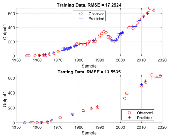
Figure 12.
The plots of the LSTM predictions against the real data for training and testing samples when the inputs are the year and the present value.
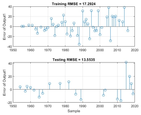
Figure 13.
The errors between the LSTM predictions and the real data in the case of random selection strategy when the inputs are the year and the present value.
To show the entire performance of the LSTM model, the model predictions of the whole data set were plotted versus the experimental data points, as shown in Figure 14. The curves in Figure 14 show that the predicted output of the LSTM model is very close to the measured data and tracks it well, which implies that the training phase was successful.
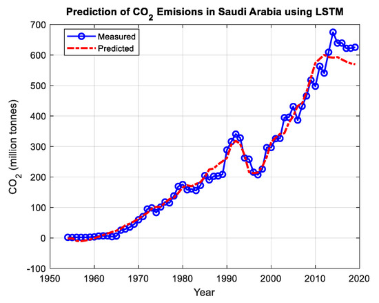
Figure 14.
The predictions of CO2 emissions in Saudi Arabia using the LSTM model from 1954–2020.
Referring to Table 3, Table 4 and Table 5, it can be concluded that input combination #4 is common in the best results list for the three LSTM, ANFIS and FFNN models. Therefore, the investigation study will be focused only on Gr. #4. Figure 15 shows the predictions of every individual model of the three considered AI models and their forecasting curves until the year 2030. Based on the FFNN forecasting curve, the CO2 emissions will remain constant with a slight change for the next ten years. However, the ANFIS forecasting model predicts that the emissions will increase for the next ten years but at a smaller rate than in the previous period. On the other hand, the LSTM expects that the curve will decrease for a while and then start to increase again.
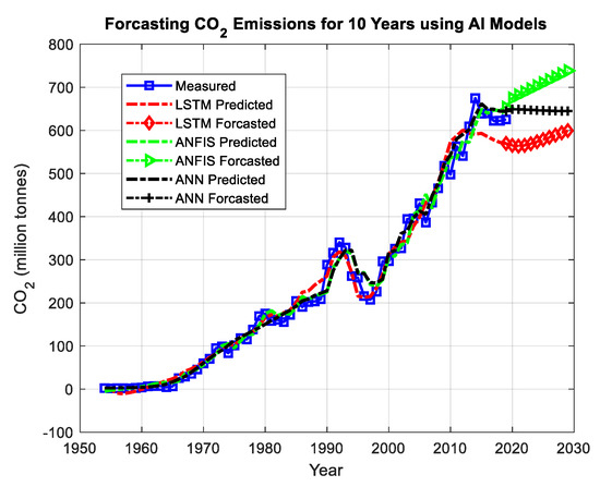
Figure 15.
The forecasting curves of CO2 emissions in Saudi Arabia using FFNN, ANFIS and LSTM.
For Gr. #4, the percentage of the mean absolute error (MAPE) to the average of the testing data for the FFNN, ANFIS and LSTM models were calculated, and their values were found to be 2.939%, 2.82% and 10.6881%, respectively.
5. Ensembled Model
Based on the “no free lunch” principle, a single model cannot have the power of two united models. In this study, the overall decision was considered with the ensemble of the three AI models’ responses to benefit from the collaboration of these models. This ensemble is represented by the average value of their outputs to end up with the final single decision, as shown in Figure 16. For the entire data set, the RMSE and the R2 values were calculated for each individual model as well as their averages. Table 6 presents the statistical markers of the RMSE and the R2 for the three considered AI models and their average values. It can be noticed that the RMSE of the ensemble model is the lowest among any individual model. Furthermore, the resulting output of the ensembled model is more correlated with the measured data than the output of any individual model based on the highest R2 value. The experimental data and the prediction values of the three models and their ensemble from 1954–2030 are tabulated in Table A1 in Appendix A.
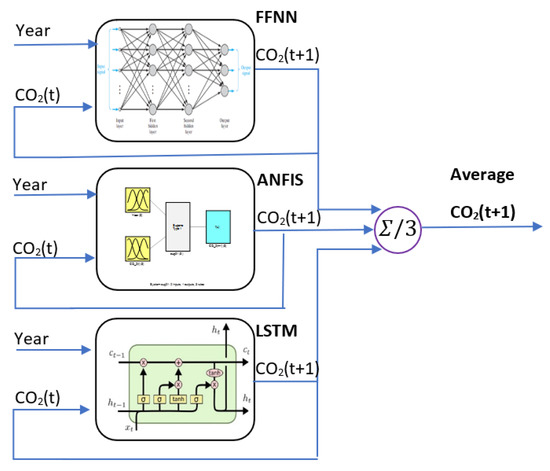
Figure 16.
The diagram of the forecasting ensemble of the three AI models.
Table 6.
The RMSE and R2 of the considered models’ responses and their average.
Figure 17 shows the predictions of the three AI models and their forecasting curves until the year 2030. The figure shows the average value of the ensembled model. From the average value curve, it can be noticed that with the current strategy, the CO2 emissions are expected to be increased but at a slight rate. From the available measurements, the increment in CO2 emissions was 9.4976 million tonnes/year in the period from 1953 to 2020. However, according to results from the AI models, it is expected that the increment will be only 6.1707 million tonnes/year in the period from 2020 to 2030. This implies that the increment rate decreases by 35.03%. This supports the strategy that the Saudi Arabian authorities adopted in order to decrease CO2 emissions to reach net zero by 2060. Eventually, the findings of this study and the predictions of the artificial intelligence models suggest that keeping the rate decrement within 35% every 10 years would help in reaching net zero by 2060 or before.
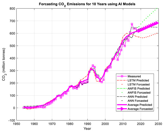
Figure 17.
Predictions of the AI models and their forecasting responses up to the year 2030.
To obtain a robust model, the possibility of the occurrence of overfitting has to be avoided. Thus, two strategies have been adopted in our research. The first one is to use an appropriate ratio between the training and testing samples to perform the training phase properly. In system modelling and machine learning fields, the ratio of 80:20 is commonly used [45]. In this regard, Joseph proposed a criterion for calculating the optimal training/testing splitting ratio, Rs, based on the number of parameters, n. Accordingly, this ratio is calculated as shown in Equation (14) [33]:
Therefore, by following this criterion and with the number of input parameters , the optimal training/testing ratio should be 70/30, which was adopted in our study. The second strategy is to assess the model predictions during the testing phase via the values of the statistical markers of RMSE and R2. Small and big RMSE and R2 values, respectively, indicate a successful training phase. Subsequently, the obtained model is reliable and can produce trustable predictions.
The models’ predictions have been validated with an unseen record of CO2 emissions in Saudi Arabia. This measurement has recently been added to the database repository to express emissions in the year 2021, which has a value of 672.38 tonnes. The measured, predicted and average values of this validation record when applying the FFNN, ANFIS and LSTM models are illustrated in Table 7. Moreover, the prediction error percentages obtained by these models, including their ensemble, are introduced in Table 8. From Table 8, it can be noticed that the ANFIS model produced the best prediction accuracy with the lowest error value of 0.3704%. On the other hand, the LSTM model had the highest prediction error value that reached 15.9288%. However, the FFNN presented a moderate error value of 638.4638%. Consequently, the percentage error value of the model’s ensemble was only 6.8675%, which implies that a forecasting accuracy of 93.1325% has been gained. These obtained high-accuracy predictions proved the reliability of the adopted forecasting strategy of using artificial intelligence tools as a forecasting ensemble. By comparing our findings with the other previous works, it is noticed that the results obtained by our suggested ensemble are better than those obtained by a recent study of forecasting CO2 emissions in the USA. This study produced a forecasting accuracy and prediction error of 92.42% and 7.58%, respectively [25]. However, our proposed methodology produced accuracy and error values of 93.1325% and 6.8675%, respectively. Furthermore, our results are compared with the one obtained in [14]. The LSTM model in [14] produced prediction RMSE and R2 values of 60.635 and 0.990, respectively, while our LSTM model delivers values of 15.42295 and 0.9945, respectively. This indicates that our suggested strategy is outstanding and promising. Usually, a forecasting model is classified according to its resulting percentage error as inaccurate, reasonable, good or highly accurate when the percentage error is greater than 50%, 20–50%, 10–20% and less than 10%, respectively [46]. Therefore, the proposed FFNN and ANFIS can be classified as highly accurate models, while the LSTM model can be considered good. In addition, as our proposed ensemble produced a validating error of 6.8675%, it can certainly be classified as a highly accurate forecasting model.
Table 7.
The measured, predicted and average values of the validating data obtained by the considered AI models.
Table 8.
The prediction errors of the validation record obtained by the considered AI models.
In conclusion, the main contribution of this work can be summarized in the following points, which makes it novel:
- An ensemble of three AI models, namely, FFNN, ANFIS and LSTM, has been built to forecast CO2 emissions in Saudi Arabia during the period from 2020 to 2030.
- The optimal train/test ratio of 70:30 was used throughout the training phase [33].
- The ensemble produced a forecasting error percentage of 6.8675% for the validating sample.
- The forecasting models are classified as highly accurate based on the formula in [46].
6. Conclusions
Tracking carbon dioxide (CO2) emissions obtained major interest all over the world in order to effectively monitor global warming. Therefore, this work presents a study of using artificial intelligence (AI) tools to forecast CO2 emissions in Saudi Arabia, the biggest fossil fuels exporter in the world, through the period from the year 2020 to 2030. Three powerful AI prediction models have been applied in this study. These models include the feed-forward neural network (FFNN), the adaptive network-based fuzzy inference system (ANFIS) and long short-term memory (LSTM). The annual measurements of CO2 emissions cover the period from 1936 to 2020 but with some missing values. The dataset was filtered to cover only the period from 1954 to 2020. For all models, the available records were divided randomly with the optimal ratio of 70:30 into two groups for training and testing, respectively. Every model was trained until the lowest root mean squared error (RMSE) of the testing data was obtained. The study also investigated the best input combination that produces the best performance. The predicting models’ performances have been assessed based on the smallest RMSE and the biggest coefficient of determination (R2) values. The group containing the past value and the temporal annual index year was found to be the best combination. The FFNN, ANFIS and LSTM produced average RMSEs of 19.78, 20.89505 and 15.42295, respectively, while the averages of R2 were found to be 0.990985, 0.98875 and 0.9945, respectively. The final predicted output was considered as the ensembled (average) value of the outputs resulting from the three AI models. The ensemble was validated with a new measurement of the year 2021, and the calculated percentage error was found to be 6.8675% with an accuracy of 93.1325%, which implies that the model is highly accurate. According to the ensemble forecasting values, the rate of CO2 emissions is expected to decrease in Saudi Arabia from 9.4976 million tonnes per year in the period 1954:2020 to 6.1707 million tonnes per year in the period 2020–2030. This implies that the increment rate will decrease by 35.03%. Accordingly, this result will definitely encourage and help policymakers to take the right action not only for the near future but also for the far future. The findings of this study suggest that keeping the decrement rate within 35% every 10 years will help in reaching net zero CO2 emissions in Saudi Arabia by 2060 or even before. In future work, another different ML tool, such as a regression support vector machine (RSVM), can be studied and included in the ensemble to increase the entire model’s prediction accuracy. Furthermore, the model’s predictability can be enhanced by restraining these models with any new annual measurements that might be added to the database.
Author Contributions
Conceptualization, A.M.N. and H.R.; methodology, A.M.N. and H.R.; software, A.M.N. and H.R.; validation, A.M.N., A.G.O., H.R. and M.A.A.; formal analysis, A.M.N., A.G.O., H.R. and M.A.A.; investigation, A.M.N., A.G.O., H.R. and M.A.A.; resources, A.M.N.; data curation, A.M.N. and H.R.; writing—original draft preparation, A.M.N., A.G.O., H.R. and M.A.A.; writing—review and editing, A.M.N., A.G.O., H.R. and M.A.A.; visualization, A.M.N., A.G.O., H.R. and M.A.A.; supervision, A.M.N.; project administration, A.M.N.; funding acquisition, A.M.N. All authors have read and agreed to the published version of the manuscript.
Funding
The authors extend their appreciation to the Deputyship for Research and Innovation, Ministry of Education in Saudi Arabia for funding this research work through the project number (IF2/PSAU/2022/01/22030).
Conflicts of Interest
The authors declare no conflict of interest.
Nomenclature
| Abbreviation | Description |
| ACO | Ant colony optimization |
| AI | Artificial intelligent |
| ANFIS | Adaptive neuro-fuzzy inference system |
| ANN | Artificial neural networks |
| ANOVA | Analysis of variance |
| ARIMA | Autoregressive integrated moving average |
| BP | Back-propagation |
| CNN | Convolution neural network |
| CO2 | Carbon dioxide |
| DL | Deep learning |
| FFNN | Feed-forward neural network |
| GA | Genetic algorithm |
| GDP | Gross domestic product |
| GPs | Gaussian processes |
| LMDI | Logarithmic mean division index |
| MAPE | Mean absolute percentage error |
| ML | Machine learning |
| MLPANN | Multi-layer perceptron artificial neural network |
| MSE | Mean squared errors |
| PSO | Particle swarm optimization |
| R2 | Coefficient of determination |
| RMSE | Root mean squared errors |
| RNN | Recurrent neural network |
| RSVM | Regression support vector machine |
| SARIMAX | Seasonal autoregressive integrated moving average with exogenous factors |
| STSM | Structural time-series model |
| UEDT | Underlying energy demand trend |
Appendix A
Table A1.
Original and AI models’ predictions data for the CO2 emissions in Saudi Arabia from 1954–2030.
Table A1.
Original and AI models’ predictions data for the CO2 emissions in Saudi Arabia from 1954–2030.
| Original Data | Predicted CO2(t + 1) | |||||
|---|---|---|---|---|---|---|
| Inputs | Output | AI Models’ Predictions | ||||
| t(Year) | CO2(t) | CO2(t + 1) | FFNN | ANFIS | LSTM | AVERAGE |
| 1954 | 1.238 | 2.114 | 12.50611 | −5.08987 | −2.01652 | 1.799911 |
| 1955 | 2.114 | 1.63 | 12.679 | −2.75545 | −1.02799 | 2.965184 |
| 1956 | 1.63 | 2.099 | 12.89792 | −1.4773 | −9.73667 | 0.561316 |
| 1957 | 2.099 | 1.997 | 13.2161 | 0.542316 | −10.5423 | 1.072047 |
| 1958 | 1.997 | 1.854 | 13.63345 | 2.119091 | −8.34127 | 2.470423 |
| 1959 | 1.854 | 2.674 | 14.19032 | 3.665127 | −5.0274 | 4.276015 |
| 1960 | 2.674 | 3.568 | 14.95435 | 5.961256 | −0.62737 | 6.762744 |
| 1961 | 3.568 | 6.25 | 15.96297 | 8.316796 | 4.074516 | 9.451427 |
| 1962 | 6.25 | 6.939 | 17.34324 | 12.06533 | 9.549446 | 12.986 |
| 1963 | 6.939 | 7.041 | 19.06351 | 14.2668 | 14.49436 | 15.94156 |
| 1964 | 7.041 | 4.216 | 21.25589 | 16.01483 | 19.63215 | 18.96763 |
| 1965 | 4.216 | 6.407 | 23.88634 | 15.48812 | 24.05496 | 21.14314 |
| 1966 | 6.407 | 25.485 | 27.48476 | 18.87039 | 30.33186 | 25.56233 |
| 1967 | 25.485 | 29.079 | 33.15059 | 35.42178 | 41.40516 | 36.65918 |
| 1968 | 29.079 | 35.271 | 38.87615 | 39.9241 | 46.89222 | 41.89749 |
| 1969 | 35.271 | 45.251 | 45.87024 | 46.47104 | 54.6504 | 48.99723 |
| 1970 | 45.251 | 59.757 | 54.38627 | 56.00684 | 63.27654 | 57.88989 |
| 1971 | 59.757 | 70.282 | 64.68987 | 69.13748 | 73.45562 | 69.09432 |
| 1972 | 70.282 | 95.054 | 75.49803 | 79.21233 | 82.22738 | 78.97924 |
| 1973 | 95.054 | 98.702 | 89.86426 | 100.6304 | 96.3252 | 95.60662 |
| 1974 | 98.702 | 83.261 | 100.8192 | 105.461 | 102.1858 | 102.822 |
| 1975 | 83.261 | 101.46 | 104.6741 | 95.16006 | 102.069 | 100.6344 |
| 1976 | 101.46 | 118.07 | 118.4744 | 111.7087 | 115.6099 | 115.2643 |
| 1977 | 118.07 | 115.025 | 131.8265 | 127.1765 | 127.5863 | 128.8631 |
| 1978 | 115.025 | 138.005 | 135.3067 | 126.9572 | 132.2368 | 131.5002 |
| 1979 | 138.005 | 169.24 | 151.2927 | 147.8069 | 147.6745 | 148.9247 |
| 1980 | 169.24 | 175.305 | 172.9232 | 175.0902 | 165.833 | 171.2822 |
| 1981 | 175.305 | 157.893 | 180.114 | 182.1811 | 172.8314 | 178.3755 |
| 1982 | 157.893 | 160.837 | 168.4436 | 170.9286 | 169.5612 | 169.6445 |
| 1983 | 160.837 | 155.512 | 169.7221 | 175.6413 | 177.098 | 174.1538 |
| 1984 | 155.512 | 172.421 | 163.3358 | 173.8981 | 183.0917 | 173.4419 |
| 1985 | 172.421 | 204.604 | 175.3805 | 189.1726 | 200.2302 | 188.2611 |
| 1986 | 204.604 | 190.447 | 206.4798 | 214.9121 | 224.8404 | 215.4108 |
| 1987 | 190.447 | 202.252 | 187.7666 | 206.7261 | 227.6711 | 207.3879 |
| 1988 | 202.252 | 203.424 | 198.4083 | 217.1242 | 241.2667 | 218.9331 |
| 1989 | 203.424 | 208.497 | 196.9009 | 219.8459 | 251.2149 | 222.6539 |
| 1990 | 208.497 | 288.546 | 200.3989 | 225.2428 | 262.3358 | 229.3259 |
| 1991 | 288.546 | 316.175 | 294.0228 | 281.6761 | 305.9605 | 293.8864 |
| 1992 | 316.175 | 340.642 | 303.7727 | 302.1944 | 318.6143 | 308.1938 |
| 1993 | 340.642 | 328.139 | 302.1878 | 320.8028 | 308.4464 | 310.479 |
| 1994 | 328.139 | 262.421 | 292.5973 | 314.3748 | 270.5121 | 292.4948 |
| 1995 | 262.421 | 258.275 | 249.5026 | 271.1697 | 215.8058 | 245.4927 |
| 1996 | 258.275 | 215.807 | 246.4183 | 270.1953 | 212.6085 | 243.074 |
| 1997 | 215.807 | 207.24 | 227.3038 | 242.8541 | 214.6285 | 228.2622 |
| 1998 | 207.24 | 225.986 | 239.6036 | 238.7858 | 234.3291 | 237.5728 |
| 1999 | 225.986 | 296.364 | 265.2283 | 253.5679 | 265.5935 | 261.4632 |
| 2000 | 296.364 | 296.588 | 293.3954 | 305.8328 | 313.5931 | 304.2738 |
| 2001 | 296.588 | 325.698 | 312.3551 | 308.6746 | 328.8756 | 316.6351 |
| 2002 | 325.698 | 326.517 | 334.3511 | 334.7226 | 341.3091 | 336.7943 |
| 2003 | 326.517 | 394.585 | 360.4692 | 339.2313 | 343.7582 | 347.8196 |
| 2004 | 394.585 | 395.855 | 379.8552 | 405.7337 | 377.9214 | 387.8368 |
| 2005 | 395.855 | 431.292 | 408.6755 | 413.6198 | 399.3748 | 407.2234 |
| 2006 | 431.292 | 386.507 | 429.8014 | 452.2525 | 432.9277 | 438.3272 |
| 2007 | 386.507 | 432.336 | 472.5769 | 419.0285 | 441.094 | 444.2331 |
| 2008 | 432.336 | 465.844 | 491.8752 | 468.4847 | 479.0602 | 479.8067 |
| 2009 | 465.844 | 517.716 | 510.1533 | 500.8319 | 526.1445 | 512.3766 |
| 2010 | 517.716 | 497.659 | 514.9955 | 538.7184 | 573.7942 | 542.5027 |
| 2011 | 497.659 | 563.18 | 551.6828 | 535.1195 | 587.5349 | 558.1124 |
| 2012 | 563.18 | 540.805 | 546.4432 | 575.9426 | 600.6204 | 574.3354 |
| 2013 | 540.805 | 609.206 | 580.0512 | 572.1777 | 593.1379 | 581.7889 |
| 2014 | 609.206 | 674.878 | 571.6647 | 611.921 | 591.4464 | 591.6774 |
| 2015 | 674.878 | 639.056 | 561.8672 | 649.3612 | 593.2609 | 601.4964 |
| 2016 | 639.056 | 639.378 | 598.6502 | 639.9262 | 585.4526 | 608.0096 |
| 2017 | 639.378 | 621.953 | 613.3382 | 647.1517 | 578.1209 | 612.8703 |
| 2018 | 621.953 | 622.413 | 627.1504 | 646.1793 | 572.3751 | 615.2349 |
| 2019 | 622.413 | 625.508 | 634.0576 | 653.4732 | 569.892 | 619.1409 |
| 2020 | 625.508 | 672.38 | 638.4638 | 674.8708 | 565.2777 | 626.204 |
| 2021 | - | - | 642.2474 | 691.7801 | 563.9153 | 632.6476 |
| 2022 | - | - | 645.0641 | 706.6142 | 566.0118 | 639.23 |
| 2023 | - | - | 647.1015 | 720.4899 | 569.6484 | 645.7466 |
| 2024 | - | - | 648.4952 | 733.9226 | 573.9244 | 652.1141 |
| 2025 | - | - | 649.3532 | 747.15 | 578.4414 | 658.3149 |
| 2026 | - | - | 649.7565 | 760.2819 | 583.0188 | 664.3524 |
| 2027 | - | - | 649.762 | 773.3691 | 587.5727 | 670.2346 |
| 2028 | - | - | 649.4067 | 786.4351 | 592.0653 | 675.9691 |
| 2029 | - | - | 648.712 | 799.491 | 596.4827 | 681.5619 |
| 2030 | - | - | 647.6882 | 812.542 | 600.8256 | 687.0186 |
References
- Tollefson, J. Carbon emissions hit new high: Warning from COP27. Nature 2022. [Google Scholar] [CrossRef] [PubMed]
- Naddaf, M. ‘Actions, not just words’: Egypt’s climate scientists share COP27 hopes. Nature 2022. [Google Scholar] [CrossRef] [PubMed]
- Yao, S.; Yang, L.; Shi, S.; Zhou, Y.; Long, M.; Zhang, W.; Cai, S.; Huang, C.; Liu, T.; Zou, B. A Two-in-One Annealing Enables Dopant Free Block Copolymer Based Organic Solar Cells with over 16% Efficiency. Chin. J. Chem. 2023, 41, 672–678. [Google Scholar] [CrossRef]
- Liu, T.; Zhou, K.; Ma, R.; Zhang, L.; Huang, C.; Luo, Z.; Zhu, H.; Yao, S.; Yang, C.; Zou, B.; et al. Multifunctional all-polymer photovoltaic blend with simultaneously improved efficiency (18.04%), stability and mechanical durability. Aggregate 2022, e308. [Google Scholar] [CrossRef]
- Manvitha, M.S.; Vani Pujitha, M.; Prasad, N.H.; Yashitha Anju, B. A Predictive Analysis on CO2 Emissions in Automobiles using Machine Learning Techniques. In Proceedings of the 2023 International Conference on Intelligent Data Communication Technologies and Internet of Things (IDCIoT), Bengaluru, India, 5–7 January 2023; pp. 394–401. [Google Scholar]
- Li, Y.; Huang, S.; Miao, L.; Wu, Z. Simulation analysis of carbon peak path in China from a multi-scenario perspective: Evidence from random forest and back propagation neural network models. Environ. Sci. Pollut. Res. Int. 2023, 30, 46711–46726. [Google Scholar] [CrossRef]
- Li, G.; Yang, Z.; Yang, H. A new hybrid short-term carbon emissions prediction model for aviation industry in China. Alex. Eng. J. 2023, 68, 93–110. [Google Scholar] [CrossRef]
- Khajavi, H.; Rastgoo, A. Predicting the carbon dioxide emission caused by road transport using a Random Forest (RF) model combined by Meta-Heuristic Algorithms. Sustain. Cities Soc. 2023, 93, 104503. [Google Scholar] [CrossRef]
- Ma, N.; Shum, W.Y.; Han, T.; Lai, F. Can Machine Learning be Applied to Carbon Emissions Analysis: An Application to the CO2 Emissions Analysis Using Gaussian Process Regression. Front. Energy Res. 2021, 9, 756311. [Google Scholar] [CrossRef]
- Rahman, S.M.A.; Nassef, A.M.; Al-Dhaifallah, M.; Abdelkareem, M.A.; Rezk, H. The Effect of a New Coating on the Drying Performance of Fruit and Vegetables Products: Experimental Investigation and Artificial Neural Network Modeling. Foods 2020, 9, 308. [Google Scholar] [CrossRef]
- Rezk, H.; Mohammed, R.H.; Rashad, E.; Nassef, A.M. ANFIS-based accurate modeling of silica gel adsorption cooling cycle. Sustain. Energy Technol. Assess. 2022, 50, 101793. [Google Scholar] [CrossRef]
- Deraz, A.A.; Badawy, O.; Elhosseini, M.A.; Mostafa, M.; Ali, H.A.; El-Desouky, A.I. Deep learning based on LSTM model for enhanced visual odometry navigation system. Ain Shams Eng. J. 2022, 102050. [Google Scholar] [CrossRef]
- Camastra, F.; Capone, V.; Ciaramella, A.; Riccio, A.; Staiano, A. Prediction of environmental missing data time series by Support Vector Machine Regression and Correlation Dimension estimation. Environ. Model. Softw. 2022, 150, 105343. [Google Scholar] [CrossRef]
- Kumari, S.; Singh, S.K. Machine learning-based time series models for effective CO2 emission prediction in India. Environ. Sci. Pollut. Res. 2022. [Google Scholar] [CrossRef]
- Vlachas, P.R.; Byeon, W.; Wan, Z.Y.; Sapsis, T.P.; Koumoutsakos, P. Data-driven forecasting of high-dimensional chaotic systems with long short-term memory networks. Proc. R. Soc. A Math. Phys. Eng. Sci. 2018, 474, 20170844. [Google Scholar] [CrossRef] [PubMed]
- Amarpuri, L.; Yadav, N.; Kumar, G.; Agrawal, S. Prediction of CO2 emissions using deep learning hybrid approach: A Case Study in Indian Context. In Proceedings of the 2019 Twelfth International Conference on Contemporary Computing (IC3), Noida, India, 8–10 August 2019; pp. 1–6. [Google Scholar]
- Meng, Y.; Noman, H. Predicting CO2 Emission Footprint Using AI through Machine Learning. Atmosphere 2022, 13, 1871. [Google Scholar] [CrossRef]
- Komeili Birjandi, A.; Fahim Alavi, M.; Salem, M.; Assad, M.E.H.; Prabaharan, N. Modeling carbon dioxide emission of countries in southeast of Asia by applying artificial neural network. Int. J. Low-Carbon Technol. 2022, 17, 321–326. [Google Scholar] [CrossRef]
- Qi, Y.; Peng, W.; Yan, R.; Rao, G.; Hassanien, A.E.I.B. Use of BP Neural Networks to Determine China’s Regional CO2 Emission Quota. Complexity 2021, 2021, 6659302. [Google Scholar] [CrossRef]
- Abdullah, A.M.; Usmani, R.S.A.; Pillai, T.R.; Marjani, M.; Hashem, I.A.T. An Optimized Artificial Neural Network Model using Genetic Algorithm for Prediction of Traffic Emission Concentrations. Int. J. Adv. Comput. Sci. Appl. 2021, 12, 794–803. [Google Scholar] [CrossRef]
- Cansiz, O.F.; Unsalan, K.; Unes, F. Prediction of CO2 emission in transportation sector by computational intelligence techniques. Int. J. Glob. Warm. 2022, 27, 271. [Google Scholar] [CrossRef]
- Khan, M.Z.; Khan, M.F. Application of ANFIS, ANN and fuzzy time series models to CO2 emission from the energy sector and global temperature increase. Int. J. Clim. Chang. Strateg. Manag. 2019, 11, 622–642. [Google Scholar] [CrossRef]
- Faruque, M.O.; Rabby, M.A.J.; Hossain, M.A.; Islam, M.R.; Rashid, M.M.U.; Muyeen, S.M. A comparative analysis to forecast carbon dioxide emissions. Energy Rep. 2022, 8, 8046–8060. [Google Scholar] [CrossRef]
- Zhang, X.; Zhang, W. A Hybrid Daily Carbon Emission Prediction Model Combining CEEMD, WD and LSTM. In Intelligent Computing Methodologies: 18th International Conference, ICIC 2022, Xi’an, China, 7–11 August 2022, Proceedings, Part III; Springer International Publishing: Cham, Switzerland, 2022; pp. 557–571. [Google Scholar]
- Mutascu, M. CO2 emissions in the USA: New insights based on ANN approach. Environ. Sci. Pollut. Res. Int. 2022, 29, 68332–68356. [Google Scholar] [CrossRef]
- Wang, C.; Li, M.; Yan, J. Forecasting carbon dioxide emissions: Application of a novel two-stage procedure based on machine learning models. J. Water Clim. Chang. 2023, 14, 477–493. [Google Scholar] [CrossRef]
- Hamieh, A.; Rowaihy, F.; Al-Juaied, M.; Abo-Khatwa, A.N.; Afifi, A.M.; Hoteit, H. Quantification and analysis of CO2 footprint from industrial facilities in Saudi Arabia. Energy Convers. Manag. X 2022, 16, 100299. [Google Scholar] [CrossRef]
- Alam, T.; AlArjani, A. A Comparative Study of CO2 Emission Forecasting in the Gulf Countries Using Autoregressive Integrated Moving Average, Artificial Neural Network, and Holt-Winters Exponential Smoothing Models. Adv. Meteorol. 2021, 2021, 8322590. [Google Scholar] [CrossRef]
- Alajmi, R.G. Carbon emissions and electricity generation modeling in Saudi Arabia. Environ. Sci. Pollut. Res. 2022, 29, 23169–23179. [Google Scholar] [CrossRef]
- Habadi, M.I.; Tsokos, C.P. Statistical Forecasting Models of Atmospheric Carbon Dioxide and Temperature in the Middle East. J. Geosci. Environ. Prot. 2017, 5, 11–21. [Google Scholar] [CrossRef]
- Althobaiti, Z.F.; Shabri, A. Prediction of CO2 emissions in Saudi Arabia using Nonlinear Grey Bernoulli Model NGBM (1,1) compared with GM (1,1) model. J. Phys. Conf. Ser. 2022, 2259, 012011. [Google Scholar] [CrossRef]
- Alkhathlan, K.; Javid, M. Carbon emissions and oil consumption in Saudi Arabia. Renew. Sustain. Energy Rev. 2015, 48, 105–111. [Google Scholar] [CrossRef]
- Joseph, V.R. Optimal ratio for data splitting. Stat. Anal. Data Min. ASA Data Sci. J. 2022, 15, 531–538. [Google Scholar] [CrossRef]
- Ritchie, H.; Roser, M.; Rosado, P. CO2 and Greenhouse Gas Emissions. Available online: https://ourworldindata.org/co2-and-other-greenhouse-gas-emissions (accessed on 24 December 2022).
- Herculano-Houzel, S. The human brain in numbers: A linearly scaled-up primate brain. Front. Hum. Neurosci. 2009, 3, 31. [Google Scholar] [CrossRef] [PubMed]
- Haykin, S.A. Neural Networks: A Comprehensive Foundation; Prentice Hall: Hoboken, NJ, USA, 2008. [Google Scholar]
- Haykin, S.S. Neural Networks and Learning Machines/Simon Haykin; Prentice Hall: New York, NY, USA, 2009. [Google Scholar]
- Zadeh, L.A. Fuzzy sets. Inf. Control 1965, 8, 338–353. [Google Scholar] [CrossRef]
- Nassef, A.M.; Rahman, S.M.A.; Rezk, H.; Said, Z. ANFIS-Based Modelling and Optimal Operating Parameter Determination to Enhance Cocoa Beans Drying-Rate. IEEE Access 2020, 8, 45964–45973. [Google Scholar] [CrossRef]
- Jang, J.S.R. ANFIS: Adaptive-network-based fuzzy inference system. IEEE Trans. Syst. Man Cybern. 1993, 23, 665–685. [Google Scholar] [CrossRef]
- Hochreiter, S.; Schmidhuber, J. Long short-term memory. Neural Comput. 1997, 9, 1735–1780. [Google Scholar] [CrossRef]
- Hochreiter, S. The Vanishing Gradient Problem during Learning Recurrent Neural Nets and Problem Solutions. Int. J. Uncertain. Fuzziness Knowl.-Based Syst. 1998, 6, 107–116. [Google Scholar] [CrossRef]
- Luo, J.; Zhang, Z.; Fu, Y.; Rao, F. Time series prediction of COVID-19 transmission in America using LSTM and XGBoost algorithms. Results Phys. 2021, 27, 104462. [Google Scholar] [CrossRef]
- Rahman, S.M.A.; Rezk, H.; Abdelkareem, M.A.; Hoque, M.E.; Mahbub, T.; Shah, S.K.; Nassef, A.M. Predicting Drying Performance of Osmotically Treated Heat Sensitive Products Using Artificial Intelligence. Comput. Mater. Contin. 2021, 67, 3143–3160. [Google Scholar] [CrossRef]
- Gholamy, A.; Kreinovich, V.; Kosheleva, O. Why 70/30 or 80/20 Relation between Training and Testing Sets: A Pedagogical Explanation; University of Texas: El Paso, TX, USA, 2018. [Google Scholar]
- Lewis, C.D. Industrial and Business Forecasting Methods: A Practical Guide to Exponential Smoothing and Curve Fitting/Colin D. Lewis; Butterworth Scientific: London, UK, 1982. [Google Scholar]


Disclaimer/Publisher’s Note: The statements, opinions and data contained in all publications are solely those of the individual author(s) and contributor(s) and not of MDPI and/or the editor(s). MDPI and/or the editor(s) disclaim responsibility for any injury to people or property resulting from any ideas, methods, instructions or products referred to in the content. |
© 2023 by the authors. Licensee MDPI, Basel, Switzerland. This article is an open access article distributed under the terms and conditions of the Creative Commons Attribution (CC BY) license (https://creativecommons.org/licenses/by/4.0/).