Abstract
Coseismic landslides pose a significant threat to the sustainability of both the natural environment and the socioeconomic fabric of society. This escalation in earthquake frequency has driven a growing interest in regional-scale assessment techniques for these landslides. The widely adopted infinite slope model, introduced by Newmark, is commonly utilized to assess coseismic landslide hazards. However, this conventional model falls short of capturing the influence of rock mass structure on slope stability. A novel methodology was previously introduced, considering the roughness of potential slide surfaces on the inner slope, offering a fresh perspective on coseismic landslide hazard mapping. In this paper, the proposed method is recalibrated using new datasets from the 2013 Lushan earthquake. The datasets encompass geological units, peak ground acceleration (PGA), and a high-resolution digital elevation model (DEM), rasterized at a grid spacing of 30 m. They are integrated within an infinite slope model, employing Newmark’s permanent deformation analysis. This integration enables the estimation of coseismic displacement in each grid area resulting from the 2013 Lushan earthquake. To validate the model, the simulated displacements are compared with the inventory of landslides triggered by the Lushan earthquake, allowing the derivation of a confidence level function that correlates predicted displacement with the spatial variation of coseismic landslides. Ultimately, a hazard map of coseismic landslides is generated based on the values of the certainty factor. The analysis of the area under the curve is utilized to illustrate the improved effectiveness of the proposed method. Comparative studies with the 2014 Ludian earthquake reveal that the coseismic landslides triggered by the 2013 Lushan earthquake predominantly manifest as shallow rock falls and slides. Brittle coseismic fractures are often associated with reverse seismogenic faults, while complaint coseismic fractures are more prevalent in strike–slip seismogenic faults. The mapping procedure stands as a valuable tool for predicting seismic hazard zones, providing essential insights for decision-making in infrastructure development and post-earthquake construction endeavors.
1. Introduction
Landslide disasters usually cause significant loss of life and property damage [1,2]. Earthquakes are one of the primary triggers for landslides [3]. In recent years, a rise in strong earthquakes globally has resulted in frequent coseismic landslide hazards, causing great damage in mountainous areas, and posing a serious threat to social sustainability. Consequently, the evaluation of regional coseismic landslide hazards holds paramount importance for pre-earthquake urban planning and post-earthquake reconstruction efforts.
Early attempts to evaluate the coseismic stability of slopes involved the application of the pseudo-static analysis method [4] and the finite-element modeling technique [5]. Accurately predicting slope displacement is important for evaluating seismic slope stability [6,7]. Newmark [8] introduced a straightforward and effective method, still widely used today, for estimating the coseismic permanent displacements of slopes. The models for estimating the coseismic permanent displacements of slopes can be grouped into four categories: rigid-block model, decoupled model, coupled model, and unified model. Newmark’s original methodology is generally referred to as rigid-block analysis [9]. To enhance the accuracy of estimating earthquake-induced permanent displacement, a decoupled analysis was developed by Makdisi and Seed [10]. The decoupled analysis accounts for the deformation of the sliding block during the sliding process. Bray and Rathje [11] introduced a streamlined seismic displacement method by utilizing a fully nonlinear decoupled one-dimensional dynamic analysis technique in conjunction with Newmark’s rigid-plastic sliding block analysis. Rathje and Bray [12,13] conducted a comparative analysis, contrasting outcomes obtained through rigid-block analysis with both linear and nonlinear coupled as well as decoupled analyses. In the coupled method, deformation and displacement are considered simultaneously, offering a more realistic portrayal of slope response under seismic forces. Bray and Travasarou [14] proposed a simplified approach to predict earthquake-induced permanent displacement based on a nonlinear fully coupled sliding block model, incorporating critical acceleration, dominant sliding block period, and seismic spectral acceleration. Considering the variety in the natural period of the sliding mass during the dynamic response of slopes, a unified simplified model was developed for predicting earthquake-induced sliding displacements of rigid and flexible landslide masses [15]. Recently, Zhang et al. [16,17] introduced a novel model for evaluating seismic slope stability, considering the influence of velocity pulse seismic motion on permanent slope displacement, thereby presenting an advanced framework for assessing seismic slope stability under the specific influence of near-fault pulses.
Jibson et al. [18,19] elucidated the computational process of the Newmark method for the regional hazard mapping of coseismic landslides. This pioneering work significantly advanced the utilization and refinement of the Newmark method within the realm of regional coseismic landslide susceptibility analysis. Subsequently, numerous scholars have adopted and applied the Newmark method in their assessments of regional coseismic landslide susceptibility. Yuan et al. [20] applied the fundamental approach delineated by Jibson [18,19] to calculate the Newmark displacement of slopes using strong ground-motion recordings from the 2013 Lushan earthquake. Various empirical equations with updated fitting coefficients have been formulated for a comparative analysis of Newmark displacement estimation. Ma and Xu [21] introduced an approach that integrates logistic regression and support vector machine models with critical acceleration for the hazard assessment of landslides triggered by the 2013 Lushan earthquake. This method proves to be more effective in coseismic landslide hazard assessment compared to the simplified Newmark model. Jin et al. [22] modified the Newmark model by incorporating attenuation coefficients to the effective internal friction angle and the effective cohesion of geologic units. The coseismic landslide hazard zoning, derived from the modified Newmark model, exhibited a good correlation with the actual distribution of landslides triggered by the 2013 Lushan earthquake. In the context of the 2013 Lushan earthquake, Ma [23] demonstrated that the Newmark method’s rapid assessment, even without coseismic landslide data, adequately fulfills the spatial prediction requirements for coseismic landslides during the emergency response phase of disaster reduction.
Valley incisions frequently lead to the formation of shallow unloading joints parallel to the surface in natural slopes [24,25]. Research indicates that during strong earthquakes, rock slopes exhibit collapsing and sliding failures along these shallow unloading joints, with approximately 90% of coseismic landslides being shallow falls and slides [26,27,28,29]. Unstable rock blocks are frequently fragmented and mobilized along these joints [30]. However, prior studies have not sufficiently considered the shear strength of these rock joints when evaluating coseismic landslides. In addressing this gap, Zang et al. [31] incorporated the Barton model [32] into the Newmark method to enhance the estimation of slopes’ dynamic stability. The method was initially employed and calibrated to assess the hazards associated with coseismic landslides, utilizing data from the 2014 Ludian earthquake in Yunnan Province, southwestern China. The area under the curve analysis revealed that the reliability of the proposed method surpasses that of the conventional Newmark approach. The seismogenic fault associated with the 2014 Ludian earthquake is identified as the Baogunao–Xiaohe fault, characterized by left-lateral strike–slip movement [33]. Field investigations into coseismic landslides have brought to light significant disparities in the spatial distribution patterns between reverse-type and strike–slip-type seismogenic faults [29,34]. The failure modes of slopes exhibit variation in regions affected by different types of seismogenic faults, as do the corresponding calculation parameters. A limitation of the initial calibration lies in its exclusive reliance on coseismic landslides triggered by a strike–slip fault. To address this constraint, our study rigorously reevaluates the initial methodology and enhances its precision through recalibration. This is achieved by incorporating the coseismic landslide dataset from the 2013 Lushan earthquake, identified as a blind reverse-fault event [35]. Following calibration, the methodology becomes applicable for mapping the spatial distribution of coseismic landslides under various seismogenic fault conditions.
This paper provides a concise overview of the features and spatial distribution of landslides triggered by the 2013 Lushan earthquake within the study area, outlines the methodology employed to assess the stability of coseismic slopes, details the procedure for mapping coseismic landslide hazards, and concludes with a discussion of the coseismic hazard assessment results. The paper further compares these findings with those from our prior studies. Finally, it explores the limitations of the method and outlines potential avenues for future research.
2. Study Area
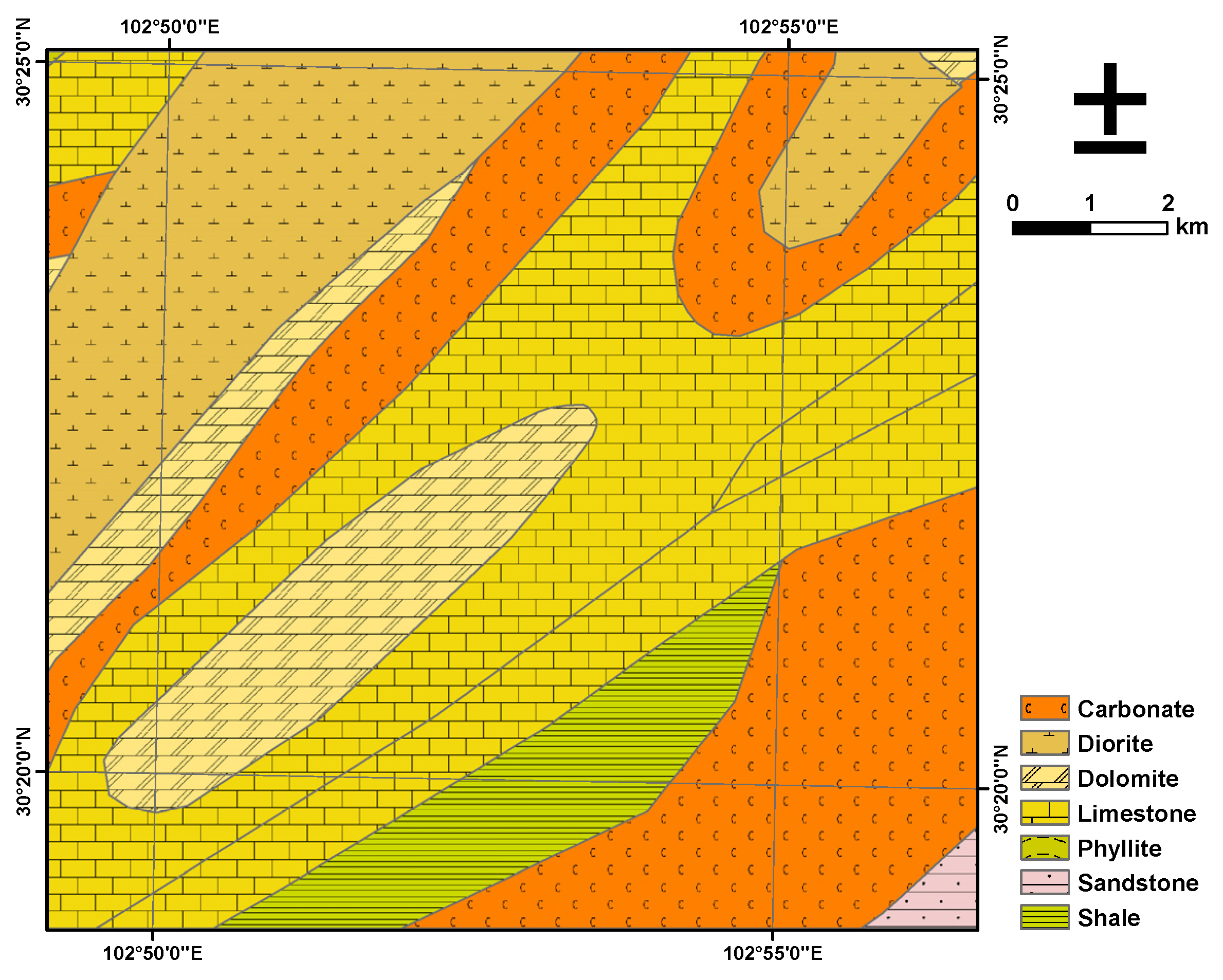
The epicenter of the 2013 6.6 Lushan earthquake is located at the southern segment of the Longmenshan fault zone, on the eastern margin of the Tibetan Plateau [36,37]. The study area was selected as a rectangular section with high concentrations of coseismic landslides (Figure 1). The study area is located about 12 km northwest of the epicenter and lies on the border of two earthquake-hit counties, i.e., Baoxing County and Lushan County in Sichuan Province, China, covering 138 km2 (Figure 1). The study area is characterized by deeply incised valleys and high mountains, with an elevation ranging from 1013 to 3308 m above sea level (Figure 1). Exposures of the geological units encompass ages ranging from the Sinian to the Triassic, incorporating a diverse range of formations such as carbonate, diorite, dolomite, limestone, phyllite, sandstone, and shale (Figure 2).
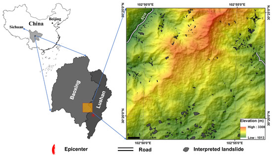
Figure 1.
Location of the study area and the interpreted landslides.
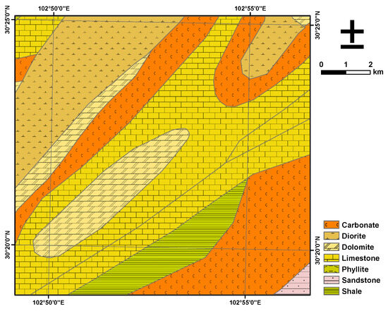
Figure 2.
Map depicting the geological units of the study area.
There have been 17 earthquakes with magnitudes ≥ 4.7 in the history of the Lushan earthquake zone [38]. Strong tectonic activity provides favorable conditions that make the region prone to landslides. The 2013 Lushan earthquake has triggered thousands of landslides [39]. An inventory of 308 coseismic landslides was compiled by making comparisons between pre-earthquake satellite images and post-earthquake aerial photographs in the study area. The cumulative area of these interpreted landslides spans 5 km2.
3. Methodology
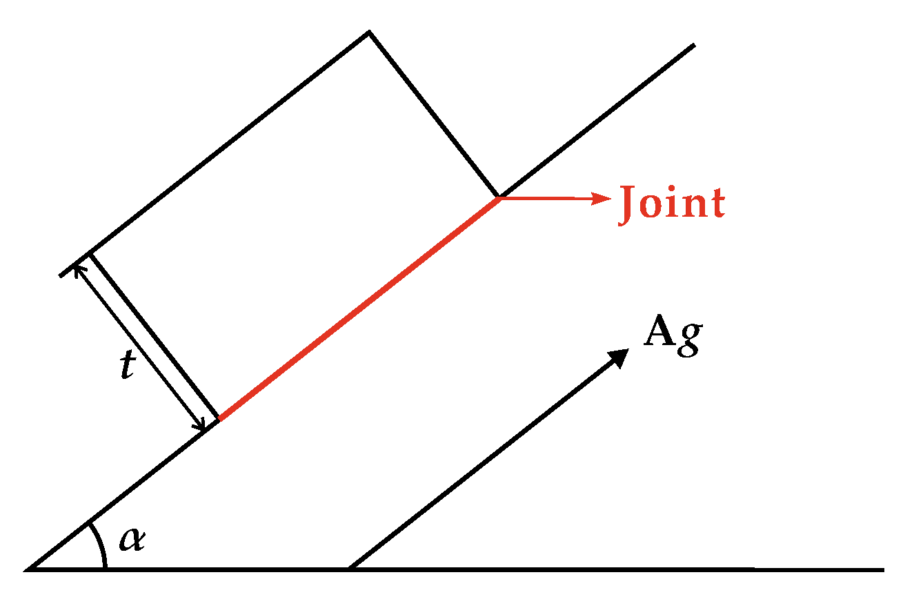
In 1965, Newmark [8] proposed an infinite slope model for the assessment of the coseismic stability of slopes. The Newmark method [8] simulates a landslide as a rigid friction block situated on an inclined plane with a predetermined critical acceleration (Figure 3). It computes the cumulative permanent displacement of the block in relation to its base, considering the impact of earthquake acceleration–time history [18,19]. The permanent displacement is a valuable index for evaluating the dynamic performance of slopes.
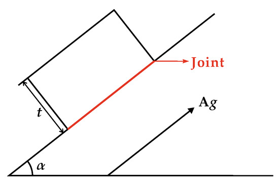
Figure 3.
Conceptual sliding-block model of Newmark analysis (adapted from Newmark [8] and Zang et al. [31]). is the angle of the slope, is the thickness of the failure rock block, is a constant, and g is the acceleration due to the Earth’s gravity.
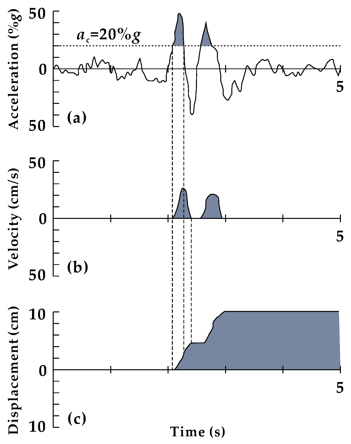
Once an acceleration–time history has been selected, segments of the record surpassing the critical acceleration (Figure 4a) are integrated once to establish a velocity profile (Figure 4b). Subsequently, the velocity–time history undergoes a second integration to yield the cumulative displacement of the block (Figure 4c) [18,19,31].
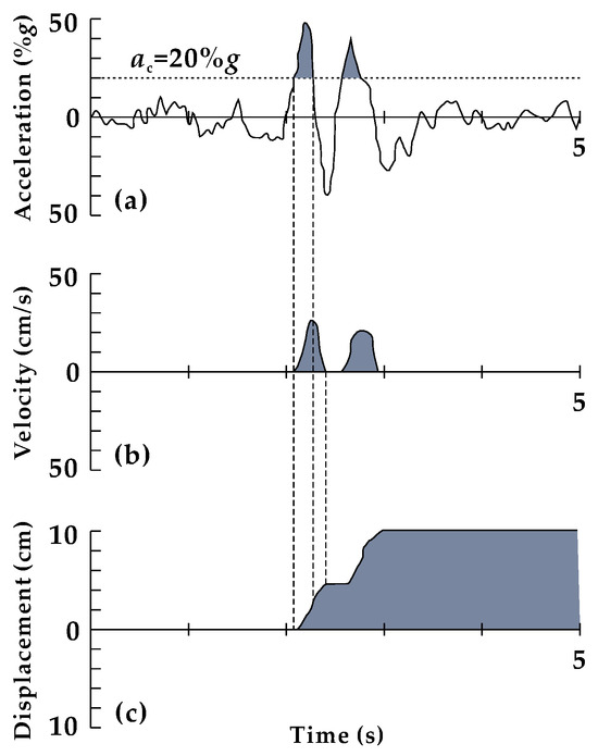
Figure 4.
Illustration of the algorithm employed in Newmark analysis (adapted from Jibson et al. [18,19]). is the critical acceleration in terms of g. (a) The acceleration–time history of earthquake with a critical acceleration (indicated by the horizontal dashed line) of 20% g superimposed. The color area represents segments of the record that exceed the critical acceleration; (b) The velocity–time history of the block. The color area stands the velocity of the block, derived from a single integration of the acceleration–time history corresponding to portions exceeding the critical acceleration; (c) The displacement–time history of the block. The color area denotes the cumulative displacement of the block, derived from the double integration of the acceleration–time history corresponding to portions exceeding the critical acceleration.
From Figure 4, we can see that critical acceleration provides a base for predicting the cumulative permanent displacement of a slope. Newmark [8] showed that the critical acceleration of a potential landslide block can be expressed as a simple function of the static factor of safety and the geometry of the slope [18,19]:
where is the critical acceleration in terms of g, is the static factor of safety, and is the angle from the horizontal at which the center of the slide block moves when displacement first occurs [18,19]. In instances of a planar slip surface parallel to the slope, it is typically noted that this angle closely approximates the slope angle.
Natural rock slopes are often cut by a group of shallow unloading joints due to valley incisions, forming an unloading zone on the surface of the slopes [24,25]. Slopes behave as collapsing and sliding failures of shallow unloading joints under intense seismic activity, with approximately 90% of coseismic landslides manifesting as shallow falls and slides [26,27,28,29]. The seismic shaking commonly triggers the activation of unstable rock blocks along rock joints (Figure 3). Therefore, the static factor of safety is related to the shear strength of these rock joints.
Zang et al. [31] derived the static factor of safety of a slope based on the Barton [32] shear strength criterion for rock joints in another study:
where is the peak shear strength of the rock joint, is the unit weight of the rock mass, is the thickness of the failure rock block, is the effective normal stress, is the joint roughness coefficient in the in situ scale, is the joint wall compressive strength in the in situ scale, and is the basic friction angle.
Considering the impact of joint size, the and can be defined as [40]:
where the adopted nomenclature includes (0) and () to represent values corresponding to the laboratory scale and the in situ scale, respectively.
It is impractical to conduct a rigorous Newmark method during the regional analysis. Therefore, researchers have proposed different empirical regressions to estimate Newmark displacement as a function of the critical acceleration and ground motion parameters [14,41,42,43,44,45]. In this study, we chose a vector model developed according to more than 2000 strong motion records [44]:
where is the predicted Newmark displacement, is the peak ground acceleration, and is the moment magnitude. is in centimeters, and and are in units of g.
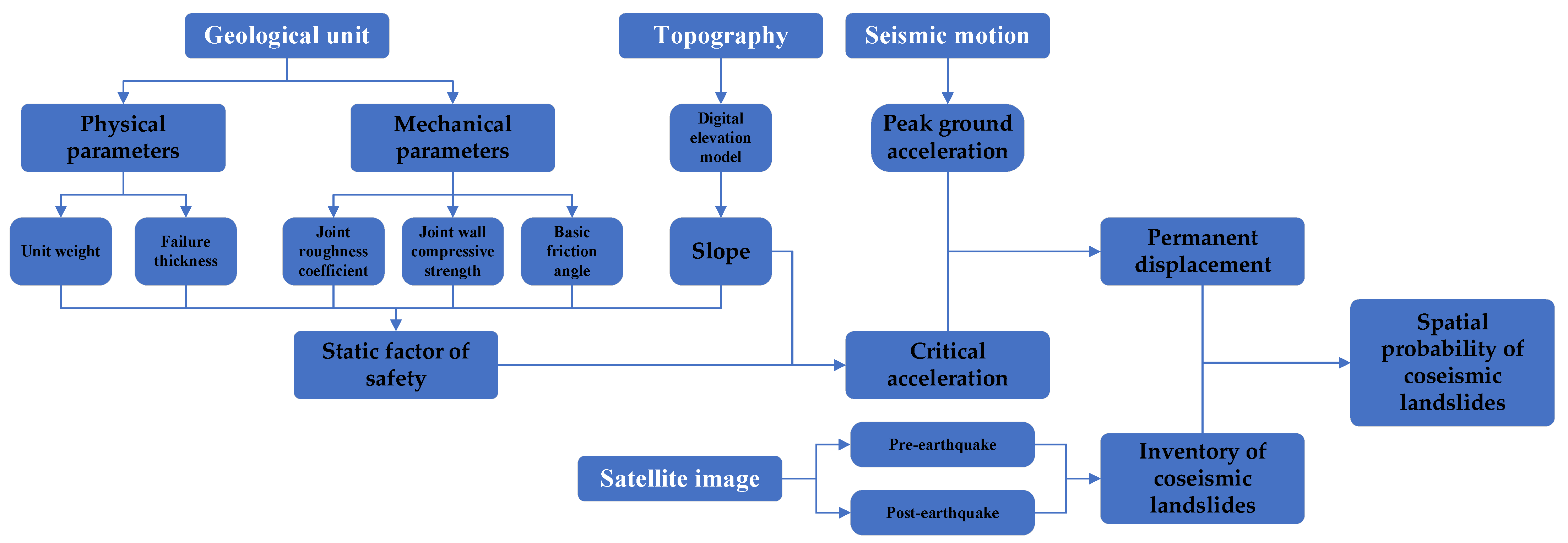
Figure 5 is a flowchart showing the sequential steps of the spatial evaluation of coseismic landslides. After calculating the Newmark displacement, the predicted displacement was then compared with an inventory of landslides induced by the Lushan earthquake, employing the certainty factor model (CFM) for mapping the spatial distribution of coseismic landslide hazards [46]. The CFM, an inexact reasoning model, initially developed by Shortliffe and Buchanan [46] and refined by Heckerman [47], serves to examine the correlation between the predicted displacement and the occurrence of landslides. Within the CFM framework, the certainty factor (CF) quantifies the net confidence in a hypothesis based on the evidence [47], ranging from −1 to 1. A CF of −1 indicates a complete lack of confidence, whereas a CF of 1 signifies absolute confidence. Values exceeding zero lean towards supporting the hypothesis, while those below zero lean towards supporting its negation. The probabilistic interpretation of CF can be articulated as follows [47]:
where CF stands for the certainty factor, represents the posterior probability denoting the conditional probability for a posterior hypothesis based on evidence, and denotes the prior probability in the absence of any evidence. For the spatial evaluation of coseismic landslides, was defined as the ratio of the landslide area within a specific displacement area, and was defined as the proportion of the landslide area within the entire study area [31]. Accordingly, CF values reflected the confidence level regarding the occurrence of coseismic landslides. Positive values indicated an increased confidence in slope failure, whereas negative values indicated a leaning towards its negation [31].

Figure 5.
Flowchart depicting the sequential steps involved in the hazard mapping procedure.
4. Mapping of Coseismic Landslide Hazard
The datasets, encompassing geological units, peak ground acceleration (PGA), and a high-resolution digital elevation model (DEM) of topography, were converted into raster format with a grid spacing of 30 m. In this section, each step involved in the mapping of coseismic landslide hazards is discussed in detail.
4.1. Static Factor of Safety Map
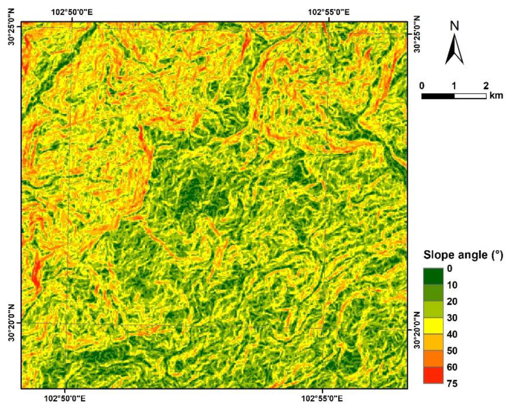
We selected a 30 m DEM to produce a slope map (Figure 6) by applying a basic slope algorithm, where the slope was identified as the steepest downhill descent among adjacent cells [48]. The derived slopes ranged from 0° to 75°. The northwestern and northeastern portions of the study area are high mountains and deeply incised valleys with slopes greater than 50°, and the central and southeastern parts of the area are relatively flat (Figure 6).
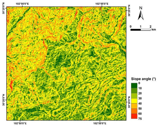
Figure 6.
Topographic slope map generated from the DEM of the study area.
We assigned physical and mechanical parameters to the rock types using a digital geological map (Figure 2). The map was rasterized at a 30 m grid spacing for the following calculation after the parameter assignment. Studies have shown that and strongly depend on lithology [49,50,51,52,53,54,55,56,57,58,59,60,61,62,63,64,65,66]. The values of and assigned to each rock type were estimated based on test data from the references listed in Table 1. These values were obtained from laboratory tests with a sample length of = 100 mm. As we used a projected coordinate system for regional analysis and the grid spacing was 30 m, the engineering dimension, , in a grid cell was equal to 30 m/cosα. We can calculate and by substituting , , , and into Equations (3) and (4), respectively. The spatial distribution of and are shown in Figure 7a,b, respectively. Other parameters such as and are listed in Table 1.

Table 1.
Shear strengths assigned to rock types in the study area.
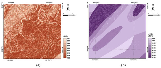
Figure 7.
Map showing shear strength components assigned to geological formations in the study area. (a) component of shear strength; (b) component of shear strength.
For simplicity, the thickness () of the rock block in failure (Figure 3) was established at 3 m, based on field investigations of typical slope failures resulting from the Lushan earthquake. We produced a map of the static factor of safety by integrating data layers of , , , , and in Equation (2). The calculated static factors of safety varied between 0.2 to 133.8. Grid cells displaying static factors of safety below 1 suggested static instability in the slopes, but this did not necessarily imply that they were undergoing sliding under seismic shaking [31]. However, according to Equation (1), to prevent obtaining a negative critical acceleration value, we assigned a minimal static factor of safety of 1.01 to these cells. Keefer [3] showed that the minimum slope angle for earthquake-induced landslides was 5°. In addition, the calculated static factors of safety for the cells with a slope angle of less than 5° were very high, and these cells did not contribute significantly to the statistical analysis due to their limited sample size [18,19]. Therefore, slopes with inclinations less than 5° were excluded from the analysis. The revised static factors of safety now fall within the range of 1 to 10.4, as depicted in Figure 8. Statically unstable slopes, characterized by a static factor of safety below 1.2, are mainly distributed in the northwestern, northeastern, and southeastern parts of the study area, as illustrated in Figure 8.
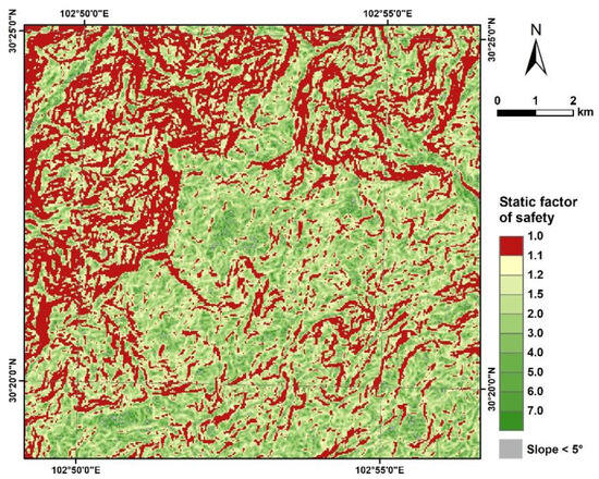
Figure 8.
Map depicting the static factor of safety across the study area.
4.2. Critical Acceleration Map
After the adjustment of the static factors of safety, we produced a map of critical acceleration using Equation (1) to integrate the slope angle with the static factors of safety (Figure 9). The critical acceleration represents the intrinsic properties of slopes independent of any shaking scenario; thus, the critical acceleration map serves as an indicator of coseismic landslide susceptibility [18,19]. A smaller value of critical acceleration denotes the lower intensity of shaking needed to overcome the stability of the slope. Therefore, coseismic sliding is more likely to develop on the slope. Figure 9 shows that the dynamically unstable slopes with a critical acceleration of less than 0.3 g are mainly distributed in the northwestern part of the study area, and only a small portion is present in the southern part of the study area.
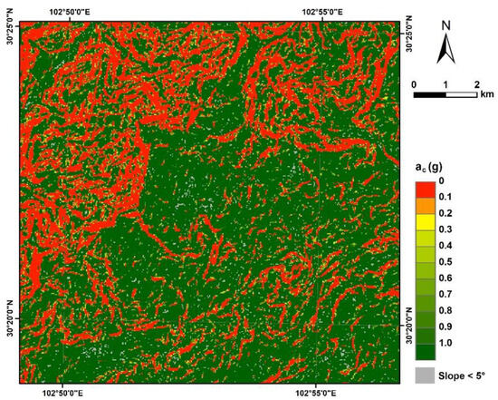
Figure 9.
Map illustrating critical accelerations across the study area.
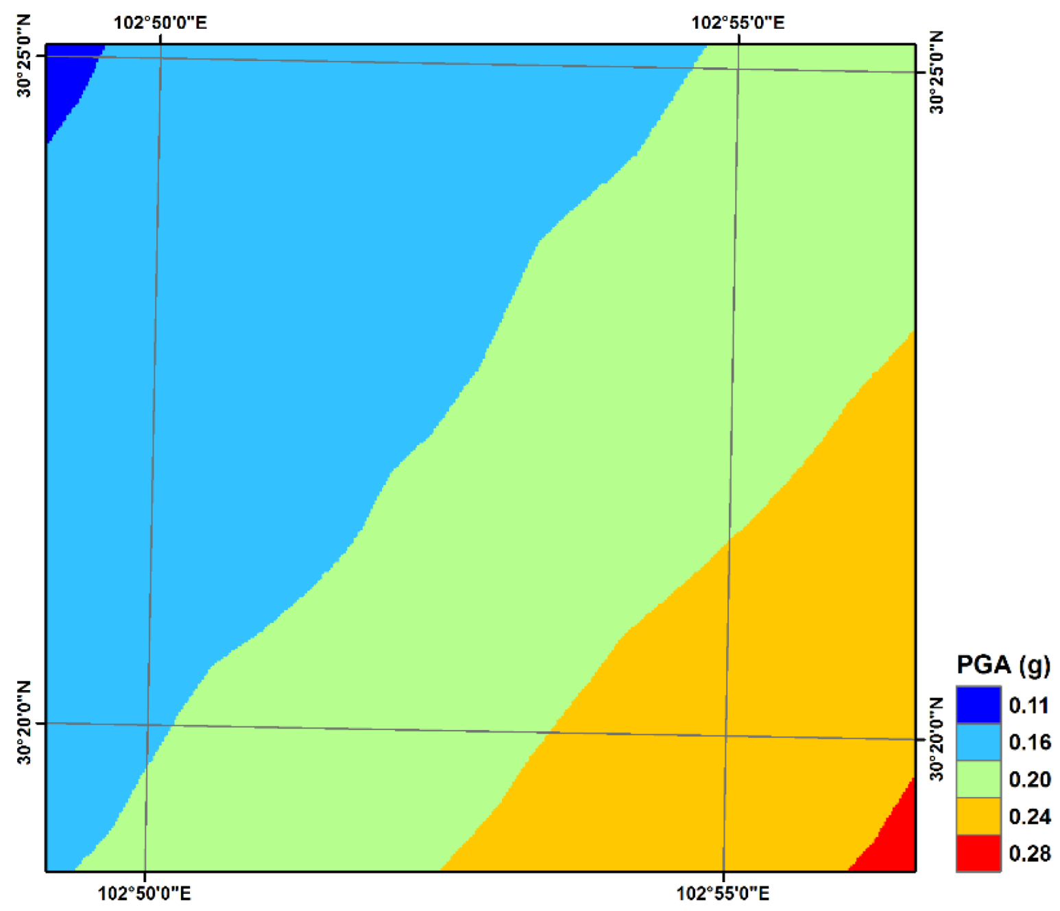
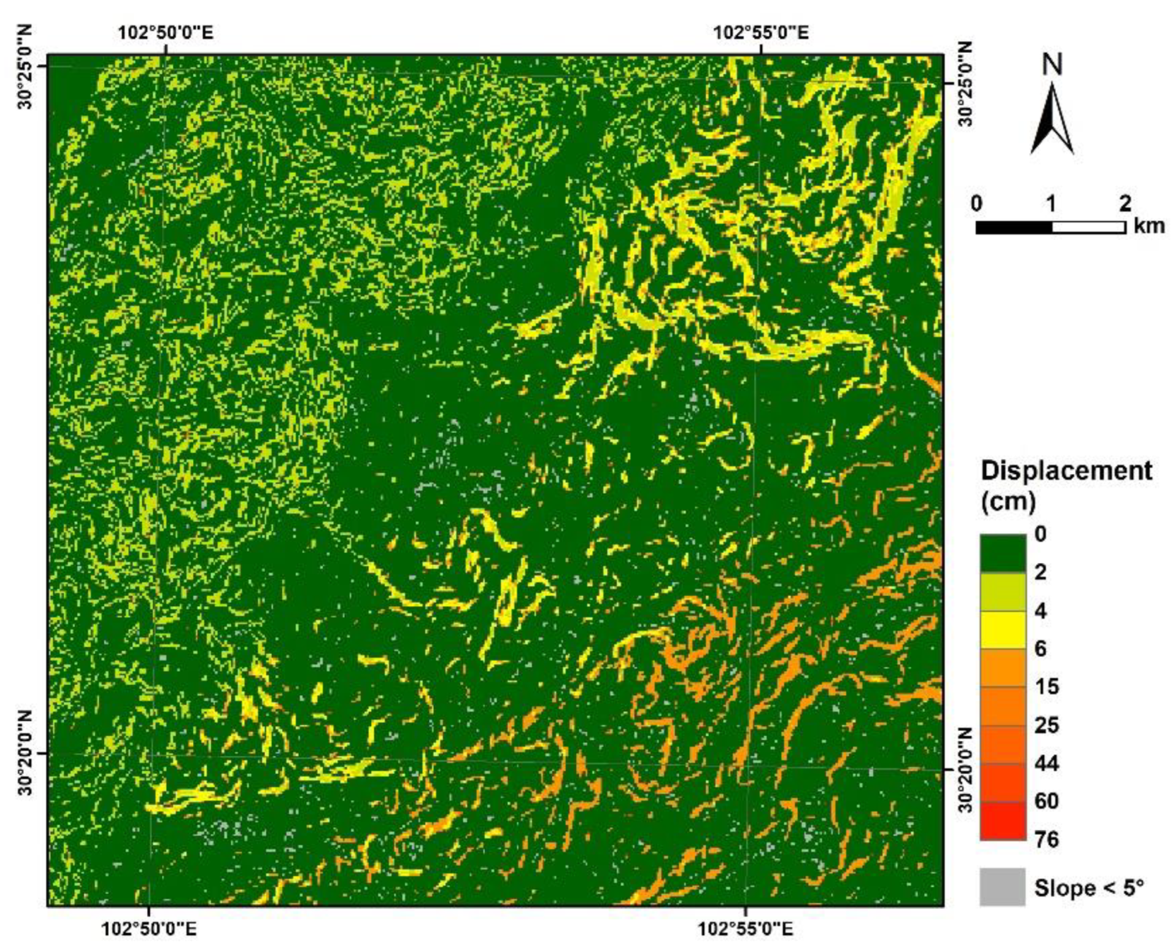
4.3. Predicted Displacement Map
We downloaded the contour map depicting the PGA in the study area (Figure 10) from the United States Geological Survey. The Newmark displacement for each cell was computed using Equation (5), integrating the respective grid values of critical acceleration, PGA, and moment magnitude. The resulting predicted displacements range from 0 to 76 cm (Figure 11). Slopes with a predicted displacement ranging between 0 cm and 4 cm are distributed in the northwestern portion of the study area, slopes with a predicted displacement ranging between 4 cm and 6 cm are distributed in the middle portion of the study area, slopes with a predicted displacement ranging between 6 cm and 15 cm are scattered in the area with a displacement between 4 cm and 6 cm, and slopes with a predicted displacement greater than 15 cm are only distributed in the southeastern portion of the study area. According to the statistical sizes of the areas, displacements less than 4 cm occupy 90.5% of the study area, displacements between 4 cm and 6 cm occupy 5.5% of the study area, and displacements between 6 cm and 15 cm occupy 3.6% of the study area, with displacements exceeding 15 cm constituting a very small area.
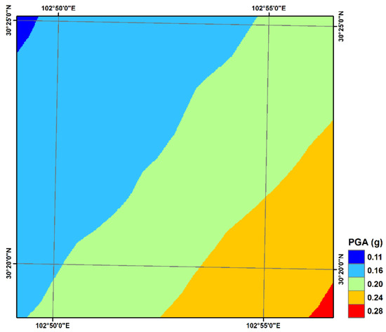
Figure 10.
Contour map illustrating peak ground acceleration (PGA). PGA values shown are in g.

Figure 11.
Map illustrating predicted displacements within the study area.
4.4. Coseismic Landslide Hazard Map
Jibson et al. [18,19] showed that Newmark displacements serve as an indicator of the coseismic performance of slopes but do not align directly with observable slope movements in the field. Consequently, a comparison of predicted displacements with an inventory of landslides induced by earthquakes was necessary to establish a predictive scenario for coseismic landslide hazards. We employed Equation (6) to generate a coseismic landslide hazard map, expressed in terms of CFs.
The Newmark displacement cells, each 1 cm, were grouped into bins. All cells with displacements between 0 cm and 1 cm were grouped into the first bin, those between 1 cm and 2 cm into the second bin, and so forth [18,19]. We grouped the predicted displacements into 75 bins. For each bin, we calculated the proportion of cells occupied by landslide areas. This proportion represents the posterior probability of the bin according to Equation (6). The proportion of the entire landslide area within the entire study area was calculated to obtain the prior probability, which was the same in each bin. Using Equation (6), we computed the values of CF by combining the corresponding posterior and prior probabilities. The calculated CFs ranged from −1 to 0.99. The CFM provides a necessary linkage between the Newmark displacements and confidence levels of coseismic landslide occurrence in the study area. We produced a coseismic landslide hazard map for the ground-shaking scenario of the Lushan earthquake based on the values of CF, as shown in Figure 12. The inventory of landslides triggered by the Lushan earthquake illustrates the fit of the predicted confidence levels of coseismic landslides.
Figure 12.
Map showing confidence levels of coseismic landslides. Confidence levels are represented by CF values.
5. Discussion
The predicted displacement refers to the cumulative sliding displacement of slopes for a specific acceleration history. As depicted in Figure 11, these predicted displacements range from 0 to 76 cm. The analysis of the statistical size of each displacement area indicates that 90.5% of the study area experiences displacements less than 4 cm, and 99.6% of the study area experiences displacements less than 15 cm. Only a very small area observes displacements greater than 15 cm. Jibson et al. [18,19] suggested that shallow, disrupted rock falls and rock slides in relatively brittle, poorly cemented sediments tend to collapse at small displacements. Thus, the study area demonstrates higher susceptibility to shallow falls and slides. According to high-resolution aerial photographs and field investigations, most landslides triggered by the Lushan earthquake were rock falls and relatively shallow, disrupted slides, typically 1–5 m in depth [29,39,68]. Therefore, the proposed model is particularly useful for predicting the spatial distribution of the typical coseismic landslides in the study area.
Predicted displacements do not accurately reflect the actual slope movement in the field. Instead, modeled displacements serve as an indicator that can be correlated with field performance [18,19]. By using a function that incorporates Newmark displacement and CF, the confidence levels of slope failure in the field can be estimated, and the spatial variation in coseismic landslides can be predicted under any set of ground-shaking conditions [31]. The number of Newmark displacement cells per 1 cm was uneven. To obtain a more reasonable regression curve correlating the predicted displacement and CF, we grouped these cells into bins based on quantile statistics. The breakpoints were set at 0, 2, 4, 6, 15, 25, 44, 60, and 76, ensuring an equal number of cells in each bin. For each bin, the proportion of cells in landslide areas was calculated, and the CF value of Newmark displacement was plotted as a dot. To fit the data, a modified Weibull [69] curve proposed by Zang et al. [31] was employed, with the following functional form:
where CF is the certainty factor, represents the maximum CF value, stands for the predicted displacement, and and are the regression constants. The regression curve derived from the Lushan data is as follows:
The data fit the curve well with an R-squared value of 92%. The CF value serves as a direct indicator for predicting the confidence level of slope failure based on Newmark displacement. Figure 13 shows that the CF value increases monotonically with increasing Newmark displacement. The CF value increases rapidly in the first 10 cm of Newmark displacement, followed by a sudden plateau after the 15 cm range, stabilizing around a CF value of approximately 0.25.

Figure 13.
CF as a function of Newmark displacement. Each dot represents the CF value for a specific Newmark displacement bin, while the red line illustrates the fitting curve of the data using a modified Weibull function.
Equation (8) mirrors the form of our previously published equation [31]. However, the equation proposed in this study has different regression constants owing to different data. After calibration, both the curve and its corresponding equation can be applied to any ground-shaking conditions. This allows the prediction of the slope failure’s confidence level, based on the predicted Newmark displacement [18,19]. However, a problem exposed by the earlier study should be noted. The maximum CF value is equal to , not , as indicated by Zang et al. [31]. The values of , , and in Equation (8) may vary in other regions if the lithology, topography, and ground motion conditions significantly differ from those observed in the study area. Additionally, the shape of the fitting curve in Figure 13 might vary in regions where different types of slope failures are predominant. If rock falls and rock slides in more brittle materials were prevalent, the fitting curve may be steeper and could flatten at a lower maximum displacement value [18,19,31]. The seismogenic fault responsible for the 2014 Ludian earthquake is the Baogunao–Xiaohe fault, identified as a left-lateral strike–slip fault [33]. In the case of the 2013 Lushan earthquake, the seismogenic fault is a blind reverse fault [35]. Upon comparing our previous studies [31], we observed that, in contrast to the Ludian earthquake, the predicted displacements caused by the Lushan earthquake exhibit a faster convergence in the fitting curve, with smaller displacement extremes. This suggests that when the seismogenic fault is a reverse fault, slope failures in the seismic region predominantly manifest as brittle fractures. Conversely, if the seismogenic fault is a strike–slip fault, the resulting landslides primarily occur in more compliant materials within the seismic region.
Figure 9 shows the distribution of critical acceleration within the study area. Critical acceleration describes the seismic susceptibility of a slope. Newmark [8] showed that the critical acceleration depends on the static factor of safety and the slope angle (Equation (1)). Comparing Figure 6 with Figure 8 and Figure 9, respectively, we found that the modeling procedure is heavily slope-driven, which is consistent with the findings from Jibson et al. [18,19]. However, in comparing Figure 11 with Figure 10, we observed that the distribution pattern of Newmark displacements bears a resemblance to that of PGA. Areas with displacements between 2 and 4 cm, 4 and 6 cm, and 6 and 15 cm are distributed in bands in the study area, indicating the dominant role of seismic ground motion in triggering coseismic landslides during the Lushan earthquake.
In Section 3, it was mentioned that during seismic activity, unstable rock blocks tend to slide along shallow unloading joints. The static factor of safety is closely related to the shear strength of these rock joints. The conventional Newmark analysis traditionally describes the shear strength of rocks using Coulomb’s constants, such as friction angle and cohesion, but these values vary significantly between laboratory conditions with high normal stress and field conditions with low normal stress [32]. Additionally, these values are also dependent on the scale of the analysis [63]. To address these challenges, we introduced the Barton model into the Newmark analysis [31]. This model enables us to predict the shear strength of rock joints and reduce the variability associated with Coulomb’s constants. Furthermore, we accounted for scale effects to prevent overestimating the shear strength of geological units in regional analysis by using Equations (3) and (4). A conventional Newmark analysis was conducted using assigned strengths like friction angle and cohesion, outlined in Table 1. The predicted displacements obtained through the conventional Newmark method ranged from 0 to 78 cm, whereas the proposed method yielded values ranging from 0 to 76 cm. Subsequently, the calculation of the CF using the conventional Newmark analysis produced a range of −1 to 0.74, while the proposed method resulted in a range of −1 to 0.99. To evaluate the performance of the two methods, we utilized the area under the curve (AUC) analysis. The AUC plot illustrates the cumulative area of CFs within each interval of calculated values, representing the proportion of the total study area (x-axis), and the proportion of cumulative landslides falling within those CFs (y-axis) [70]. An AUC value of 0.5 suggests a performance equal to random guessing, while a value of 1 indicates perfect performance [70]. Figure 14 depicts the results of the AUC analysis for both methods, with a calculated value of 0.57 for the proposed method and 0.53 for the conventional Newmark method. Therefore, the introduced method yields improved results compared to the conventional Newmark analysis.
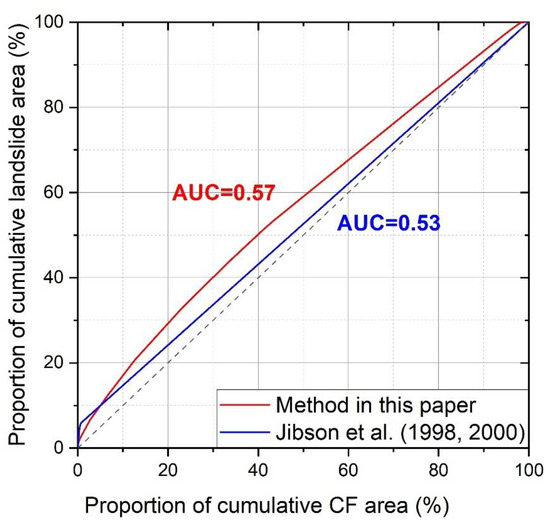
Figure 14.
Plots of the area under the curve (AUC) for a comparison between the proposed method and the conventional Newmark method [18,19]. The dot line represents an AUC value of 0.5.
However, it is noteworthy that both methods yield relatively small AUC values. This outcome can be attributed to the coseismic landslide interpretation data employed in the analysis. As is well known, landslides can be categorized into three distinct areas: the source area, the transport area, and the deposition area. The interpretation data utilized for the calculations encompass all three areas. The initiation of landslides occurs in the source area, while the deposition area is where the landslide material comes to rest. The source area is typically characterized by steep slopes, leading to relatively large Newmark displacements that align with the model’s predictions. Conversely, the deposition area tends to exhibit flatter terrain with smaller slopes, resulting in relatively smaller Newmark displacements. Nevertheless, following the occurrence of a landslide, a substantial amount of material accumulates in the deposition area. Consequently, a significant portion of the landslide area in the interpretation data falls within regions associated with smaller Newmark displacements. This leads to deviations in the predictive outcomes of the model. To achieve more accurate results, it is crucial to precisely delineate the source area of coseismic landslides and employ it as the primary input for hazard assessment. This particular aspect demands significant attention in future evaluations of coseismic landslide hazards. Furthermore, since the proposed method concentrates on assessing the stability of unloading joints based on strength parameters like the joint roughness coefficient and joint wall compressive strength during predictions, its applicability is limited to spatial assessments of rock landslide hazards. The calibrated method proves most effective in predicting the spatial distribution of relatively shallow, disrupted slides and falls in rock and debris. However, it is likely to provide less precise predictions for the distribution of deeper, coherent landslides [18,19].
6. Conclusions
This study presents a recalibration of a pioneering method designed to assess coseismic landslide hazards triggered by the 2013 Lushan earthquake. The method incorporates the roughness of potential sliding surfaces on the inner slope. The primary findings are outlined as follows:
- (1)
- The landslides induced by the 2013 Lushan earthquake are primarily concentrated in deeply incised valley regions, consisting mainly of shallow, disrupted rock falls, and rock slides.
- (2)
- For reverse seismogenic faults, slopes within the seismic region predominantly display brittle coseismic fractures. In contrast, strike–slip seismogenic faults tend to result in complaint coseismic fractures on slopes.
- (3)
- The integration of Newmark analysis with Barton’s shear strength criterion proves to be practically useful in evaluating regional coseismic landslide hazards. Moreover, the improved method demonstrates higher reliability when compared to the conventional Newmark approach, thereby contributing to the overall sustainability and resilience of communities facing such geological challenges.
Author Contributions
Conceptualization, M.Z. and S.Q.; methodology, G.L. and M.Z.; validation, T.L.; formal analysis, G.L., M.Z. and T.L.; investigation, M.Z.; resources, M.Z.; data curation, M.Z.; writing—original draft preparation, G.L. and M.Z.; writing—review and editing, M.Z., S.Q. and G.Y.; project administration, S.Q. and J.B.; funding acquisition, M.Z., S.Q. and G.Y. All authors have read and agreed to the published version of the manuscript.
Funding
This research was funded by the National Natural Science Foundation of China (grant nos. 41825018, 42207215, and 42277164).
Institutional Review Board Statement
Not applicable.
Informed Consent Statement
Not applicable.
Data Availability Statement
Data will be made available on request.
Acknowledgments
The authors thank the National Natural Science Foundation of China (grant nos. 41825018, 42207215, and 42277164). We appreciate the insightful comments from the reviewing experts and academic editor, which significantly enhanced the quality of this manuscript.
Conflicts of Interest
The authors declare no conflict of interest.
References
- Mao, Y.; Chen, L.; Nanehkaran, Y.A.; Azarafza, M.; Derakhshani, R. Fuzzy-Based Intelligent Model for Rapid Rock Slope Stability Analysis Using Qslope. Water 2023, 15, 2949. [Google Scholar] [CrossRef]
- Tao, Z.; Wang, Y.; Zhu, C.; Xu, H.; Li, G.; He, M. Mechanical Evolution of Constant Resistance and Large Deformation Anchor Cables and Their Application in Landslide Monitoring. Bull. Eng. Geol. Environ. 2019, 78, 4787–4803. [Google Scholar] [CrossRef]
- Keefer, D.K. Landslides Caused by Earthquakes. Geol. Soc. Am. Bull. GSA Bull. 1984, 95, 406–421. [Google Scholar] [CrossRef]
- Terzaghi, K. Mechanism of Landslides. In Application of Geology to Engineering Practice; Paige, S., Ed.; Geological Society of America: New York, NY, USA, 1950; pp. 83–123. ISBN 0-8137-4301-X. [Google Scholar]
- Clough, R.W.; Chopra, A.K. Earthquake Stress Analysis in Earth Dams. J. Eng. Mech. Div. 1966, 92, 197–212. [Google Scholar] [CrossRef]
- Yuan, C.; Li, Q.; Nie, W.; Ye, C. A Depth Information-Based Method to Enhance Rainfall-Induced Landslide Deformation Area Identification. Measurement 2023, 219, 113288. [Google Scholar] [CrossRef]
- Zhang, X.; Zhu, C.; He, M.; Dong, M.; Zhang, G.; Zhang, F. Failure Mechanism and Long Short-Term Memory Neural Network Model for Landslide Risk Prediction. Remote Sens. 2022, 14, 166. [Google Scholar] [CrossRef]
- Newmark, N.M. Effects of Earthquakes on Dams and Embankments. Géotechnique 1965, 15, 139–160. [Google Scholar] [CrossRef]
- Jibson, R.W. Methods for Assessing the Stability of Slopes during Earthquakes—A Retrospective. Eng. Geol. 2011, 122, 43–50. [Google Scholar] [CrossRef]
- Makdisi, F.I.; Seed, H.B. Simplified Procedure for Estimating Dam and Embankment Earthquake-Induced Deformations. J. Geotech. Eng. Div. 1978, 104, 849–867. [Google Scholar] [CrossRef]
- Bray, J.D.; Rathje, E.M. Earthquake-Induced Displacements of Solid-Waste Landfills. J. Geotech. Geoenviron. Eng. 1998, 124, 242–253. [Google Scholar] [CrossRef]
- Rathje, E.M.; Bray, J.D. An Examination of Simplified Earthquake-Induced Displacement Procedures for Earth Structures. Can. Geotech. J. 1999, 36, 72–87. [Google Scholar] [CrossRef]
- Rathje, E.M.; Bray, J.D. Nonlinear Coupled Seismic Sliding Analysis of Earth Structures. J. Geotech. Geoenviron. Eng. 2000, 126, 1002–1014. [Google Scholar] [CrossRef]
- Bray, J.D.; Travasarou, T. Simplified Procedure for Estimating Earthquake-Induced Deviatoric Slope Displacements. J. Geotech. Geoenviron. Eng. 2007, 133, 381–392. [Google Scholar] [CrossRef]
- Rathje, E.M.; Antonakos, G. A Unified Model for Predicting Earthquake-Induced Sliding Displacements of Rigid and Flexible Slopes. Eng. Geol. 2011, 122, 51–60. [Google Scholar] [CrossRef]
- Zhang, Y.; Xiang, C.; Chen, Y.; Cheng, Q.; Xiao, L.; Yu, P.; Chang, Z. Permanent Displacement Models of Earthquake-Induced Landslides Considering near-Fault Pulse-like Ground Motions. J. Mt. Sci. 2019, 16, 1244–1257. [Google Scholar] [CrossRef]
- Zhang, Y.; Xiang, C.; Yu, P.; Zhao, L.; Zhao, J.X.; Fu, H. Investigation of Permanent Displacements of Near-Fault Seismic Slopes by a General Sliding Block Model. Landslides 2022, 19, 187–197. [Google Scholar] [CrossRef]
- Jibson, R.W.; Harp, E.L.; Michael, J.A. A Method for Producing Digital Probabilistic Seismic Landslide Hazard Maps; an Example from the Los Angeles, California, Area. Open-File Rep. 1998, 98–113. [Google Scholar] [CrossRef]
- Jibson, R.W.; Harp, E.L.; Michael, J.A. A Method for Producing Digital Probabilistic Seismic Landslide Hazard Maps. Eng. Geol. 2000, 58, 271–289. [Google Scholar] [CrossRef]
- Yuan, R.; Deng, Q.; Cunningham, D.; Han, Z.; Zhang, D.; Zhang, B. Newmark Displacement Model for Landslides Induced by the 2013 Ms 7.0 Lushan Earthquake, China. Front. Earth Sci. 2016, 10, 740–750. [Google Scholar] [CrossRef]
- Ma, S.; Xu, C. Assessment of Co-Seismic Landslide Hazard Using the Newmark Model and Statistical Analyses: A Case Study of the 2013 Lushan, China, Mw6.6 Earthquake. Nat. Hazards 2019, 96, 389–412. [Google Scholar] [CrossRef]
- Jin, K.P.; Yao, L.K.; Cheng, Q.G.; Xing, A.G. Seismic Landslides Hazard Zoning Based on the Modified Newmark Model: A Case Study from the Lushan Earthquake, China. Nat. Hazards 2019, 99, 493–509. [Google Scholar] [CrossRef]
- Ma, S.; Xu, C.; Shao, X. Spatial Prediction Strategy for Landslides Triggered by Large Earthquakes Oriented to Emergency Response, Mid-Term Resettlement and Later Reconstruction. Int. J. Disaster Risk Reduct. 2020, 43, 101362. [Google Scholar] [CrossRef]
- Gu, D. Engineering Geomechanics of Rock Mass; Science Press: Beijing, China, 1979. [Google Scholar]
- Hoek, E.; Bray, J.D. Rock Slope Engineering, 3rd ed.; Taylor & Francis: Abingdon, UK, 1981. [Google Scholar]
- Harp, E.L.; Jibson, R.W. Landslides Triggered by the 1994 Northridge, California, Earthquake. Bull. Seismol. Soc. Am. 1996, 86, S319–S332. [Google Scholar] [CrossRef]
- Khazai, B.; Sitar, N. Evaluation of Factors Controlling Earthquake-Induced Landslides Caused by Chi-Chi Earthquake and Comparison with the Northridge and Loma Prieta Events. Eng. Geol. 2004, 71, 79–95. [Google Scholar] [CrossRef]
- Dai, F.C.; Xu, C.; Yao, X.; Xu, L.; Tu, X.B.; Gong, Q.M. Spatial Distribution of Landslides Triggered by the 2008 Ms 8.0 Wenchuan Earthquake, China. J. Asian Earth Sci. 2011, 40, 883–895. [Google Scholar] [CrossRef]
- Tang, C.; Ma, G.; Chang, M.; Li, W.; Zhang, D.; Jia, T.; Zhou, Z. Landslides Triggered by the 20 April 2013 Lushan Earthquake, Sichuan Province, China. Eng. Geol. 2015, 187, 45–55. [Google Scholar] [CrossRef]
- Qi, S.; Yan, C.; Liu, C. Two Typical Types of Earthquake Triggered Landslides and Their Mechanisms. In Proceedings of the 11th International and 2nd North American Symposium on Landslides, Banff; CA, USA, 2–8 June 2011; Eberhardt, E., Froese, C., Turner, K., Leroueil, S., Eds.; CRC Press: London, UK, 2012; pp. 1819–1823. [Google Scholar]
- Zang, M.; Qi, S.; Zou, Y.; Sheng, Z.; Zamora, B.S. An Improved Method of Newmark Analysis for Mapping Hazards of Coseismic Landslides. Nat. Hazards Earth Syst. Sci. 2020, 20, 713–726. [Google Scholar] [CrossRef]
- Barton, N. Review of a New Shear-Strength Criterion for Rock Joints. Eng. Geol. 1973, 7, 287–332. [Google Scholar] [CrossRef]
- Xu, X.-W.; Jiang, G.-Y.; Yu, G.-H.; Wu, X.-Y.; Zhang, J.-G.; Li, X. Discussion on Seismogenic Fault of the Ludian Ms6.5 Earthquake and Its Tectonic Attribution. Chin. J. Geophys. 2014, 57, 3060–3068. [Google Scholar]
- Qi, S.; Xu, Q.; Lan, H.; Zhang, B.; Liu, J. Spatial Distribution Analysis of Landslides Triggered by 2008.5.12 Wenchuan Earthquake, China. Eng. Geol. 2010, 116, 95–108. [Google Scholar] [CrossRef]
- Xu, X.; Wen, X.; Han, Z.; Chen, G.; Li, C.; Zheng, W.; Zhnag, S.; Ren, Z.; Xu, C.; Tan, X.; et al. Lushan MS7.0 Earthquake: A Blind Reserve-Fault Event. Chin. Sci. Bull. 2013, 58, 3437–3443. [Google Scholar] [CrossRef]
- Han, Z.; Ren, Z.; Wang, H.; Wang, M. The Surface Rupture Signs of the Lushan “4.20” Ms 7.0 Earthquake at Longmen Township, Lushan County and Its Discussion. Seismol. Geol. 2013, 35, 388–397. [Google Scholar]
- Chen, X.L.; Yu, L.; Wang, M.M.; Lin, C.X.; Liu, C.G.; Li, J.Y. Brief Communication: Landslides Triggered by the Ms = 7.0 Lushan Earthquake, China. Nat. Hazards Earth Syst. Sci. 2014, 14, 1257–1267. [Google Scholar] [CrossRef]
- Xu, C.; Xu, X.; Zheng, W.; Wei, Z.; Tan, X.; Han, Z.; Li, C.; Liang, M.; Li, Z.; Wang, H.; et al. Landslides Triggered by the April 20, 2013 Lushan, Sichuan Province Ms 7.0 Strong Earthquake of China. Seismol. Geol. 2013, 35, 641–660. [Google Scholar]
- Xu, C.; Xu, X.; Shyu, J.B.H. Database and Spatial Distribution of Landslides Triggered by the Lushan, China Mw 6.6 Earthquake of 20 April 2013. Geomorphology 2015, 248, 77–92. [Google Scholar] [CrossRef]
- Barton, N.; Bandis, S. Effects of Block Size on the Shear Behavior of Jointed Rock. In Proceedings of the 23rd U.S Symposium on Rock Mechanics (USRMS), Berkeley, CA, USA, 25–27 August 1982; 1982; pp. 739–760. [Google Scholar]
- Ambraseys, N.N.; Menu, J.M. Earthquake-Induced Ground Displacements. Earthq. Eng. Struct. Dyn. 1988, 16, 985–1006. [Google Scholar] [CrossRef]
- Jibson, R.W. Regression Models for Estimating Coseismic Landslide Displacement. Eng. Geol. 2007, 91, 209–218. [Google Scholar] [CrossRef]
- Saygili, G.; Rathje, E.M. Empirical Predictive Models for Earthquake-Induced Sliding Displacements of Slopes. J. Geotech. Geoenviron. Eng. 2008, 134, 790–803. [Google Scholar] [CrossRef]
- Rathje, E.M.; Saygili, G. Probabilistic Assessment of Earthquake-Induced Sliding Displacements of Natural Slopes. Bull. N. Z. Soc. Earthq. Eng. 2009, 42, 18–27. [Google Scholar] [CrossRef]
- Hsieh, S.-Y.; Lee, C.-T. Empirical Estimation of the Newmark Displacement from the Arias Intensity and Critical Acceleration. Eng. Geol. 2011, 122, 34–42. [Google Scholar] [CrossRef]
- Shortliffe, E.H.; Buchanan, B.G. A Model of Inexact Reasoning in Medicine. Math. Biosci. 1975, 23, 351–379. [Google Scholar] [CrossRef]
- Heckerman, D. Probabilistic Interpretations for Mycin’s Certainty Factors. In Machine Intelligence and Pattern Recognition: Uncertainty in Artificial Intelligence; Kanal, L.N., Lemmer, J.F., Eds.; Elsevier Science Publishers B.V.: Amsterdam, The Netherlands, 1986; Volume 4, pp. 167–196. ISBN 0923-0459. [Google Scholar]
- Burrough, P.A.; McDonnell, R.A. Principles of Geographical Information Systems, 2nd ed.; Oxford University Press: Oxford, UK, 1998; ISBN 0198322663. [Google Scholar]
- Bandis, S.C.; Lumsden, A.C.; Barton, N.R. Fundamentals of Rock Joint Deformation. Int. J. Rock Mech. Min. Sci. Geomech. Abstr. 1983, 20, 249–268. [Google Scholar] [CrossRef]
- Singh, T.N.; Kainthola, A.; Venkatesh, A. Correlation Between Point Load Index and Uniaxial Compressive Strength for Different Rock Types. Rock Mech. Rock Eng. 2012, 45, 259–264. [Google Scholar] [CrossRef]
- Giusepone, F.; Da Silva, L.A.A. Hoek & Brown and Barton & Bandis Criteria Applied to a Planar Sliding at a Dolomite Mine in Gandarela Synclinal; International Society for Rock Mechanics and Rock Engineering: Goiania, Brazil, 2014. [Google Scholar]
- Yong, R.; Ye, J.; Liang, Q.-F.; Huang, M.; Du, S.-G. Estimation of the Joint Roughness Coefficient (JRC) of Rock Joints by Vector Similarity Measures. Bull. Eng. Geol. Environ. 2018, 77, 735–749. [Google Scholar] [CrossRef]
- Sirkiä, J.; Kallio, P.; Iakovlev, D.; Uotinen, L. Photogrammetric Calculation of JRC for Rock Slope Support Design. In Proceedings of the Eighth International Symposium on Ground Support in Mining and Underground Construction; Nordlund, E., Jones, T., Eitzenberger, A., Eds.; Luleå University of Technology: Luleå, Sweden, 2016; p. 13. [Google Scholar]
- Bao, H.; Zhang, G.; Lan, H.; Yan, C.; Xu, J.; Xu, W. Geometrical Heterogeneity of the Joint Roughness Coefficient Revealed by 3D Laser Scanning. Eng. Geol. 2020, 265, 105415. [Google Scholar] [CrossRef]
- Arzúa, J.; Alejano, L.R.; Clérigo, I.; Pons, B.; Méndez, F.; Prada, F. Stability Analysis of a Room & Pillar Hematite Mine and Techniques to Manage Local Instability Problems. In Proceedings of the Rock Engineering and Rock Mechanics: Structures in and on Rock Masses; Alejano, R., Perucho, Á., Olalla, C., Jiménez, R., Eds.; CRC Press: Boca Raton, FL, USA, 2014; pp. 1147–1152. [Google Scholar]
- Andrade, P.S.; Saraiva, A.A. Estimating the Joint Roughness Coefficient of Discontinuities Found in Metamorphic Rocks. Bull. Eng. Geol. Environ. 2008, 67, 425–434. [Google Scholar] [CrossRef]
- Marques, E.A.G.; Williams, D.J.; Assis, I.R.; Leão, M.F. Effects of Weathering on Characteristics of Rocks in a Subtropical Climate: Weathering Morphology, in Situ, Laboratory and Mineralogical Characterization. Environ. Earth Sci. 2017, 76, 602. [Google Scholar] [CrossRef]
- Srivastava, L.P. Probabilistic Analysis of Borehole Data for Evaluation of Engineering Properties of Rock Mass. In Proceedings of the Geotechnical Characterization and Modelling; Latha, G.M., Rao, P.R., Eds.; Springer: Singapore, 2020; pp. 503–510. [Google Scholar]
- Coulson, J.H. Shear Strength of Flat Surfaces in Rock; Cording, E.J., Ed.; American Society of Civil Engineers: Urbana, IL, USA, 1972; pp. 77–105. [Google Scholar]
- Priest, S.D. Discontinuity Analysis for Rock Engineering; Chapman & Hall: London, UK, 1993; ISBN 0-412-47600-2. [Google Scholar]
- Tang, Z.C.; Zhang, Q.Z.; Peng, J.; Jiao, Y.Y. Experimental Study on the Water-Weakening Shear Behaviors of Sandstone Joints Collected from the Middle Region of Yunnan Province, P.R. China. Eng. Geol. 2019, 258, 105161. [Google Scholar] [CrossRef]
- Tang, J.-Z.; Yang, S.-Q.; Elsworth, D.; Tao, Y. Three-Dimensional Numerical Modeling of Grain-Scale Mechanical Behavior of Sandstone Containing an Inclined Rough Joint. Rock Mech. Rock Eng. 2021, 54, 905–919. [Google Scholar] [CrossRef]
- Barton, N.; Choubey, V. The Shear Strength of Rock Joints in Theory and Practice. Rock Mech. Felsmech. Mcanique Roches 1977, 10, 1–54. [Google Scholar] [CrossRef]
- Bilgin, H.A.; Pasamehmetoğlu, A.G. Shear Behaviour of Shale Joints under Heat in Direct Shear; Barton, N., Stephansson, O., Eds.; CRC Press: Loen, Norway, 1990; pp. 179–183. [Google Scholar]
- Hashemi, S.S.; Zoback, M.D. Permeability Evolution of Fractures in Shale in the Presence of Supercritical CO2. J. Geophys. Res. Solid Earth 2021, 126, e2021JB022266. [Google Scholar] [CrossRef]
- Qu, G.; Shi, T.; Zhang, Z.; Su, J.; Wei, H.; Guo, R.; Peng, J.; Zhao, K. Characteristics Description of Shale Fracture Surface Morphology: A Case Study of Shale Samples from Barnett Shale. Processes 2022, 10, 401. [Google Scholar] [CrossRef]
- Geological Engineering Handbook Editorial Committee. Geological Engineering Handbook, 5th ed.; China Architecture & Building Press: Beijing, China, 2018. [Google Scholar]
- Xu, C.; Xu, X.; Shyu, J.B.H.; Gao, M.; Tan, X.; Ran, Y.; Zheng, W. Landslides Triggered by the 20 April 2013 Lushan, China, Mw 6.6 Earthquake from Field Investigations and Preliminary Analyses. Landslides 2015, 12, 365–385. [Google Scholar] [CrossRef]
- Weibull, W. A Statistical Theory of the Strength of Materials; Generalstabens Litografiska Anstalts Förlag: Stockholm, Sweden, 1939. [Google Scholar]
- Miles, S.B.; Keefer, D.K. Evaluation of CAMEL—Comprehensive Areal Model of Earthquake-Induced Landslides. Eng. Geol. 2009, 104, 1–15. [Google Scholar] [CrossRef]


Disclaimer/Publisher’s Note: The statements, opinions and data contained in all publications are solely those of the individual author(s) and contributor(s) and not of MDPI and/or the editor(s). MDPI and/or the editor(s) disclaim responsibility for any injury to people or property resulting from any ideas, methods, instructions or products referred to in the content. |
© 2023 by the authors. Licensee MDPI, Basel, Switzerland. This article is an open access article distributed under the terms and conditions of the Creative Commons Attribution (CC BY) license (https://creativecommons.org/licenses/by/4.0/).