Impact and Spatial Effect of Socialized Services on Agricultural Eco-Efficiency in China: Evidence from Jiangxi Province

Abstract

Agricultural eco-efficiency (AEE) is a crucial indicator of the green development of agriculture. Agricultural socialized services (AS) provide services for the agricultural production process and they promote the effective input of production factors, such as science and technology, talent, information, and capital, into the agricultural production chain, deepening the division of labor and injecting vitality into agricultural development. We measured AEE based on field research data in Jiangxi Province, China. We also constructed an endogenous switching model to explore the impact of AS on AEE. Our results show that, based on the counterfactual assumption, the AEE increased by 13.19% among farmers who adopted the services compared to those who did not. From the perspective of scale and structural differences, the larger the scale of agricultural cultivation, the stronger the impact of AS on AEE. Furthermore, a large share of cash crops was found to inhibit the impact of AS on AEE. We also investigated whether farmers in close proximity to each other affect their neighbors through knowledge dissemination and technology spillover. The extent of the impact of AS on AEE depended on distance thresholds: it was more pronounced when we increased the distance threshold. Our results suggest that the government should improve the AS system, provide more public welfare services, and appropriately subsidize AS organizations. The AS for food crops should be emphasized; however, those for cash crops should not be ignored.

1. Introduction

China’s agriculture has recently made considerable advances, using 7% of the world’s arable land to feed 20% of the world’s population, with a total grain output of 68.285 billion kilograms in 2021 [1]. But this also brought about a series of ecological and environmental problems. China uses the largest amount of chemical fertilizer in the world and the excessive application of chemical fertilizer, pesticides, and other chemicals has degraded soil fertility, caused eutrophication of water bodies, and increased agricultural carbon emissions. The traditional agricultural production model of high input, high consumption, and low efficiency is unsustainable. In response to this problem, the Chinese government has put forward a zero-growth strategy for chemical fertilizers and pesticides. The No. 1 document of the Central Government also proposes to promote the green transformation of rural production and lifestyle, sustainably reduce the application of chemical fertilizers and pesticides, strengthen the management of agricultural surface pollution, and improve the rural ecological environment in 2021 and 2022. Advancing the green transformation of agriculture means promoting the transformation of agriculture from one with a focus on production and income to one based on quality. This includes promoting resource-saving and environmentally friendly agricultural production methods. Agricultural eco-efficiency (AEE) is a measure of green agricultural development. It quantifies the efficiency of inputs and outputs in agricultural production and incorporates environmental factors into the evaluation.

Neoclassical economic growth theory holds that the driving force of economic growth originates from the increase in factor inputs and the improvement of productivity [2,3]. With the rapid development of the economy and society, there is a contradiction between economic development and the resources of the environment. It is increasingly believed that it is undesirable to develop the economy at the expense of the resource environment and that resource environment factors should be incorporated into analytical frameworks of productivity [4,5]. AEE can be understood as a measure of agricultural production efficiency that takes into account the consumption of resources and the environment, such as agricultural surface pollution. It indicates that a certain combination of production factor inputs can maximize agricultural economic output with minimal resource consumption and environmental pollution [6]. Combining the relevant literature in China and elsewhere, we found that research on AEE pertains to two aspects: measuring AEE and the factors that influence AEE. Scholars have made many achievements in evaluating AEE, measuring AEE at different scales and with different agricultural structures in the United States, South America [7,8], Asia [9,10], Europe [11], and Africa [12]. Methods of measuring AEE include data envelopment analysis (DEA), the stochastic frontier approach (SFA), the life-cycle approach, the ecological footprint approach, energy value analysis, and the ratio approach [9]. Of these, DEA and the SFA are the most commonly used. Regarding the influence factors of AEE, scholars have paid attention to the influence on AEE of factors such as AS [13], environmental regulation [14], planting structure [15], agricultural land transfer [16], rural labor force transfer [17], and population aging [18], achieving fruitful results. AS, as part of the modern industrial division of labor system, promote the effective input of production factors, such as science and technology, talent, information, and capital, into the agricultural production chain, enhancing the efficiency of agricultural production and the coordination of the industrial chain [19].

AS provide specialized services for agricultural production, acting as human capital and transmitters of knowledge and technology, to help farmers access information and new cultivation techniques; they plays a growing role in today’s agricultural production. Studies on the impact of AS on AEE focus on the following aspects. First, there are studies on the impact of AS on agricultural economic output. Some scholars have found through empirical research that the AS improve the agricultural production participation of farmers, the production scale and production mode, agricultural productivity [20], and high-quality agricultural development [21]. Some research shows that AS have a negative impact on agricultural technical efficiency and that the advantage of outsourcing services is more diversified and advanced services can be chosen, albeit at the risk of cutting corners and allowing opportunistic behavior by service providers [22]. Second, studies have considered the impact of the AS on agricultural surface pollution, showing that agricultural production services promote green growth in agriculture and that service-scale operations are an important pathway for fertilizer reduction [23,24]. AS have a significant negative impact on the application of fertilizers and pesticides by farmers and agricultural production services can promote the specialized division of labor and precision production, facilitating the reduction in chemical fertilizer [25]. AS promote fertilizer reduction by promoting the adoption of mechanized fertilizer application, expansion of the scale of farmland operations, and increase in farm household income. Third, researchers have considered the ecological impact of AS on agriculture. Zhang et al. [13] examined the impact of AS on AEE based on survey data in China. They found that the AEE was promoted by green input guidance services, soil formula fertilization services, deep plowing and deep pine services, and green pest prevention and control services.

Previous literature on the effect of AS on AEE provided a reference for our study, the contributions of which are as follows. First, most studies focus on AEE at the provincial or municipal level and pay insufficient attention to the AEE of farm households at the micro level. Farm households, as the micro-individuals of agricultural production, are important and realistic for the study of AEE. As a micro-individual of agricultural production, they are of great practical significance to studying the AEE of farm households. Second, there is simultaneous decision making between AS adoption and agricultural production behavior. We use the endogenous switching model (ESR) and counterfactual analysis can solve the problems of simultaneous decision making and self-selection and make the estimation results more scientific. Third, previous literature has paid less attention to the impact on AEE of socialized services directly related to fertilizer and pesticide inputs. Fourth, previous literature ignored the social attributes of farm households, separating them from the groups to which they belong and analyzing them separately. However, farmers interact with each other by communicating and exchanging information and their behavior when using socialized services is influenced by other farmers in close proximity. This can lead to bias in the estimation results if this spatial effect is ignored.

The goal of this paper is to investigate whether AS can have an impact on AEE. Specifically, this study involves three main goals: first, we will scientifically measure the AEE of farm households; second, we will investigate what factors are influencing farmers’ choice of AS and to what extent AS affect AEE; third, we are going to explore whether there is mutual learning among farmers and whether the adoption of AS by farmers has spatial spillover effects on the AEE of other farmers. To this end, based on research data on 711 farming households in Jiangxi Province, China, we adopted the super-efficient slack-based measure (SBM) model based on non-expected output to measure AEE. We constructed an endogenous transformation model and a spatial econometric model to empirically test the impact of AS on AEE and to provide policy suggestions for improving the construction of the AS system and promoting the green development of agriculture (Figure 1).

The rest of the paper is organized as follows. Section 2 reviews existing studies and presents our research hypotheses. Section 3 describes the methodology and data. Section 4 presents the empirical results and robustness tests. Section 5 provides a discussion and concludes.

2. Theoretical Framework

Literature Review and Research Hypotheses

Farmers, as rational subjects of microeconomic activities, seek to maximize the allocation of resources under the existing constraints. Under the combined influence of factors such as labor migration and the marketization of agricultural production, labor shortages and the separation of farm and livestock systems have emerged [26]. Farmers have shifted from applying farmyard manure and intensive cultivation to applying large quantities of chemical fertilizers in order to save labor and increase yields [27]. Under the condition of a small-farm economy, farmers naturally lack information channels to acquire and use new agricultural technologies. AS belong to the category of a professional division of labor in the agricultural field, playing the dual role of human capital and knowledge transmitter [20] and enhancing the degree of specialization in agricultural management. This professional division of labor, thus, improves production efficiency. AS have changed the traditional empirical fertilization and drug application methods and introduced new production factors through the adoption of deep fertilization technology and precision operation technology. This reduces the need for chemical and labor inputs. To maximize individual benefits, farmers are faced with the choice of producing or trading. Farmers can choose to trade through the purchase of services, the involvement of agricultural production, and the use of management activities in the external division of labor until all their own production links are gradually transferred to more AS organizations (or individuals). This effective division of labor can improve agricultural business performance. Because of biochemical technology (fertilizers, pesticides, etc.), there is an indivisible scale threshold [28]. For example, market fertilizers are generally about 50 kg per bag and small farmers often must buy the whole bag. If there is extra fertilizer and pesticide, farmers usually apply it as well to the farmland, resulting in an excessive application of fertilizers and pesticides. However, dosing and fertilizer application services provided by AS organizations can reduce waste and improve the efficiency of fertilizer application through precision applications. This leads to research hypothesis H1:

Hypothesis 1 (H1):

AS have a positive impact on AEE.

According to the new economic geography, economic individuals in close proximity to each other can drive their neighbors through knowledge dissemination and technological spillover. As such, the production behavior of farmers may be influenced by neighboring farmers and the AEE of individual farmers may be influenced by their neighbors. Farmers have strong learning and imitation behavior in terms of production decision making, which eventually manifests itself in the phenomenon of following the herd. The geographic environment, natural resources, and production methods of neighboring farmers are relatively similar; thus, the exchange cost of agricultural production factors between neighboring farmers is low. AS are intensive with regard to knowledge and technology and they have high mobility [24]. This is exhibited in the process of technology diffusion with the characteristics of geographic proximity. For the characteristics of the neighborhood network, the adoption of AS by farmers may produce driving effects, demonstration effects, imitation effects, and so on to promote the diffusion of technology. Technology diffusion generated by AS promotes the optimization of agricultural resource allocation to neighboring farmers, thus improving the AEE. As a result, research hypothesis H2 is proposed:

Hypothesis 2 (H2):

AS have a positive spatial spillover effect on AEE.

3. Methods and Data

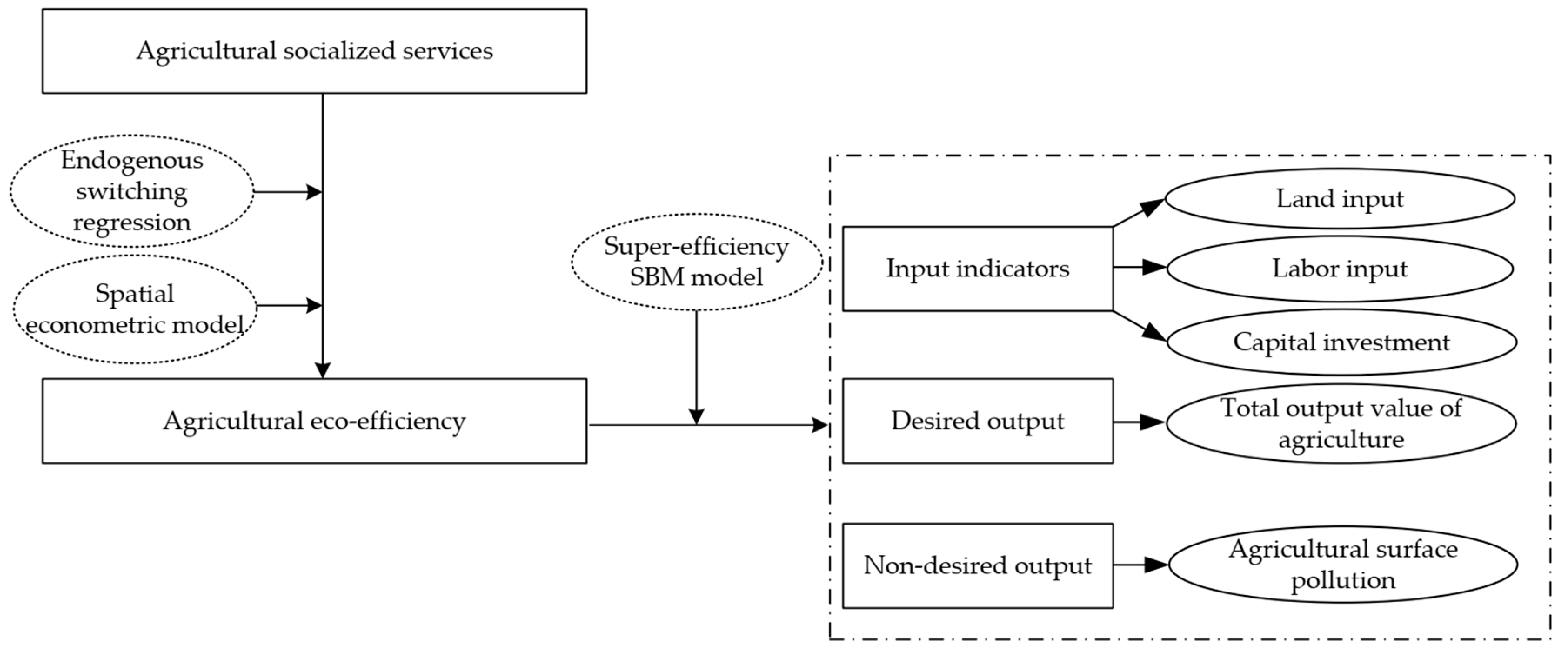
3.1. Research Methodology

3.1.1. Calculation of AEE

DEA is a non-parametric method that overcomes the influence of non-technical factors on the frontier production function and allows for the assessment of the AEE of multiple inputs and multiple outputs. In agricultural production, the input of human capital and physical capital produces not only agricultural products but also by-products of agricultural surface pollution, i.e., non-desired output. The SBM model takes into account the non-desired output in the process of production and is closer to reality. In this paper, the non-desired output super-efficiency SBM model was used to calculate the green productivity of agriculture, with the total value of agricultural output as the desired output and agricultural surface pollution as the non-desired output. The results were measured using software MaxDEA Ultra 8.22. The model settings [29,30] are as follows:

Suppose a production system has n decision units, each consisting of three input–output vectors: the input vector $X=[x_1,x_2,\cdots ,x_n]\in {\mathrm{R}}^{m\times n}$, the desired output vector $Y^g=[y_1^g,y_2^g,\cdots ,y_n^g]\in {\mathrm{R}}^{S^{1\times n}}$, and the undesired output vector $Y^b=[y_1^b,y_2^b,\cdots ,y_n^b]\in {\mathrm{R}}^{S_2\times n}$. We use m units of inputs to produce the desired output of S₁ and the undesired output of S₂. Assuming X > 0, Y^g > 0 and Y^b > 0, the production possibility set can be defined as $P=\{x,y^g,y^b|x\ge X\theta ,y^g\ge Y^g\theta ,y^b\le Y^b\theta ,\theta \ge 0\}$.

The formula for the non-expected output super-efficiency SBM model is:

$$\begin{array}{l}\\ {\rho }_{}=\min \frac{\frac{1}{m}{\displaystyle \sum _{i=1}^m\overline{x_i}/x_{i0}}}{\frac{1}{S_1+S_2}({\displaystyle \sum _{r=1}^{S_1}\overline{y_r^g}/y_{r0}^g+{\displaystyle \sum _{j=1}^{S_2}\overline{y_r^b}/y_{r0}^b}})}\\ s.t.\{\begin{array}{c}\overline{x}\ge {\displaystyle \sum _{j=1,j\ne k}^n{\theta }_j{x}_j}\\ {\overline{y}}^g\ge {\displaystyle \sum _{j=1,j\ne k}^n{\theta }_j{y}_j^g}\\ {\overline{y}}^b\ge {\displaystyle \sum _{j=1,j\ne k}^n{\theta }_j{y}_j^b}\\ \overline{x}\ge x_0,{\overline{y}}^g\le y_0^g,{\overline{y}}^b\ge y_0^b,{\overline{y}}^g\ge 0,\theta \ge 0\end{array}\end{array}$$

(1)

where $\rho$ is the efficiency value of the evaluated unit and $S=(S^{-},S^{\mathrm{g}},S^b)$ denotes the amount of slack in the inputs, desired outputs, and undesired outputs.

3.1.2. Effect of AS on AEE

Based on the aims and theoretical foundation of this paper, we considered selectivity bias caused by observable and unobservable factors, referring to Ma et al. and Zhang et al. [31,32]. The endogenous switching regression (ESR) model is used to empirically study the impact of AS on AEE. The estimation process of ESR has two stages: the first stage selects the equation to estimate the probability of farmers adopting socialized services; the second stage influences the outcome equation to estimate the impact of socialized services on farmers’ AEE.

Whether to use socialized services mainly depends on the utility generated by the services. If the utility that can be obtained after using the socialized services is $I_{1i}^{\ast }$, the utility of not using the socialized services is $I_{0i}^{\ast }$, if $I_i^{\ast }=I_{1i}^{\ast }-I_{0i}^{\ast }>0$ and farmers will choose to use them. Otherwise, they will choose not to use them. However, $I_{1i}^{\ast }$ is an unobserved variable and, in practice, it can only be observed whether farmers use AS or not. Therefore, the choice equation for the use of AS by farmers is constructed as follows:

$$I_i{}^{\ast }=\alpha X_i+{\epsilon }_i,(I_i=1,when{I}_i^{\ast }>0;I_i=0,when{I}_i^{\ast }\le 0)$$

(2)

where $I_i$ is a binary variable, $I_i=1$ denotes the use of AS by farmers and vice versa, $X_i$ denotes the relevant variables affecting the use of AS by farmers, and ${\epsilon }_i$ is a random disturbance term.

AEE is assumed to be the observable variable. Its linear regression equation is constructed with the dichotomous variable of the use of AS and estimated using the OLS method:

$$E_i=\beta {\varphi }_i+\lambda I_i+{\mu }_i$$

(3)

where $E_i$ is the value of AEE, which is calculated using the SBM model of the super-efficient non-expected output; ${\varphi }_i$ is the observed variable affecting AEE; $\beta ,\lambda$ is the coefficient to be estimated; and ${\mu }_i$ is a random interference term. For simultaneous decision making between the use of AS and agricultural production, it is assumed in the choice equation that the use of AS is exogenous. But, in fact, the use of AS is based on individual choices (such as comparative advantages formed by expected returns), which leads to the self-selection problem. The solution is to establish a joint equation and adopt an ESR model that can better overcome the endogeneity problem and effectively improve the invalid and biased estimation results [20].

This paper draws on the literature of Tesfay et al. [33] to illustrate the impact of the use of AS on AEE. The ESR model transforms Equation (3) into Equations (4a) and (4b) to model the impact effect on AEE for the use group and the non-use group, respectively:

$$E_{1i}={\beta }_1{\varphi }_{1i}+{\mu }_{1i},\mathrm{if}{I}_i=1$$

(4a)

$$E_{2i}={\beta }_2{\varphi }_{0i}+{\mu }_{2i},\mathrm{if}{I}_i=0$$

(4b)

where $E_{1i}$ in Equation (4a) and $E_{2i}$ in Equation (4b) denote the AEE in the AS use and non-use groups, respectively; ${\beta }_1,{\beta }_2$ denotes the parameter to be estimated; and ${\mu }_{1i},{\mu }_{2i}$ is a random error term. When unobservable factors simultaneously affect the use of AS and AEE, the residual terms of the choice equation and the impact effect model are correlated. That is, ${\sigma }_{1\epsilon }=\mathrm{cov}({\mu }_{1i},\epsilon )$ and ${\sigma }_{2\epsilon }=\mathrm{cov}({\mu }_{2i},\epsilon )$ denote the covariance of the error terms of the choice equation and the impact effect model, respectively. If the correlation is significant, there is indeed a simultaneous decision and a self-decision between the two decision-making behaviors. If the correlation between the two is significant, there is simultaneous decision making and self-selection between the two decision-making behaviors, which leads to biased estimation results obtained by the OLS estimation method. Therefore, the ESR model introduces the inverse Mills ratio ($\lambda$), which is calculated based on the selection in Equation (1) of farmers’ AS use behavior, into the impact effect model to solve this problem. This corrects the problem of selectivity bias caused by unobservable latent variables and minimizes the problem of endogeneity caused by omitted variables. The impact effect models of the use group and the non-use group on AEE can be transformed into the following:

$$E_{1i}={\beta }_1{\varphi }_{1i}+{\sigma }_{1\epsilon }{\lambda }_{1i}+{\mu }_{1i},\mathrm{if}{I}_i=0$$

(4c)

$$E_{2i}={\beta }_2{\varphi }_{2i}+{\sigma }_{2\epsilon }{\lambda }_{2i}+{\mu }_{2i},\mathrm{if}{I}_i=0$$

(4d)

where λ₁ and λ₂ represent unobserved latent variables. Therefore, the estimation results obtained in Equations (4c) and (4d) are unbiased and consistent. The ESR model uses a full-information great likelihood estimation to estimate the selection in Equation (2) and the impact effects model in Equations (4c) and (4d). The results obtained are more efficient than those estimated by the Heckman two-step method. The ESR model allows for overlapping explanatory variables in the selection equation and the outcome equation. However, for a better estimation, the outcome equation usually has one less explanatory variable than the selection equation.

We conducted a counterfactual analysis of the impact of the use of farmers’ socialized services. We compared the difference in AEE between the farmers’ use and non-use under realistic and counterfactual conditions in order to accurately evaluate the changes in AEE that occur after farmers use socialization services. The conditional expectation of AEE in the agricultural socialized service use and non-use groups can be expressed as:

$$E[E_{1i}|I_i=1]={\beta }_1{\varphi }_{1i}+{\sigma }_{1{\epsilon }_i}{\lambda }_{1i}$$

(4e)

$$E[E_{2i}|I_i=0]={\beta }_2{\varphi }_{2i}+{\sigma }_{2{\epsilon }_i}{\lambda }_{2i}$$

(4f)

In contrast, the conditional expectation of the AEE counterfactual inputs for the use and non-use groups can be expressed as follows:

$$E[E_{2i}|I_i=1]={\beta }_1{\varphi }_{1i}+{\sigma }_{2{\epsilon }_i}{\lambda }_{1i}$$

(4g)

$$E[E_{1i}|I_i=0]={\beta }_2{\varphi }_{2i}+{\sigma }_{1{\epsilon }_i}{\lambda }_{2i}$$

(4h)

The ESR model allows for the calculation of three average treatment effects of AS on AEE: the average treatment effect (ATT) of the treatment group (the actual use group), the average treatment effect of the control group (the actual non-use group), and the average treatment effect of the overall sample. The most important estimated parameter is the average treatment effect of the treatment group. The ATT of the treatment group can be expressed as the difference between Equations (4e) and (4g):

$$ATT=E[E_{1i}|I_i=1]-E[E_{2i}|I_i=1]={\varphi }_{1i}^{\prime }({\beta }_1-{\beta }_2)+{\lambda }_{1i}({\sigma }_{1\epsilon }-{\sigma }_{2\epsilon })$$

(4i)

3.1.3. Spatial Econometric Models

Farmers are not separated from each other and the agricultural production behavior of neighboring farmers is characterized by mutual learning and imitation. As shown by Ying et al. [34] and Niu [35], there is a demonstration effect of socialized service adoption among neighboring farmers that influences the decision making of the neighboring farmers’ adoption behavior. In view of this, it is necessary to test and control for possible spatial correlations when examining the impact of socialized services on AEE. Therefore, the SLX model included a spatial lag term for the explanatory variables, expressed as:

$$E_i=\alpha +{\beta }_1{S}_i+{\beta }_2{X}_i+{\theta }_1{W}_{\mathrm{i}}{S}_i+{\xi }_i$$

(5)

where i represents a farm household, E represents AEE, S is the agricultural socialized service variable, X is the variable other than agricultural socialized services, $\alpha$ is a constant, $\beta$ is the elasticity coefficient of the variable, ${\xi }_{\mathrm{i}}$ is a random perturbation term, W is the spatial weight matrix, $\theta$ is the spatial lag term coefficient of the explanatory variable, and the coefficient $\theta$ represents the effect of the change of the explanatory variable of the farm household i on the AEE of the other farm household j.

3.2. Data Sources and Variable Selection

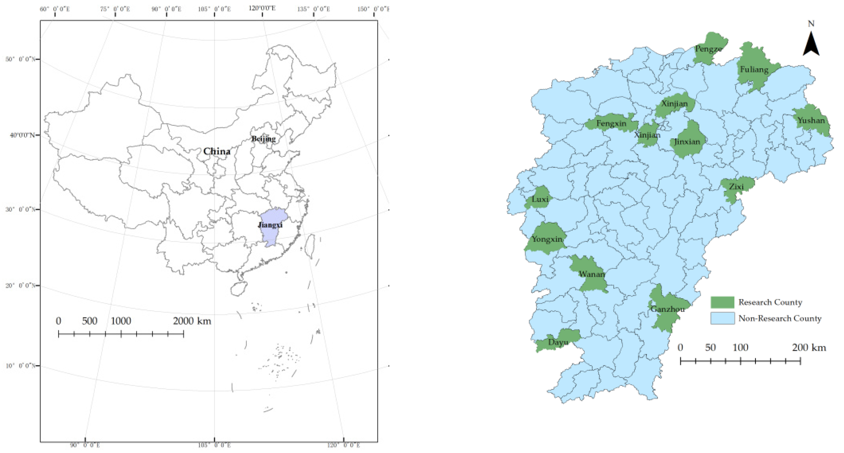
3.2.1. Data Sources

The data in this paper came from the 100 Villages and 1000 Households survey in Jiangxi Province, China. The survey was jointly conducted by Peking University and Jiangxi Agricultural University in December 2018. Jiangxi is a major agricultural province and it is nationally representative of AEE. The sampling group was in accordance with the per capita value of industrial output from Jiangxi Province. We randomly selected twelve counties from the sample county and then, according to the per capita public revenue as the standard, three randomly stratified townships were selected. In accordance with the topography and regional distribution, we next randomly selected three administrative villages. In each village, we randomly selected 10 farmers to conduct household surveys. The sample counties selected by the research group covered the northern, central, and southern regions of Jiangxi Province. A total of 1080 farm households from 108 villages were surveyed in this research. Data on crop growers, including rice and cash crops, were selected and 743 growers were obtained. Invalid questionnaires with missing data and logical errors were deleted and, ultimately, 711 valid surveys were obtained. We used software ArcGIS10.8 to visualize and express the research area (Figure 2).

3.2.2. Variable Selection

The explanatory variable is AEE, which is estimated using the non-desired output super-efficiency SBM model. Land inputs, labor inputs, and capital inputs are selected as input variables, which are the sown area of crops, labor hours of the crop cultivation of farmers, and the costs of agricultural operations (seedlings, pesticides, fertilizers, etc.), respectively (

Table 1. Input–output variables of AEE.

Variable Category	Variable	Variable Definition	Mean	Std Dev.
Input indicators	Land input	Sown area of crops (mu, unit of area equal to one-fifteenth of a hectare)	10.162	29.350
	Labor input	Labor hours of the crop cultivation of farmers (hours)	203.404	392.238
	Capital investment	Costs of agricultural operations (yuan)	5441.639	15,097.510
Desired output	Total output value of agriculture	Output value of grain crops, such as rice, wheat, and cash crops (yuan)	12,973.900	37,697.110
Non-desired output	Agricultural surface pollution	Fertilizer pollution (kg)	398.355	1267.816
		Amount of pesticide contamination (kg)	20.817	88.092

). The total output value of agriculture is taken as the desired output, including the output value of grain crops, such as rice, wheat, and cash crops. The agricultural surface pollution is taken as the non-desired output, including the inefficiency of chemical fertilizers and pesticides. Agricultural surface pollution is characterized by the amount of fertilizer loss and pesticide residue. The amount of fertilizer pollution is determined by multiplying the applied fertilizer application by the fertilizer loss rate (and likewise with pesticide). The pollutant loss rate refers to the existing literature [36,37], with a fertilizer loss rate of 65% and a pesticide pollution rate of 50%.

(1) The core explanatory variable in this paper is agricultural socialized services, i.e., whether farmers use AS, including seeding services, plant protection services, plowing services, rice planting services, and fertilization. (2) The price of socialized services. The price paid by farmers per unit area of socialized services has a key role in the decision to use it; thus, this variable was chosen to be included in the equation. (3) Cost of socialized services. For farmers who use the services, the cost of services and reallocation of resources brought about by the cost of services has an impact on farmers’ AEE.

Referring to Yin et al.’s [38] method of setting instrumental variables, we selected the ratio of service adoption in the same village as an instrumental variable, i.e., the number of farm households in the same village adopting AS other than this one. This has a direct impact on the adoption behavior of this farmer’s participation in AS but does not have a direct effect on the production and management efficiency of the farmer, which is in line with the requirements of instrumental variables.

The control variables included the characteristics of agricultural operations, household characteristics, and head of household characteristics to try to avoid bias in the estimation process. The characteristics of agricultural operations included the agricultural structure, scale of agricultural cultivation, value of agricultural production equipment, and land transfer. Household head characteristics included the age of the head of the household, education level, and whether or not the head of the household received agricultural technology training. Household characteristics included the degree of part-time employment and the number of laborers (

Table 2. Definitions of the main explanatory variables and their descriptive statistical results.

Variable	Variable Definition	Mean	Std. Dev.
Agricultural socialized services	Whether farmers use agricultural socialized services (yes = 1, no = 0)	0.748	0.434
Prices of socialized services	Price of services (yuan/mu)	104.763	50.960
Cost of socialized services	Cost of services (yuan)	821.709	1257.376
Scale of agricultural cultivation	Land cultivation area (mu)	5.921	6.269
Agricultural structure	Percentage of cash crop output	0.156	0.314
Value of agricultural production equipment	Value of agricultural machinery owned by farmers (yuan)	3.158	4.076
Agricultural technology training	Has the farmer received training in agricultural technology? (yes = 1, no = 0)	0.091	0.288
Land transfer	Is there an inflow of land? (yes = 1, no = 0)	3.464	15.004
Extent of part-time work in the household	Proportion of household non-farm labor force (%)	0.373	0.484
Number of laborers	Number of family laborers (persons)	2.848	1.165
Age of head of household	Actual age of head of household (years)	57.461	9.878
Whether the head of household is a village cadre	Whether the head of household is a village secretary, village chief, or member of the village committee (yes = 1, no = 0)	0.210	0.407
Educational level of the head of household	Actual number of years of schooling of the head of household (years)	8.051	6.559

).

4. Empirical Analysis

4.1. Calculation of Green Productivity in Agriculture

We calculated the AEE based on the above non-desired output super-efficiency SBM model. The calculated AEE can be further decomposed into pure technical efficiency and scale efficiency. This result is slightly improved compared with the value of 0.339 of the AEE in Jiangxi Province from 2004 to 2015, as measured by Wang et al. [39]. However, the mean value of the AEE of farmers is still at a lower level. The difference in AEE between farmers is larger, indicating that AEE in Jiangxi Province still has considerable room for improvement so as to continually promote the green transformation of agriculture.

AEE among farmers differed considerably. To better illustrate this paper’s findings, we referred to existing research. The AEE of farmers was classified into a high-efficiency group greater than or equal to 1, a medium-efficiency group greater than 0.8 and less than or equal to 1, and a low-efficiency group of less than 0.8. From the results, it can be seen that the mean values of ecological comprehensive efficiency and pure technical efficiency are low; the proportions of farmers in the high-efficiency group are 4.22% and 5.77% in the comprehensive efficiency and pure technical efficiency group, respectively. The proportions of farmers in the medium-efficiency group are 1.55% and 3.38%, respectively, and the proportions of farmers in the low-efficiency group are 94.2% and 90.9%, respectively (

Table 3. Calculation results of the AEE of farmers.

Groups	Comprehensive Efficiency		Pure Technical Efficiency		Scale Efficiency
	Number	Mean	Number	Mean	Number	Mean
High-efficiency Group	30	1.321	41	1.928	3	1.498
Medium-efficiency group	11	0.847	24	0.927	562	0.929
Low-efficiency group	670	0.312	646	0.342	146	0.591
Total groups	711	0.363	711	0.453	711	0.862

). The results indicate that there is a great potential to expand the number of farmers in the medium-efficiency group to improve AEE.

4.2. Empirical Study of the Effect of Socialized Services on AEE

The ESR model was used to examine the effect of AS on AEE. The results are shown in

Table 4. Endogenous switching model of the effect of AS on AEE.

Variable	Selection Equations (Whether to opt for Socialized Services)		Resulting Equations
			Use Group		Non-Use Group
	Coef.	SE	Coef.	SE	Coef.	SE
Prices of socialized services	−0.0013 *	0.0008
Cost of socialized services			−0.0288 ***	0.010
Scale of agricultural cultivation	0.0010	0.0077	0.0104 ***	0.0026	0.0003	0.003
Agricultural structure	−1.0890 ***	0.1488	0.0422 ***	0.0490	0.3854 ***	0.0649
Value of agricultural production equipment	0.0026	0.0140	0.0015	0.0028	0.0122 **	0.0060
Agricultural technology training	0.2084	0.2029	0.1020	0.0380	−0.1948 **	0.0863
Land transfer	0.0033	0.0047	0.0021	0.0007	−0.0005	0.0021
Extent of part-time work in the household	−0.0796	0.1214	−0.0244	0.0251	0.0217	0.0515
Number of laborers	0.0184	0.0449	0.0107	0.0092	0.0079	0.0191
Age of the head of household	−0.0074	0.0060	−0.0019	0.0013	0.0030	0.0025
Whether the head of household is a village cadre	0.0956	0.1356	0.0737	0.0270	0.0622	0.0586
Educational level of the head of household	0.0003	0.0076	−0.0025	0.0016	0.0020	0.0032
Percentage of adoption of same-village services	0.6234 ***	0.1690
Constant	0.9122 **	0.4259	0.5680 ***	0.1076	−0.4847 ***	0.1710
${\rho }_{Y\epsilon 1}\mathrm{or}{\rho }_{N\epsilon 1}$			−1.4106 ***	0.0316	−0.8871 ***	0.0671
${\chi }^2\left(2\right)$	52.32 ***

Note: *, **, and ***, respectively, indicate significance at the 10%, 5%, and 1% levels.

. The model is divided into two stages. The first stage is the selection equation, which is the probability of farmers choosing AS. Both the agricultural structure and the price of AS inhibit the adoption of services by farmers. The second stage is the outcome equation, which estimates the impact of the farmers’ adoption of socialized services on AEE. For the use group, the agricultural structure and agricultural cultivation scale significantly contribute to AEE while the cost of AS inhibits AEE. For the non-adoption group, the agricultural structure has a contributing effect on AEE.

Our study focused on the impact of AS on AEE. As shown in

Table 5. Measurement of the treatment effect of farmers’ use of AS on AEE in agriculture.

Process	Decision-Making Phase: Use Group	Decision-Making Phase: Non-Use Group	ATT
Coefficient value	0.2796	0.1477	0.1319 ***
Standard error	0.0067	0.0098	0.0160

Note: *** indicate significance at the 1% level.

, the ATT of AEE for the use group is 0.1319. The ATT indicates that for the use group, there is an increase in their AEE after use, confirming H1.

The results in Table 4 and Table 5 show that AS can effectively enhance the AEE of farmers. However, the price of AS discourages farmers from adopting the services. The crowding out of the cost of AS and the reallocation of resources weaken the effect of AS on AEE. Among users, farmers with ample farmland have higher AEE, possibly because larger farmers have more room for negotiation when using the services and the cost of the services has the effect of maximizing the price.

4.3. Heterogeneity Analysis

There may be some differences in the effects of AS on AEE under the constraints of different scales and agricultural structures. We introduce an interaction term between AS and agricultural cultivation scale (Model 2) and an interaction term between AS and agricultural structure (Model 3) to examine the moderating role of the agricultural cultivation scale and the agricultural structure of the impact of AS on AEE.

Table 6. Results of heterogeneity analysis.

Variable	Model 1	Model 2	Model 3
Agricultural socialized services	0.1589 ** (0.0714)	0.1572 ** (0.0711)	0.1552 ** (0.0729)
Scale of agricultural cultivation	0.0035 ** (0.0016)	0.0005 (0.0020)
Agricultural structure	0.0304 (0.0333)		0.0145 (0.0585)
Socialized services × scale of agricultural cultivation		0.0090 *** (0.0034)
Socialized services × agricultural structures			−0.1953 ** (0.0893)
Control variable	yes	yes	yes
Prob > chi2	0.0000	0.000	0.0000

Note: ** and ***, respectively, indicate significance at the 5% and 1% levels, standard errors in parentheses.

shows that the coefficient of AS in Model 2 is significantly positive and the interaction term between AS and agricultural cultivation scale is significantly positive, indicating that the agricultural cultivation scale strengthens the effect of using socialized services on AEE. The interaction term between agricultural structure and AS in Model 3 is significantly negative, indicating that agricultural structure weakens the effect of AS on AEE.

The results show that the impact of AS on AEE differs across different scales and agricultural structures. As the scale of agricultural cultivation increases, the impact of AS on AEE is more pronounced. One possible explanation for this is that the larger the scale of agricultural cultivation, the stronger the scale effect of the AS. The larger the scale, the more farmers may operate roughly due to their own limited agricultural production capacity. By using AS, they can supplement the shortcomings of rural labor shortage and backward production technology. When the proportion of cash crops in the agricultural structure is higher, the impact of AS on AEE is weaker. AS services targeting food production are more common and mature, cash crops are more diverse, and AS targeting cash crops require more refinement and specialization and, therefore, fewer and more expensive service providers. Thus, the impact of AS on AEE is weaker with a higher proportion of cash crops.

4.4. Spatial Spillover Effects of AS on the AEE of Farm Households

4.4.1. Econometric Modeling and the Construction of Spatial Weighting Matrices

Constructing a reasonable spatial weight matrix W to reflect the interconnections among farm households is a prerequisite step for spatial econometric analysis. The production and business activities of farmers are inevitably affected by neighboring farmers. The intensity of this influence depends on the geographic distance of neighboring farmers. The neighboring weight matrix W is set according to the different distances of farmers. Farmers belonging to the same administrative area are set to 1 and otherwise to 0. Considering the progress of the social and economic levels and the increase in transportation convenience, the social interactions between farmers are not necessarily confined to the village administrative area. There are also cross-district operations of agricultural machinery; thus, we set up three neighboring weight matrices to take into consideration the distances of farmers at the village, township, and county levels.

The formulas for the neighborhood spatial weight matrices are expressed as:

$${\mathrm{w}}_{{}_{ij}}^1\{\begin{array}{l}1,\mathrm{Farmer}\mathrm{i}\mathrm{is}\mathrm{in}\mathrm{the}\mathrm{same}\mathrm{administrative}\mathrm{village}\mathrm{as}\mathrm{farmer}\mathrm{j}\\ 0,\mathrm{Farmer}\mathrm{i}\mathrm{is}\mathrm{in}\mathrm{a}\mathrm{different}\mathrm{administrative}\mathrm{village}\mathrm{from}\mathrm{farmer}\mathrm{j}.\end{array}$$

(6a)

$${\mathrm{w}}_{\mathrm{ij}}^2\{\begin{array}{l}1,\mathrm{Farmer}\mathrm{i}\mathrm{is}\mathrm{in}\mathrm{a}\mathrm{same}\mathrm{town}\mathrm{from}\mathrm{farmer}\mathrm{j}\\ 0,\mathrm{Farmer}\mathrm{i}\mathrm{is}\mathrm{in}\mathrm{a}\mathrm{different}\mathrm{town}\mathrm{from}\mathrm{farmer}\mathrm{j}\end{array}$$

(6b)

$${\mathrm{w}}_{\mathrm{ij}}^3\{\begin{array}{l}1,\mathrm{Farmer}\mathrm{i}\mathrm{is}\mathrm{in}\mathrm{the}\mathrm{same}\mathrm{county}\mathrm{as}\mathrm{farmer}\mathrm{j}\\ 0,\mathrm{Farmer}\mathrm{i}\mathrm{is}\mathrm{in}\mathrm{the}\mathrm{different}\mathrm{county}\mathrm{as}\mathrm{farmer}\mathrm{j}\end{array}$$

(6c)

4.4.2. Spatial Spillover Effects

The models under the three weight matrices were regressed separately. The results are shown in

Table 7. Estimated results of the SLX model.

Variable	Matrix W1	Matrix W2	Matrix W3
Agricultural socialized services	0.1540 ** (0.0712)	0.1532 ** (0.0711)	0.1752 ** (0.0709)
W Agricultural socialized services	0.0943 ** (0.0405)	0.1468 *** (0.0524)	0.2859 *** (0.0794)
Costs of agricultural socialized services	−0.0222 ** (0.0107)	0.0344 (0.0332)	0.0492 (0.0334)
Scale of agricultural cultivation	0.0031 * (0.0016)	−0.0005 (0.0012)	−0.0003 (0.0012)
Agricultural structure	0.0298 (0.0332)	−0.0011 (0.0015)	−0.0010 (0.0015)
Value of agricultural production equipment	0.0059 ** (0.0026)	0.0858 *** (0.0250)	0.0848 *** (0.0249)
Agricultural technology training	0.0361 (0.0357)	0.0425 (0.0355)	0.0521 (0.0355)
Land transfer	0.0020 *** (0.0007)	0.0055 ** (0.0026)	0.0058 ** (0.0026)
Extent of part-time work in the household	−0.0160 (0.0231)	0.0018 *** (0.0007)	0.0017 ** (0.0007)
Number of laborers	0.0105 (0.0085)	0.0032 * (0.0016)	0.0029 * (0.0016)
Age of head of household	−0.0005 (0.0012)	−0.0175 (0.0230)	−0.0130 (0.0230)
Whether the head of household is a village cadre	0.0862 *** (0.0251)	0.0109 (0.0085)	0.0113 (0.0084)
Educational level of the head of household	−0.0013 (0.0015)	−0.0224 ** (0.0106)	−0.0246 ** (0.0106)
Constant	0.2279 *** (0.0804)	0.1885 ** (0.0837)	0.0604 (0.0978)

Note: *, **, and ***, respectively, indicate significance at the 10%, 5%, and 1% levels.

. The SLX model is not needed to measure the direct and indirect effects further and the spatial lag term of the socialized service variable reflects the spatial spillover effect. When the neighboring distance is at the village level, both the direct and indirect effects of socialized services are positive and significant, indicating that the use of AS by farmers promotes their own AEE and produces a positive spillover effect on neighboring farmers. When the neighboring relationship is at the township and county levels, the socialized services both promote the AEE of the farmers. For different distance thresholds, the extent of the spillover effect of socialized services on AEE tends to increase gradually with distance. Possible explanations for this are that there is mutual imitation among farmers. The gradual spread of agricultural technology and the cross-district operation of agricultural machinery help to increase the farms’ AEE.

5. Discussion

5.1. The Impact of Service Scale or Land Scale on AEE

A large country and small farmers are the characteristics of Chinese agriculture. However, small farming operations have many disadvantages, especially in terms of the scale of economies. The scale of agricultural operations can improve the efficiency of the scale of operations, reduce the cost of agricultural production, and improve the efficiency of production and centralization, which is the global trend in agriculture. In contrast to the United States, where large-scale farms dominate with characteristics such as modernization, formalization, and specialization, Asia has a significant presence of small-scale agricultural operations. For example, more than 90% of agricultural operating areas are less than 1 hectare in China, followed by India at around 65% and other Asian countries averaging at 60% [40]. In Africa, the proportion of agricultural operations of less than 1 hectare is about 55%. The advantage of smallholder farmers is agricultural intensification; however, long-term reliance on this high-input model of agricultural production has resulted in environmental problems, such as declining soil fertility, agricultural surface pollution, and carbon emissions [41]. These problems may be even more severe in developing countries. In China, the use of chemical fertilizers has significantly increased from 8.84 million tons in 1978 to 51.913 million tons in 2020, leading to severe soil and water pollution.

Many countries have taken various measures to address the plight of smallholder farmers. The Japanese government has strongly supported the development of agricultural associations [42] while South Korea has initiated a reform of its land system based on private land ownership [43]. In addition, India has launched a green revolution with government support [44]. The Chinese government has also made many efforts, such as promoting the transfer of land to facilitate large-scale agricultural operations. However, after more than three decades of policy promotion, the pattern of decentralized land management in China has not changed. With the evolution of marketization and specialized division of labor, farmers can replace the scale operation of farmland with the scale operation of services in a roundabout way by purchasing productive services. We confirm that AS promote AEE by increasing production efficiency and reducing the use of agrochemicals in this paper, as demonstrated by Zhang et al. [13]. China’s experience provides a reference for developing countries in Asia and in Africa, where small-scale farmers predominate.

5.2. The Impact of AS on AEE under Different Cropping Structures

This paper explores the impact of AS on AEE based on farm household research data in Jiangxi Province. The findings suggest that when the proportion of cash crops in the agricultural structure is higher, the impact of AS on AEE is weaker. Jiangxi Province is recognized as one of China’s 13 main grain-producing regions. Data from China’s Rural Statistical Yearbook indicate that in 2018, the proportion of grain cultivation in Jiangxi Province was 66.98%, which is similar to the average proportion of grain cultivation in China’s 31 provinces (65.41%). China attaches great importance to food security and the central government’s Document No. 1 emphasizes the development of AS to achieve cost reduction and efficiency increase in agricultural production and to guarantee the country’s food security. As a result, the development of AS around food production in a number of segments, such as plowing, fertilizing, dosing, harvesting, etc., is more mature, providing diversified choices for small farmers. AS organizations can improve production efficiency and reduce chemical inputs by uniformly purchasing agricultural production materials and implementing large-scale mechanized operations. Because of the characteristics of Jiangxi Province’s own agricultural structure, the AS for food production are more common and mature while the types of cash crops are more diverse. The AS for cash crops require more refinement and specialization and cash crops account for a smaller share of the cultivation. Luo et al. [24] point out that if the scale of services for the farmers is limited, they cannot induce the supply of AS. Therefore, service providers are also fewer and more expensive, which leads to biasing the agricultural structure of farmers towards cash crops and inhibiting the impact of AS on AEE.

However, due to China’s vast area, the agricultural structure varies significantly across different regions. This research paper specifically focuses on the main grain-producing area in Jiangxi Province, where farmers are more engaged in grain production. This paper does not take into account the provinces that are dominated by cash crops, such as the Xinjiang Uygur Autonomous Region. Cash crops account for 63.43% of the total cultivated area in Xinjiang, which is a major cotton production area, with cotton alone occupying 41.05% of the area. Thus, the proportion of the area planted with cash crops is much higher than that of the grain production area. Consequently, the findings of this paper may not be applicable to provinces that are primarily represented by cash crops.

5.3. Limitations and Future Research

Although this paper has certain theoretical and practical significance, it still has certain limitations. First of all, the research objects selected in this paper are all from Jiangxi Province, which is a large agricultural province, and there is a lack of surveys in other provinces, which cannot represent all agricultural provinces in the country. In the future, the research sample can be expanded to study the situation in different regions. Secondly, the data in this paper come from field surveys in a single year and lack the observation of time series. In future research, try to strengthen the tracking survey of the sample farmers to analyze the long-term impact of AS on AEE. The independent variable in this paper is whether farmers adopt AS but it is not broken down into specific segments; future research could consider the impact of farmers’ AS on AEE in different production segments of agricultural production, such as pre-production, mid-production, and post-production. The scope should be expanded in the future to explore the long-term impact of improving AEE.

6. Conclusions and Implications

6.1. Conclusions

In this study, we examine the impact of AS on AEE from the perspective of promoting sustainable agricultural development and analyze its spillover effects. The results of this study are as follows. (1) The mean value of AEE is 0.363, which is at a low level with considerable room for improvement. (2) AS significantly increase AEE, specifically, the AEE of farmers who adopted the services increased by 13.19% relative to those who did not. In addition, the results of heterogeneity analysis showed that the larger the scale of agricultural cultivation, the stronger the impact of AS on AEE. We also found that a larger share of cash crops inhibits the impact of socialized services on AEE. (3) Further, by constructing a spatial econometric model, we tested the existence of the spatial spillover effects of AS on AEE. We demonstrated the existence of mutual learning and imitation among farmers and, by constructing different distance thresholds, we found that the degree of impact of AS on AEE tends to increase with distance.

6.2. Managerial Implications

Based on the results of this study, we make the following recommendations. Our findings have several policy implications. First, the price of AS discourages farmers from using them and, hence, potential improvements in AEE. Therefore, there is an urgent need to reduce the price of AS; the government should strengthen public welfare AS and provide appropriate subsidies to commercial AS organizations so as to reduce the cost of AS and improve the theoretical and practical skills of practitioners. The government should continue to improve the AS network, forming a three-tier service system of “county, township, and village” and expanding the audience for AS. Secondly, the current service organizations have weak service capacity. Single service projects and other issues need to be improved for food crops, without ignoring the demand for social services for cash crops. Cash crops are more valuable and they can enhance the income of farmers; however, it is difficult to plant cash crops and professional knowledge is needed. There is a need for social service organizations to provide more detailed and professional services. Finally, the demonstration role of farmers should be given full play to promote the exchange and diffusion of production information and technology among farmers and to strengthen the interoperability of farmers at all levels. This will enhance the overall green production awareness of farmers, thereby reducing the excessive application of agricultural chemicals, reducing agricultural pollution, and promoting the green transformation of agriculture.

References

1. Jin, G.; Li, Z.; Deng, X.; Yang, J.; Chen, D.; Li, W. An Analysis of Spatiotemporal Patterns in Chinese Agricultural Productivity between 2004 and 2014. Ecol. Indic. 2019, 105, 591–600. [Google Scholar] [CrossRef]
2. Alwyn, Y. The Tyranny of Numbers: Confronting the Statistical Realities of the East Asian Growth Experience. Q. J. Econ. 1995, 110, 641–680. [Google Scholar]
3. Solow, R.M. Technical Change and the Aggregate Production Function. Rev. Econ. Stat. 1957, 39, 312. [Google Scholar] [CrossRef]
4. Repetto, R.; Rothman, D.; Faeth, P.; Austin, D. Has Environmental Protection Really Reduced Productivity Growth? Challenge 1997, 40, 46–57. [Google Scholar] [CrossRef]
5. Nanere, M.; Fraser, I.; Quazi, A.; D’Souza, C. Environmentally Adjusted Productivity Measurement: An Australian Case Study. J. Environ. Manag. 2007, 85, 350–362. [Google Scholar] [CrossRef] [PubMed]
6. Cai, J.; Xu, X.; Yu, T. Performance Evaluation of Resource Utilization with Environmental Externality: Evidence from Chinese Agriculture. J. Clean. Prod. 2023, 397, 136561. [Google Scholar] [CrossRef]
7. Rausser, G.; Zilberman, D. Government Agricultural Policy, United States. In Encyclopedia of Agriculture and Food Systems; Elsevier: Amsterdam, The Netherlands, 2014; pp. 518–528. [Google Scholar]
8. Jiuhardi, J.; Hasid, Z.; Darma, S.; Darma, D.C. Sustaining Agricultural Growth: Traps of Socio–Demographics in Emerging Markets. Oppor Chall. Sustain. 2022, 1, 13–28. [Google Scholar] [CrossRef]
9. Liu, Y.; Zou, L.; Wang, Y. Spatial-Temporal Characteristics and Influencing Factors of Agricultural Eco-Efficiency in China in Recent 40 Years. Land Use Policy 2020, 97, 104794. [Google Scholar] [CrossRef]
10. Dhananjayan, P.; Koirala, P.; Sharma, D. Advancing Sustainable Development in the Hindu-Kush-Himalaya Region Through Certification Strategies. Oppor Chall. Sustain. 2023, 2, 93–103. [Google Scholar] [CrossRef]
11. Coluccia, B.; Valente, D.; Fusco, G.; De Leo, F.; Porrini, D. Assessing agricultural eco-efficiency in Italian Regions. Ecol. Indic. 2020, 116, 106483. [Google Scholar] [CrossRef]
12. Nsiah, C.; Fayissa, B. Trends in Agricultural Production Efficiency and their Implications for Food Security in Sub-Saharan African Countries. Afr. Dev. Rev. 2019, 31, 28–42. [Google Scholar] [CrossRef]
13. Zhang, P.; Lu, H.; Geng, X.; Chen, Y. How Do Outsourcing Services Affect Agricultural Eco-Efficiency? Perspectives from Farmland Scale and Technology Substitution. J. Environ. Plan. Manag. 2023, 45, 1–25. [Google Scholar] [CrossRef]
14. Li, Z.; Ye, W.; Jiang, H.; Song, H.; Zheng, C. Impact of the Eco-Efficiency of Food Production on the Water–Land–Food System Coordination in China: A Discussion of the Moderation Effect of Environmental Regulation. Sci. Total Environ. 2023, 857, 159641. [Google Scholar] [CrossRef] [PubMed]
15. Zeng, L.; Li, X.; Ruiz-Menjivar, J. The Effect of Crop Diversity on Agricultural Eco-Efficiency in China: A Blessing or a Curse? J. Clean. Prod. 2020, 276, 124243. [Google Scholar] [CrossRef]
16. Li, L.; Han, J.; Zhu, Y. Does Farmland Inflow Improve the Green Total Factor Productivity of Farmers in China? An Empirical Analysis Based on a Propensity Score Matching Method. Heliyon 2023, 9, e13750. [Google Scholar] [CrossRef] [PubMed]
17. Zou, X.; Xie, M.; Li, Z.; Duan, K. Spatial Spillover Effect of Rural Labor Transfer on the Eco-Efficiency of Cultivated Land Use: Evidence from China. Int. J. Environ. Res. Public Health 2022, 19, 9660. [Google Scholar] [CrossRef] [PubMed]
18. Zong, Y.; Ma, L.; Shi, Z.; Gong, M. Agricultural Eco-Efficiency Response and Its Influencing Factors from the Perspective of Rural Population Outflowing: A Case Study in Qinan County, China. Int. J. Environ. Res. Public Health 2023, 20, 1016. [Google Scholar] [CrossRef]
19. Tang, L.; Liu, Q.; Yang, W.; Wang, J. Do Agricultural Services Contribute to Cost Saving? Evidence from Chinese Rice Farmers. CAER 2018, 10, 323–337. [Google Scholar] [CrossRef]
20. Deng, X.; Xu, D.; Zeng, M.; Qi, Y. Does Outsourcing Affect Agricultural Productivity of Farmer Households? Evidence from China. CAER 2020, 12, 673–688. [Google Scholar] [CrossRef]
21. Zang, L.; Wang, Y.; Ke, J.; Su, Y. What Drives Smallholders to Utilize Socialized Agricultural Services for Farmland Scale Management? Insights from the Perspective of Collective Action. Land 2022, 11, 930. [Google Scholar] [CrossRef]
22. Zhang, C.; Hu, R.; Shi, G.; Jin, Y.; Robson, M.G.; Huang, X. Overuse or Underuse? An Observation of Pesticide Use in China. Sci. Total Environ. 2015, 538, 1–6. [Google Scholar] [CrossRef] [PubMed]
23. Chen, Y.; Lu, H.; Luo, J. How Does Agricultural Production Outsourcing Services Affect Chemical Fertilizer Use under Topographic Constraints: A Farm-Level Analysis of China. Environ. Sci. Pollut. Res. 2023, 30, 100861–100872. [Google Scholar] [CrossRef] [PubMed]
24. Luo, B. 40-Year Reform of Farmland Institution in China: Target, Effort and the Future. CAER 2018, 10, 16–35. [Google Scholar] [CrossRef]
25. Qing, C.; Zhou, W.; Song, J.; Deng, X.; Xu, D. Impact of Outsourced Machinery Services on Farmers’ Green Production Behavior: Evidence from Chinese Rice Farmers. J. Environ. Manag. 2023, 327, 116843. [Google Scholar] [CrossRef] [PubMed]
26. Zhou, H.; Yan, J.; Lei, K.; Wu, Y.; Sun, L. Labor Migration and the Decoupling of the Crop-Livestock System in a Rural Mountainous Area: Evidence from Chongqing, China. Land Use Policy 2020, 99, 105088. [Google Scholar] [CrossRef]
27. Pan, D.; He, M.; Kong, F. Risk Attitude, Risk Perception, and Farmers’ Pesticide Application Behavior in China: A Moderation and Mediation Model. J. Clean. Prod. 2020, 276, 124241. [Google Scholar] [CrossRef]
28. Wu, Y.; Xi, X.; Tang, X.; Luo, D.; Gu, B.; Lam, S.K.; Vitousek, P.M.; Chen, D. Policy distortions, farm size, and the overuse of agricultural chemicals in China. Proc. Natl. Acad. Sci. USA 2018, 115, 7010–7015. [Google Scholar] [CrossRef]
29. Li, Y.; Huan, M.; Jiao, X.; Chi, L.; Ma, J. The Impact of Labor Migration on Chemical Fertilizer Use of Wheat Smallholders in China- Mediation Analysis of Socialized Service. J. Clean. Prod. 2023, 394, 136366. [Google Scholar] [CrossRef]
30. Tone, K. A slacks-based measure of efficiency in data envelopment analysis. Eur. J. Oper. Res. 2001, 130, 498–509. [Google Scholar] [CrossRef]
31. Yang, H.; Wang, X.; Bin, P. Agriculture Carbon-Emission Reduction and Changing Factors behind Agricultural Eco-Efficiency Growth in China. J. Clean. Prod. 2022, 334, 130193. [Google Scholar] [CrossRef]
32. Ma, W.; Renwick, A.; Nie, P.; Tang, J.; Cai, R. Off-Farm Work, Smartphone Use and Household Income: Evidence from Rural China. China Econ. Rev. 2018, 52, 80–94. [Google Scholar] [CrossRef]
33. Tesfay, M.G. Does Fertilizer Adoption Enhance Smallholders’ Commercialization? An Endogenous Switching Regression Model from Northern Ethiopia. Agric. Food Secur. 2020, 9, 3. [Google Scholar] [CrossRef]
34. Ying, R.; Xu, B. Analysis of the demonstration effect of farmers’ adoption of agricultural socialized services—An example of pest control. China Rural. Econ. 2014, 8, 30–41. [Google Scholar]
35. Niu, Z.; Chen, C.; Gao, Y.; Wang, Y.; Chen, Y.; Zhao, K. Peer effects, attention allocation and farmers’ adoption of cleaner production technology: Taking green control techniques as an example. J. Clean. Prod. 2022, 339, 130700. [Google Scholar] [CrossRef]
36. Lai, S.Y.; Du, P.F.; Chen, J.N. A non-point source pollution investigation and assessment method based on unit analysis. J. Tsinghua Univ. (Nat. Sci. Ed.) 2004, 9, 1184–1187. [Google Scholar]
37. Wu, S.Q.; Wang, Y.P.; He, L.M.; Lu, G. Evaluation of agricultural eco-efficiency based on AHP and DEA modeling—Taking Wuxi City as an example. Yangtze River Basin Resour. Environ. 2012, 21, 714–719. [Google Scholar]
38. Yin, C.C.; Gan, L. Cigarettes, Wine and Income. Econ. Res. 2010, 45, 90–100. [Google Scholar]
39. Wang, B.-Y.; Zhang, W.-G. Interprovincial differences and influencing factors of agroecological efficiency in China—A panel data analysis based on 31 provinces from 1996 to 2015. China Rural. Econ. 2018, 1, 46–62. [Google Scholar]
40. FAO. Investing in Smallholder Agriculture for Food Security. A Report by the High Level Panel of Exports on Food Security and Nutrition. Available online: http://www.fao.org/docrep/018/i2953e/i2953e.pdf (accessed on 12 May 2022).
41. Bryan, B.A.; Gao, L.; Ye, Y.; Sun, X.; Connor, J.D.; Crossman, N.D.; Stafford-Smith, M.; Wu, J.; He, C.; Yu, D.; et al. China’s response to a national land-system sustainability emergency. Nature 2018, 559, 193–204. [Google Scholar] [CrossRef]
42. Tanimoto, M. Peasant society in Japan’s economic development: With special focus on rural labour and finance markets. Int. J. Asian Stud. 2018, 15, 229–253. [Google Scholar] [CrossRef]
43. Lee, J.; Oh, Y.-G.; Yoo, S.-H.; Suh, K. Vulnerability assessment of rural aging community for abandoned farmlands in South Korea. Land Use Policy 2021, 108, 105544. [Google Scholar] [CrossRef]
44. Sannigrahi, S.; Pilla, F.; Zhang, Q.; Chakraborti, S.; Wang, Y.; Basu, B.; Basu, A.S.; Joshi, P.K.; Keesstra, S.; Roy, P.S. Examining the effects of green revolution led agricultural expansion on net ecosystem service values in India using multiple valuation approaches. J. Environ. Manag. 2021, 277, 111381. [Google Scholar] [CrossRef] [PubMed]
Figure 1. Analytical framework.
Sustainability 16 00360 g001
Figure 2. Research area in Jiangxi Province. (Source of map: Revision No. GS (2020) 4619, map without modifications).
Sustainability 16 00360 g002