2. Mathematical Formulation of DMFCs
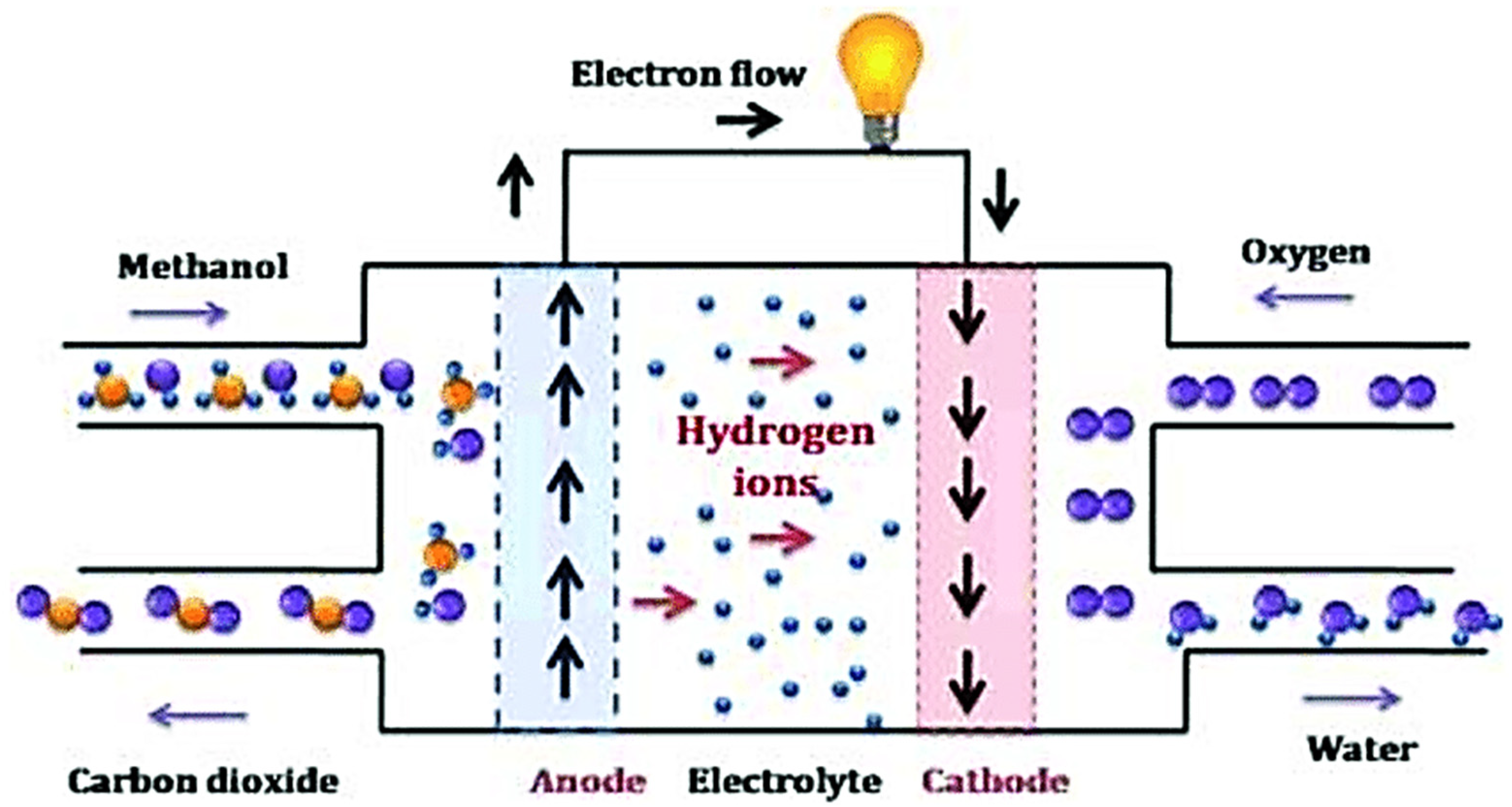
A fuel cell is a device that continuously converts chemical energy into electrical energy and heat. It does not store energy like a battery but instead operates continuously by supplying fuel and oxidants. Unlike engines, fuel cells do not emit greenhouse gases as a result of their output. Therefore, they are considered an environmentally friendly alternative. A schematic of the DMFC stack is presented in
Figure 1, and this study focuses on mathematically modelling the stack. A metaheuristic algorithm called ELSHADE is used to extract unknown parameters in the model. As shown in Equation (1), DMFC cell voltage is expressed as:
The voltage within the cell is shown by , the concentration of the voltage is represented by , the activation voltage is represented by , the reversible voltage is represented by , and the ohmic voltage is represented by .
The electrochemical equation for a direct methanol fuel cell (DMFC) can be represented by the following Equations (2)–(4):
These equations represent the chemical reactions that occur at the anode and cathode of a DMFC. At the anode, methanol and water are oxidised to form carbon dioxide, protons (H+), and electrons (e−). At the cathode, oxygen is reduced to form water. The overall reaction combines the anode and cathode reactions to show that the oxidation of methanol with oxygen produces carbon dioxide, water, and energy in the form of electricity.
2.1. Activation Loss Voltage Expression
The activation voltage is determined by Equation (5), which is the required overvoltage to activate electrodes. The Butler–Volmer equation is employed to calculate the current density,
.
The exchange current density is denoted as
, and the value of α is between 0 and 1. Analytical solutions cannot be found for Equation (5) regarding activation voltage. To address this, the voltage
in the first exponential of the equation is substituted with
,
,
, and
, leading to the following Equation (6):
Equation (7) can be used to represent the expression for the updated activation voltage:
2.2. Ohmic Loss Voltage Expression
The voltage loss attributed to resistance encountered by ions, electrons, and other substances during transport across a membrane is known as “ohmic loss voltage”. Equation (8) below depicts the ohmic voltage [
6]:
The current density and internal resistance r are the variables used to express the ohmic voltage in Equation (8).
2.3. Concentration Loss Voltage Expression
The voltage drop caused by mass transfer is referred to as concentration over potential. Using Fick’s law, the over potential due to concentration can be represented by Equation (9):
Equation (10) provides a brief representation of
, which is used in Equation (9).
The parameter β, an empirical coefficient, and , the limiting current density, are denoted in Equation (10).
2.4. Reversible Loss Voltage Expression
Equation (11) depicts the reversible voltage that arises from the energetic activity involved in the formation and breaking of bonds at the electrode level, which is represented by the Nernst equation [
12]:
The equation for the reaction between methanol and oxygen can be represented by the potential
. The partial pressure of methanol present at the anode is denoted by
. The partial pressure of water at the cathode is represented by
, which equals 1 when liquid water is produced. The partial pressure of oxygen at the cathode is denoted by
. The partial pressure of carbon dioxide is represented by
. The universal gas constant is R (8.314 J/molK), Faraday’s constant is denoted by F (94,485 c/mol), and the number of electrons is represented by n. It is generally not possible to directly measure the pressures of CO
2 and H
2O experimentally. As a result, the term
is assigned a value of C
1, which must be determined empirically. With this modification, the reversible voltage equation can be expressed as shown in Equation (12):
The variable “t” represents the temperature of the cell in Kelvin (K).
2.5. Fuel Cell Voltage Expression
Building on earlier theoretical work, the voltage of the fuel cell (V
cell) can be expressed using Equation (13) below:
With
Equations (13a)–(13e) provide a set of expressions for the seven unknown parameters y in the form y = [,,,,,, req].
2.6. Problem Formulation
In this study, the ELSHADE algorithm is introduced as an enhanced approach to parameter estimation for DMFCs. The algorithm uses optimisation techniques to predict the output voltage for a given current density input. The predicted output voltage is evaluated against the experimental values using SSE (sum of squared errors) as the metric. The objective function for SSE is given by Equation (14):
Equations (15)–(21) present the constraints that apply to the DMFC.
The experimental output voltage is denoted by while represents the predicted output voltage obtained using different optimisation algorithms. With N representing the number of data points, the primary aim of this study is to minimise the SSE value to achieve improved performance, accuracy, and precision when estimating the DMFC parameters.
3. Materials and Methods
The DE approach was first proposed by Storn and Price [
13]. SHADE secured third place in the IEEE CEC2013 competition, while LSHADE emerged as the winner in the CEC2014 competition [
14]. This approach has been highly effective in tackling real-world optimisation problems [
15]. In the basic DE algorithm, the mutation factor (G), crossover rate (DS), and population size (Q) are critical control factors that must be adjusted [
16]. The population size Q consists of individual vectors (OQ), each of which has a decision variable (E). Therefore, j = 1, 2, ……, O
Q and k = 1, 2, ……, E. The maximum number of generations (H
Max) is used as a stopping criterion. Similar to other stochastic population-based search techniques, LSHADE utilises mutation, external archive, parameter adaption, crossover, and selection processes to determine optimal values for the optimisation problem. The LSHADE method can be divided into the following steps:
The first step, initialisation, involves generating an initial population by selecting random values for the decision variables within their feasible boundaries. Equation (22) represents the initialisation of the k-th decision variable’s j-th component [
17]:
A value of is randomly selected from the range [0, 1], where “0” represents the population’s initial state. The next step involves mutation, which creates a random vector for each generation.
In the second step of the process, referred to as mutation, a mutant vector, denoted as
, is generated from each generation of the population using the “current-to-p-best/1” approach [
14]. This mutant vector can be expressed mathematically as shown in Equation (23).
From the OQ, two distinct vectors, namely and , are randomly selected. The refers to the highest-ranking vector from the set of Np*l(l € [0, 1]), where “l” denotes a control parameter that is expected to be small to promote more greedy behaviour. Additionally, represents the mutation scale parameters, which may be varied between generations.
The third step of LSHADE involves the use of an external archive to increase the diversity of the parent vectors, . When utilising the archive, is selected from both the population and the archive Q u B. It is worth noting that Q and B are intended to be of the same size. If the size of the archive exceeds the limit of |B|, then certain items are removed to make room for new entries.
In order to create the offspring vector
, the adaptation of the mutation scale
and crossover rate
parameters is linked to the individual vector
. The adaptation of these two parameters can be achieved through the use of Equations (24) and (25). This constitutes Step 4 of the process.
The values
and
are obtained from the Cauchy and normal distributions, respectively. It is important to note that the
and
values must lie within the range of [0, 1]. In cases where
exceeds 1, it will be truncated, while if it is less than 0, Equation (14) will be iterated until a valid value is obtained. At the beginning of the analysis, N
G and N
DQ are both initialised to 0.5, as described in reference [
15].
Assuming the offspring vector successfully competes with the parent vector at generation H, the current
and
values are considered to be effective and are consequently saved in T
G and T
DQ, respectively. Furthermore, at the conclusion of the generation, the contents of N
G and N
DQ memories are modified utilising the weighted Lehmer mean and weighted arithmetic mean, respectively, as exhibited in Equations (26) and (27) of reference [
15].
The memory location to be updated is determined based on the index “l” which has a memory capacity of (I) where (I ≥ l ≥ 1). Whenever a new element is loaded into memory, the value of “l” is first set to 1 and then incremented. If the value of “l” exceeds the value of I, it is reset to 1. In case the individuals in generation H fail to produce an offspring vector, the memory update process will not take place.
In Step 5, the offspring vector
is created by combining the components of the mutant vector
with the target (parent) vector
using a binomial strategy. This process is represented in Equation (28).
The variable is a random number chosen from the range of [1, E], and represents a value within the range of [0, 1].
In Step 6, a selection process takes place in which the parent and offspring vectors are compared, and the best fitting vector is selected for the subsequent generation. This process is represented by Equation (29).
Step 7 involves the implementation of linear population size reduction in LSHADE, which improves its performance. In this process, the population size is dynamically decreased for every generation using Equation (30) [
14].
The population’s minimum number, denoted by , is assumed to be 4, while represents the initial size of the population. OGF stands for the number of fitness function evaluations, and refers to the maximum number of fitness function evaluations allowed for the population.
3.1. Improved Newton–Raphson Method
Traditional methods such as the NR and Lambert W function techniques are capable of handling nonlinear equations. However, these methods often converge quickly but not globally, leading to unfavourable outcomes. Moreover, their performance in classical form may deviate from the true and accurate root values. Therefore, it is essential to identify global solutions in a concise manner and within a few iterations. To address these concerns, the INR approach is proposed, which effectively improves the efficiency of identifying good initial condition values.
3.2. The Proposed Enhanced Algorithm
To enhance the convergence capabilities of the LSHADE algorithm and increase population diversity, it is split into two halves. The first half uses the “current-to-pbest/1” technique, as shown in Equation (13). In contrast, the second half utilises the guided-chaotic approach, represented by Equation (31) [
18].
Equation (32) provides the expression for the chaotic perturbation, denoted as P.
where
Chaos possesses an advantage due to the presence of pseudo-random patterns in the cycles [
19]. This chaotic distribution is employed to explore new search regions, resulting in a shift in the direction of the search from local to global [
20].


 ,
, 


