Leakage Diffusion Modeling of Key Nodes of Gas Pipeline Network Based on Leakage Concentration

Abstract

In order to achieve the prediction and early warning of city gas pipe network leakage accidents, as well as to provide rapid and precise support for emergency response to such accidents, this study focuses on a Gaussian diffusion model applied to a large urban gas pipeline network. Specifically, it investigates the gas gate wells, which are key nodes in the pipeline network, to develop a leakage model. The objective is to analyze the variation in internal gas concentration in the gate wells and determine the range of danger posed by external gas diffusion from the gate wells. In addition, Fluent simulation is utilized to compare the accuracy of the model’s calculations. The findings of this study indicate that the gas concentration inside the gate well, as predicted by the model fitting results and Fluent simulation, exhibit a high level of agreement, with coefficient of determination (R²) values exceeding 0.99. Moreover, when predicting the hazardous distance of gas leakage outside the gate well, the model’s results show an average relative error of 0.15 compared to the Fluent simulation results. This demonstrates that the model is highly accurate and meets the practical application requirements.

1. Introduction

As the most practical and economical means of transporting natural gas in urban areas, pipelines are extensively utilized on a global scale and significantly contribute to people’s daily lives and the national economy. Traditionally, natural gas pipelines are buried directly beneath roads. However, with the improvement of the economy and the acceleration of urbanization, there is an increasing strain on the supply of urban infrastructure, necessitating the continual expansion of underground pipelines [1,2]. However, natural gas pipelines often experience leaks due to corrosion, natural disasters, and third-party damage. These leaks not only result in resource waste and environmental pollution but also pose significant risks to infrastructure and public safety, as natural gas is highly flammable and explosive. Furthermore, these incidents have been known to cause numerous fatalities and injuries [3,4]. These examples further illustrate the devastating consequences of natural gas pipeline leaks. The explosion in Manhattan, New York, in 2014 resulted in injuries and a significant loss of lives. Similarly, the gas explosion in Hubei Province, China, in 2021 caused numerous fatalities, injuries, and substantial economic damage. These incidents highlight the urgency of addressing the issue of natural gas pipeline leaks to prevent such tragedies in the future [5]. Gas gates serve as essential means for regulating and controlling key facilities within gas networks. These gates are strategically placed at various nodes throughout the gas pipeline network. In line with the gas industry’s status, certain modern gas gates have been equipped with a remote cut-off function, enabling remote shut-off in the case of gas leakage. The equipment in these gas gates is equipped with remote monitoring and control systems that can establish a connection with a central control center through remote communication technology. When a gas leakage event occurs, the central control center promptly receives the relevant alarm information and takes immediate action based on the situation. Through the remote control system, operators can remotely shut off the gas supply to the airlock wells, effectively controlling the leakage situation. This significantly improves the emergency response efficiency of gas companies, reducing the likelihood of gas accidents. However, it is important to note that gas valve wells are a major source of leakage in urban gas networks. Based on past statistics and related research results, many areas experience frequent leakage issues in gas valve wells due to aging pipes, sealing failures, or operational errors. Gas valve well leakage can lead to gas leaks, which in turn may result in explosions, fires, and other safety accidents. These accidents not only pose a threat to human lives but also have adverse effects on the local economy. Gas leaks often cause shutdowns, production stoppages, and emergency repair costs, placing significant strain on the economy. Although some leaks have been promptly addressed, potential risks associated with gas valve shaft leaks still remain. Problems such as aging equipment, inadequate maintenance, and mismanagement of gas valve shafts persist, increasing the likelihood of serious leaks in the future. Therefore, it is crucial not to underestimate the potential risks associated with these issues.

Scholars at home and abroad have primarily conducted research on the diffusion law of gas leakage through three main approaches: experiments, numerical simulations, and theoretical analysis. Sun et al. [6] conducted a series of experiments based on the German Water and Gas Association’s research, analyzing the factors that influence natural gas diffusion underground. These factors include temperature, humidity, road surface covering (asphalt or cement), and the presence of cracks or inspection wells on the road surface. The study emphasized the significance of accurately capturing crucial information such as the amount of gas leakage, leakage rate, diffusion range, and concentration distribution for effective on-site rescue operations. Moghadam et al. [7] performed a study focused on the computational fluid dynamics (CFDs) analysis and prediction of gas leakage and dispersion in underground damaged natural gas pipelines. The research aimed to understand the extent of gas leakage and dispersion in such scenarios using CFDs simulations. Liu et al. [8] performed numerical simulations to analyze the leakage and diffusion characteristics of natural gas in an integrated pipeline corridor under different operating conditions. The study investigated variations in factors such as pressure, leakage diameter, ventilation conditions, and leakage locations. The research examined the effects of single-factor and multifactor variations on the gas leakage and diffusion behavior in the integrated pipeline corridor. Li et al. [9] conducted numerical simulations to investigate the changes in the soil temperature field near a leaking port of a buried gas pipeline. The study aimed to provide a reference for the application of fiber-optic temperature detection technology in detecting leaks in buried gas pipelines. Yan et al. [10] utilized Fluent software (Ansys Fluent 15.0; Ansys Fluent 2021R1) to conduct a non-stationary numerical simulation study on the diffusion process of gas leakage from buried gas pipelines in soil. The study aimed to analyze the effects of various factors, such as changes in pipeline operating pressure, leakage aperture, and soil porosity on the diffusion characteristics of gas in soil. Wang et al. [11] conducted a study on the mechanism of gas leakage diffusion from small holes under natural and mechanical ventilation. They employed Fluent software to simulate and analyze the various factors that influence gas leakage diffusion. Peng et al. [12] conducted a non-stationary numerical simulation study on the diffusion process of leaking gas from buried gas pipelines in soil. They analyzed the effects of various factors such as changes in pipeline operating pressure, leakage aperture, soil porosity, and others on the diffusion characteristics of gas in soil. Zhang et al. [13] developed a simulation model of a gas pipeline within an integrated pipeline corridor using Computational Fluid Dynamics (CFDs) theory. They conducted simulations to study gas leakage and diffusion scenarios under different ventilation speeds and vent sizes. Parvini et al. [14] performed a risk assessment to evaluate the potential consequences of gas leakage from buried pipelines. They assessed a variety of hazards associated with leakage from open-space gas pipelines. Liu et al. [15] conducted a study that explored the diffusion behavior of gas leakage from buried pipelines. They specifically investigated the impact of various building arrangements and ambient wind fields on the dispersion of leaked natural gas. The researchers derived the concentration distribution of the gas and identified the range of hazardous areas under different operational scenarios. This study is the first of its kind to incorporate these factors in analyzing the diffusion of gas leakage from buried pipelines. Zhang et al. [16] employed computational fluid dynamics (CFDs) simulation software to model and simulate the diffusion process of natural gas leakage. Their study focused on understanding how the ambient wind field affects the dispersion of leaked natural gas within buildings. By conducting these simulations, the researchers were able to derive the diffusion law of natural gas and gain insights into its behavior under different wind conditions. This study contributes to our understanding of the dynamics of gas diffusion in buildings and provides valuable information for safety assessments and mitigation strategies. Li et al. [17] utilized computational fluid dynamics (CFDs) simulation software to model and analyze various leakage processes in underground pipelines within urban areas. The study aimed to understand the flow characteristics of diffusing natural gas in different scenarios and assess the potential consequences of gas leakage accidents. Through these simulations, the researchers could investigate the behavior of gas dispersion and evaluate the potential risks associated with natural gas leaks. This research provides valuable insights for safety assessments and the development of preventive measures in urban gas pipeline systems. The gas pipeline network is one of the crucial infrastructures in cities, and valve chambers are key nodes within the gas pipeline network. Valve chambers control the flow of gas in the pipelines to ensure the normal operation of the system. However, due to the inherent risks associated with gas pipelines, such as leaks and explosions, valve chambers have become a focal point for gas accidents. As critical nodes, any accidents occurring in valve chambers pose a severe threat to the surrounding environment and the safety of people’s lives and properties. Therefore, monitoring and early warning systems for valve chambers are of paramount importance. Currently, traditional monitoring methods primarily rely on manual inspections, which are inefficient and carry certain safety risks. Thus, it is necessary to adopt more advanced and comprehensive monitoring approaches to improve reliability and accuracy. This paper aims to explore a method based on wellhead sensor monitoring data to provide rapid and accurate accident early warning and support. The gas leakage model for valve chambers in this study associates the range of gas leakage with the consequences of accidents and predicts the furthest hazardous distance based on the leaked gas concentration under different danger levels using on-site monitoring. Compared to simulations, this method achieves more authentic and effective accident prediction and warning results while saving time, costs, and computational resources. It provides fast and precise support for emergency response to accidents.

Regarding the study of gas leakage diffusion, computational fluid dynamics (CFDs) numerical simulation has been widely employed by scholars both domestically and internationally to simulate and analyze buried pipelines and underground pipeline corridors [18,19]. However, there have been fewer studies conducted on the leakage of valves inside gas gate wells. Numerical simulation often demands extensive time and computational resources. Moreover, iterative calculations prove to be inefficient. Additionally, the numerical simulation of gas leakage typically relies on artificially defined parameters such as leakage aperture and velocity, which fail to accurately represent real-life gas leakage scenarios. To address these issues, this paper proposes a gas gate well leakage diffusion model that is based on on-site monitoring data of gas concentration. This model predicts the variation pattern of gas concentration within the gate well and assesses the potential distance at which gas leakage outside the gate well can pose a hazard in the atmosphere. By swiftly determining the future well’s gas concentration trend and potential accident consequences through monitoring the leakage concentration, this research holds significant implications for the early warning and emergency response of gas leakage accidents. The study route is shown in Figure 1.

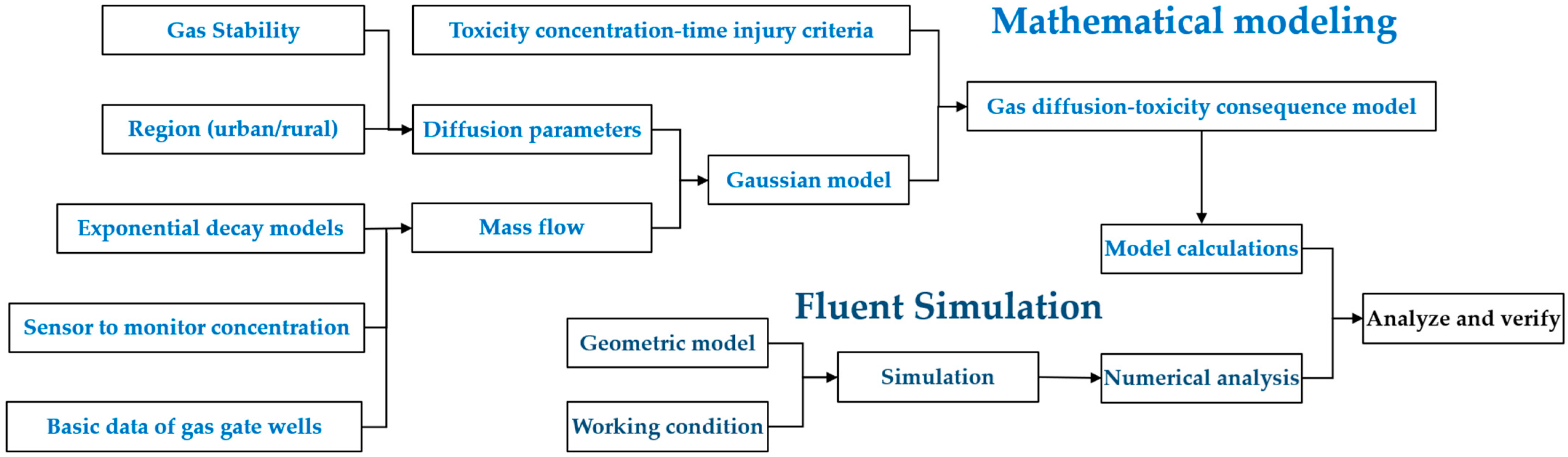
2. Gas Gate Well Leakage Model

The gas gate well is a key facility used in the gas transmission and distribution system. It is generally composed of valves, monitoring instruments, control devices, and other equipment. The gate well is used for the commissioning, maintenance, and repair of gas pipelines (Figure 2). Among the monitoring instruments, concentration monitoring sensors are commonly used to monitor the gas concentration in the gate well. The sensors include natural gas (methane) sensors, liquefied petroleum gas (propane, butane, etc.) sensors, and carbon monoxide sensors. These sensors are characterized by their high sensitivity and fast response, enabling them to detect gas leaks or concentration exceedances in a timely manner and trigger an alarm system to safeguard the safety of personnel.

2.1. Gas Leakage Mass Flow Calculation

The gate well leakage process initially occurs within the well, initiating the diffusion of the gas released from the leakage source. The diffusion of gas within the well is influenced by factors such as the well temperature and gas flow. As the leakage persists, a portion of the gas gradually escapes into the atmosphere through the gate well exit. In the atmosphere, the gas undergoes further diffusion, facilitated by atmospheric layer flow, wind speed, and the surrounding environment.

The gas leakage mass flow rate serves as the foundation for estimating the diffusion range of the leaked gas. In the case of internal methane leakage in the gate well, the gas rapidly diffuses within the well and overflows through the well cover hole. During this stage, the well cover hole can be considered as a leakage source for calculating the mass flow rate of the leaked gas. The mass flow rate of the leakage source is determined by the gas concentration within the well. The gas concentration variation within the well can be observed and monitored using a gas concentration sensor. This paper proposes the use of an exponential attenuation model to fit the gas concentration variation within the well.

The exponential decay model [20] is a mathematical model that describes the exponential decrease in a physical quantity over time. In this model, the rate of change of the physical quantity is directly proportional to its current value, indicating that the rate of decrease is also proportional to the current value. The general form of the exponential decay model for gas concentration discussed in this paper is expressed as follows:

$$C=k{e}^{-\frac{t}{a}}+b$$

(1)

where, a, k, b denotes exponential decay model coefficients, C denotes the methane mole fraction, and t denotes gas leakage time, s.

The model coefficients can be obtained by substituting the gas concentration sensor monitoring data into the model and then predicting the change of concentration in the well after a period of time. The mass flow rate of gas leaking from the gate can be calculated based on the basic information of the pipeline, the basic information of the gate well, and the predicted gas concentration in the gate well.

When a small hole leakage occurs in a gas pipeline, the gas flow at the leakage point is divided into critical flow and subcritical flow, and the calculation formulas for leakage rates differ in these two states. The flow state at the leakage point is determined by the critical pressure ratio, which is the ratio of the critical pressure to the stagnation pressure. The stagnation pressure and critical pressure are fixed values representing the pressure when the gas flow reaches stagnation and critical states, respectively. Therefore, the critical pressure ratio is a constant value [21].

$$\beta =\frac{p_r}{p_t}={\left(\frac{2}{\gamma +1}\right)}^{\frac{\gamma }{\gamma -1}}$$

(2)

where, $\beta$ denotes critical pressure ratio, $p_r$ denotes the critical pressure, and $p_t$ denotes the stagnation pressure.

If $\frac{P_a}{P}\le \beta ,$ the flow state at the leakage point is critical flow. At this time, the mass flow rate of gas at the valve well outlet is:

$$Q=\frac{∆tAP\sqrt{\frac{\gamma }{RT}{\left(\frac{2}{\gamma +1}\right)}^{\frac{\gamma }{\gamma -1}}}-\rho \left(SH+v\right)\left(k{e}^{-\frac{∆t}{a}}+b\right)}{∆t}$$

(3)

If $\frac{P_a}{P}>\beta$, the flow state at the leak point is subcritical flow, and the mass flow rate of gas at the valve well outlet is:

$$Q=\frac{∆tA\frac{P}{\sqrt{RT}}\sqrt{\frac{2\gamma }{\gamma -1}\left({\left(\frac{P_a}{P}\right)}^{\raisebox{1ex}{$2$}\!\left/ \!\raisebox{-1ex}{$\gamma $}\right.}-{\left(\frac{P_a}{P}\right)}^{\raisebox{1ex}{$\gamma +1$}\!\left/ \!\raisebox{-1ex}{$\gamma $}\right.}\right)}-\rho \left(SH+v\right)\left(k{e}^{-\frac{∆t}{a}}+b\right)}{∆t}$$

(4)

where Q denotes the gas mass flow rate at the gate wellhead, kg/s, P denotes the gas internal pressure, Pa, A denotes the leakage hole area, m², T denotes the static temperature, K, R denotes the gas constant, J/(kg·K), $\gamma$ denotes the gas adiabatic index, 1.29, S denotes the valve well surface area, m², H denotes the valve well depth, m, $\rho$ denotes the methane density, kg/m³, v denotes the partial volume of the downhole valve chamber, m³, $∆t$ denotes the predicted leak time, s, and $P_a$ denotes the atmospheric pressure, Pa.

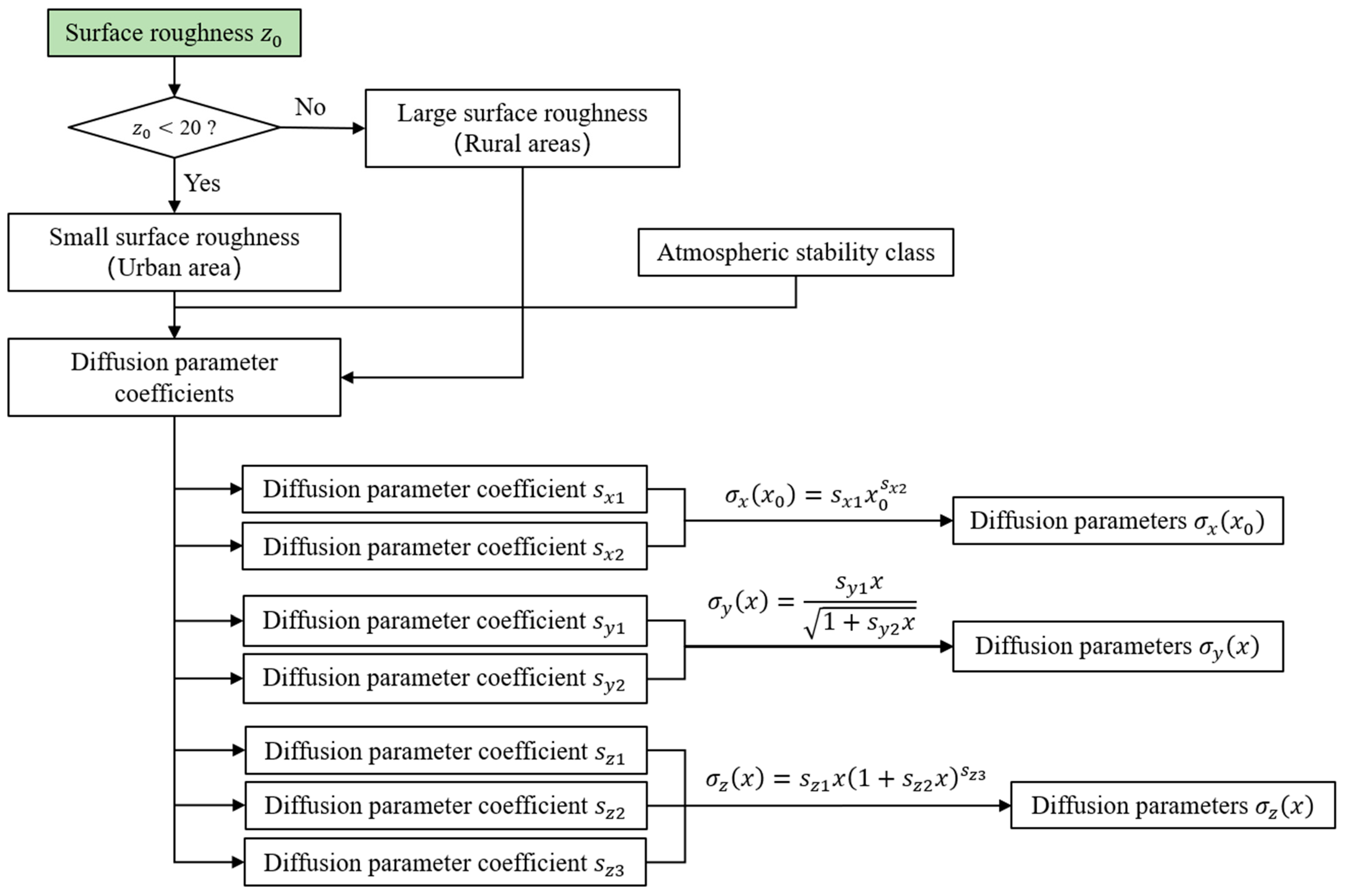
2.2. Calculation of Atmospheric Dispersion Discretization Parameters

The formula for the Gaussian distribution of concentrations in this paper is derived from three empirical diffusion parameters, while the discrete parameters primarily depend on the atmospheric stability class. Pasquill [19] defined six atmospheric stability classes (commonly known as Pasquill–Gifford–Turner stability classes), as shown in

Table 1. Atmospheric stability scale.

Wind Velocity	Illuminance			Cloudiness
	Intense	Moderate	Mild	≥50%	<50%
$U<2$	A	B	B	E	F
$2\le U<3$	B	B	C	E	F
$3\le U<5$	B	C	C	D	E
$5\le U<6$	C	C	D	D	D
$U\ge 6$	C	D	D	D	D

. Classes A through F represent varying degrees of atmospheric turbulence. Class D represents neutral stable conditions, while classes A, B, and C denote unstable conditions. Specifically, Class A represents extremely unstable, Class B represents moderately unstable, and Class C represents slightly unstable. On the other hand, Classes E and F represent progressively stable gas conditions.

The diffusion parameter coefficients can be determined based on the gas stability level and the surface roughness, as illustrated in

Table 2. Reference table for diffusion parameter coefficients.

Surface Roughness	Coefficient	Atmospheric Stability Scale
		A	B	C	D	E	F
Small surface roughness (Rural areas) and Large surface roughness (Urban areas)	$s_{x1}$	0.02	0.02	0.02	0.04	0.17	0.17
	$s_{x2}$	1.22	1.22	1.22	1.14	0.97	0.97
	$s_{y1}$	0.22	0.16	0.11	0.08	0.06	0.04
	$s_{y2}$	0.0001	0.0001	0.0001	0.0001	0.0001	0.0001
Small surface roughness (Rural areas)	$s_{z1}$	0.2	0.12	0.08	0.06	0.03	0.016
	$s_{z2}$	0	0	0.0002	0.0015	0.0003	0.0003
	$s_{z3}$	0	0	−0.5	−0.5	−1	−1
Large surface roughness (Urban areas)	$s_{z1}$	0.24	0.24	0.2	0.14	0.08	0.08
	$s_{z2}$	0.001	0.001	0	0.0003	0.0015	0.0015
	$s_{z3}$	0.5	0.5	0	−0.5	−0.5	−0.5

. Using these coefficients, the diffusion parameters can be calculated. The calculation process is outlined in Figure 3.

2.3. Gas-Diffusion Toxicity Consequence Modeling Based on Gaussian Modeling

In this paper, the utilized gas gate well leakage diffusion model is a Gaussian model that relies on atmospheric diffusion. The computational model for the Gaussian diffusion is presented in

Table 3. Gaussian computational model.

Parameter	Mathematical Expression	Symbol Description	References
Diffusion parameters	${\sigma }_y\left(x\right)=\frac{s_{y1}x}{\sqrt{1+s_{y2}x}}$	$s_{y1}, s_{y2},s_{z1}, s_{z2}, s_{z3}:$ Diffusion parameter coefficients;	[22,23]
	${\sigma }_z\left(x\right)=s_{z1}x{\left(1+s_{z2}x\right)}^{s_{z3}}$	${\sigma }_y\left(x\right):$ Diffusion parameters in the y-direction; ${\sigma }_z\left(x\right):$ Diffusion parameters in the z-direction; $x:$ Coordinates of the target point along the downwind direction with respect to the leakage source.
Concentration at target point	$C\left(x, y, z\right)=\frac{22.4 \times {10}^6}{16.043}\left(\frac{Q}{U}\right)\frac{1}{\sqrt{2\pi }{\sigma }_y\left(x\right)}{e}^{-\frac{1}{2}{\left(\frac{y}{{\sigma }_y\left(x\right)}\right)}^2}\frac{2e^{-\frac{1}{2}{\left(\frac{z}{{\sigma }_z\left(x\right)}\right)}^2}}{\sqrt{2\pi }{\sigma }_z\left(x\right)}$	$Q$: Mass flow rate of gas leakage, (kg/s); $U:$ wind speed, (m/s); $C\left(x, y, z\right):$ The gas concentration at the target point x, y, z; $y:$ Vertical coordinates of the target point relative to the leak source in the downwind direction; z: Vertical coordinates of the target point in the downwind direction relative to the leak source.

. This model is capable of describing the gas leakage behavior under steady-state conditions. To enhance the gas diffusion-toxicity consequence model, the Gaussian diffusion model is integrated with the assessment criterion for toxic concentration injury.

Both domestically and internationally, the toxic concentration injury criterion, or the toxic concentration-time injury criterion, is commonly employed to categorize the extent of impact caused by toxic gas leakage incidents. The Emergency Response Plan Guidelines (ERPG), established by the American Industrial Hygiene Association (AIHA), are presently the recommended standards for exposure concentration. These guidelines have been widely adopted to assess the severity of a toxic gas spill [24,25]. The guidelines specify three concentration ranges, which are outlined in

Table 4. Exposure concentration reference standards.

Concentration	Hazard Level	Result
ERPG-1	I	At this concentration, the general population, including susceptible persons, will experience significant discomfort and some asymptomatic non-sensory effects after 1 h of exposure.
ERPG-2	II	Exposure to this concentration for 1 h resulted in moderate, transient health damage and reduced fugitive ability in the general population, including susceptible populations.
ERPG-3	III	Exposure to this concentration for 1 h causes irreversible, severe, and persistent health damage to humans.

.

In this model, a continuous gas leakage process is simulated using a steady-state leak that lasts for one hour. The gas diffusion-toxicity consequence model is developed based on the toxic concentration-time injury criterion. The calculation model for this is provided in

Table 5. Calculation model of gas diffusion-toxicity consequences.

Hazard Distance	Mathematical Expression	Symbol Description
$x_1$	$C\left(x_1, 0, 0\right)$ $=\frac{22.4 \times {10}^6}{16.043}\left(\frac{Q}{U_{10}}\right)g_y\left(x_1, 0\right)g_z\left(x_1, 0\right)$ $=65000$	$x_1:$ The hazardous area for methane spreading (class I)—the furthest distance to the accident source (m).
$x_2$	$C\left(x_2, 0, 0\right)$ $=\frac{22.4 \times {10}^6}{16.043}\left(\frac{Q}{U_{10}}\right)g_y\left(x_2, 0\right)g_z\left(x_2, 0\right)$ $=230000$	$x_2:$ The hazardous area for methane spreading (class II)—the furthest distance to the accident source (m).
$x_3$	$C\left(x_3, 0, 0\right)$ $=\frac{22.4 \times {10}^6}{16.043}\left(\frac{Q}{U_{10}}\right)g_y\left(x_3, 0\right)g_z\left(x_3, 0\right)$ $=400000$	$x_3:$ The hazardous area for methane spreading (class III)—the furthest distance to the accident source (m).

.

3. Simulation to Analyze and Validate

3.1. Fluent Simulation

ANSYS Fluent (2021R1) is widely used fluid dynamics simulation software developed by ANSYS. It offers a wide range of modeling and solving options, ensuring high accuracy and stability. Due to its popularity and reliability, it is one of the most favored pieces of software for fluid simulation in various fields worldwide [26]. Therefore, for the purposes of this paper, Fluent software was selected for simulation and modeling verification.

3.1.1. Theoretical Modeling and Basic Control Equations

Since methane is the main component of natural gas, it is used instead of natural gas for simulation analysis in this article. To simplify the solving process, the following assumptions are made: the leaked methane and the air inside the valve chamber are considered incompressible ideal gases, and the gas before and after mixing satisfies the ideal gas state equation; the pipeline pressure remains constant during the leakage process, meaning that the leakage aperture and velocity do not change with time; and no chemical reaction occurs between methane and air during the process of methane leakage and diffusion.

By using the PISO algorithm to solve the N-S equations, considering the non-steady-state time term and the influence of gravity and buoyancy, the initial temperature of the gas leak is 288 K and the temperature inside the gate well is 300 K. The standard k-ε equation is selected as the turbulence model, and the component transport equation without chemical reaction is used. The leak hole is set as the velocity outlet boundary condition, the well cover hole is set as the free outflow boundary condition, and the others are wall boundary conditions. Considering the accuracy, stability, and computational efficiency of the simulation, a time step of 0.01 is set.

In this case, the solution method for the convection–diffusion problem is to treat the mass, momentum, energy, and other conservation equations of the diffusing gas in the diffusion region as control equations and to use discrete numerical methods to obtain the distribution law of the mass fraction of the diffusing gas. When considering the solution of the convection–diffusion problem with turbulence, in addition to the basic equations of fluid motion, the convection–diffusion control equations need to be combined. The model control equations are shown in

Table 6. Model control equations.

Governing Equation	Mathematical Expression	Symbol Description
Continuity equation	$\frac{\partial \rho }{\partial t}+div\left(\rho u\right)=0$	$\mathit{div}(-), grad(-)$: vector symbol; $\mathit{div}\left(a\right)=\frac{\partial a_x}{\partial x}+\frac{\partial a_y}{\partial x}+\frac{\partial a_z}{\partial z};$ $gard\left(b\right)=\frac{\partial \mathrm{b}}{\partial x}+\frac{\partial \mathrm{b}}{\partial x}+\frac{\partial b}{\partial z};$ $\rho :$ density, (kg/m3); $t:$ time, (s); $u:$ fluid velocity, (m/s); $u_{i,j,k}:$ component of flow velocity in x, y, z, directions, (m/s); $p:$ fluid pressure, (Pa); $k_0:$ fluid heat transfer coefficient, (W/(m2·K)); $T:$ temperature, (°C); $S_T:$ viscous dissipative term; $c_s$: gas volume concentration, (%); $S_s$: mass per unit time passing through the unit area, (kg); $D_s:$ component diffusion coefficient.
Momentum conservation equation	$\frac{\partial \left(\rho u_{i,j,k}\right)}{\partial t}+\mathit{div}\left(\rho u_{i,j,k}\mu \right)=div(\mu \cdot grad)-\frac{\partial p}{\partial x}+S_{u,v,w}$
Energy conservation equation	$\frac{\partial \left(\rho T\right)}{\partial t}+\mathit{div}\left(\rho uT\right)=div(\frac{k_0}{c_p}·gradT)+S_T$
Component volume transport equation	$\frac{\partial \left(\rho c_s\right)}{\partial t}+\mathit{div}\left(\rho u{c}_s\right)=\mathit{div}(D_s·grad\left(\rho c_s\right))+S_s$
Turbulence control equations	$\begin{array}{c}\frac{\partial \left(\rho k\right)}{\partial t}+\frac{\partial \left(\rho k{u}_x\right)}{\partial x_i}=\\ \frac{\partial }{\partial x_j}\left[\right({\alpha }_k{\mu }_{eff}\left)\frac{\partial k}{\partial x_j}\right]+G_k+G_b-\rho \epsilon -Y_M\end{array}$	$G_k:$ the turbulent kinetic energy induced by the mean velocity gradient; $G_b:$ the turbulent kinetic energy induced by the buoyancy effect; $Y_M:$ the effect of compressible turbulent pulsating expansion on the total dissipation rate; $C_{1\epsilon }, C_{2\epsilon }, C_{3\epsilon }:$ empirical constants;
Dissipation rate equation	$\begin{array}{c}\frac{\partial \left(\rho k\right)}{\partial t}+\frac{\partial \left(\rho k{u}_i\right)}{\partial x_i}=\frac{\partial }{\partial x_j}\left[\right({\alpha }_{\epsilon }{\mu }_{eff}\left)\frac{\partial k}{\partial x_j}\right]\\ +C_{1\epsilon }\frac{\epsilon }{k}(G_k+C_{3\epsilon }{G}_b)-C_{2\epsilon }\rho \frac{{\epsilon }^2}{k}\end{array}$	${\alpha }_k:$ the reciprocal of the effective Prandtl number of the turbulent kinetic energy; ${\alpha }_{\epsilon }:$ the inverse of the effective Prandtl number for the dissipation rate.

[27].

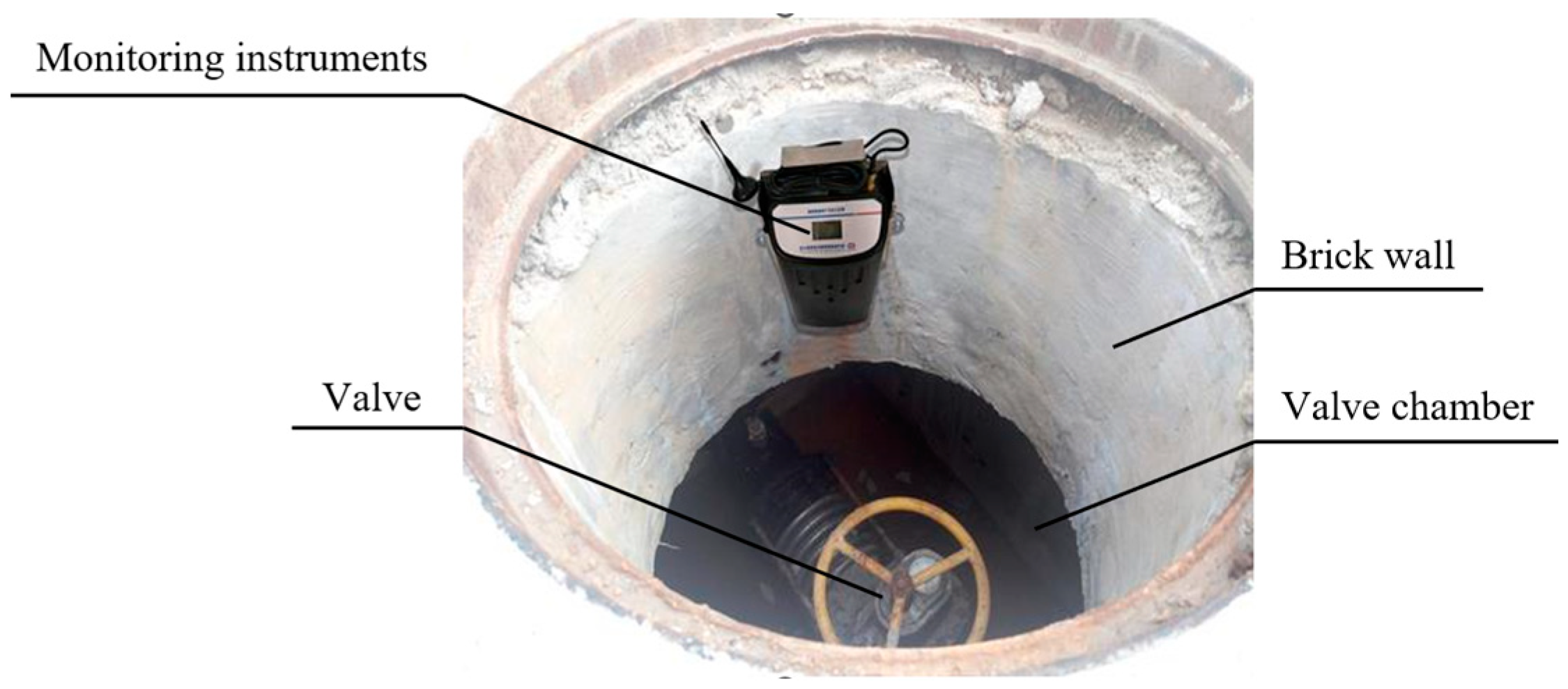
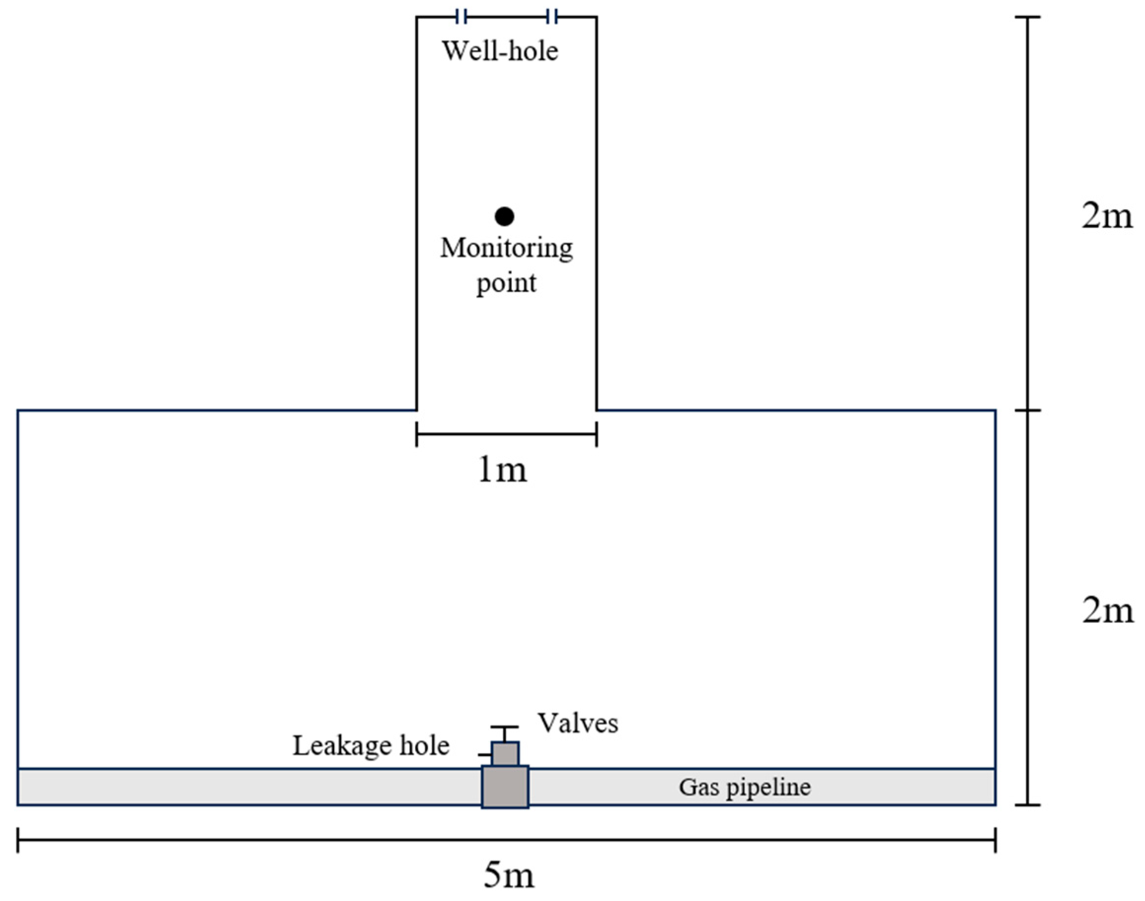
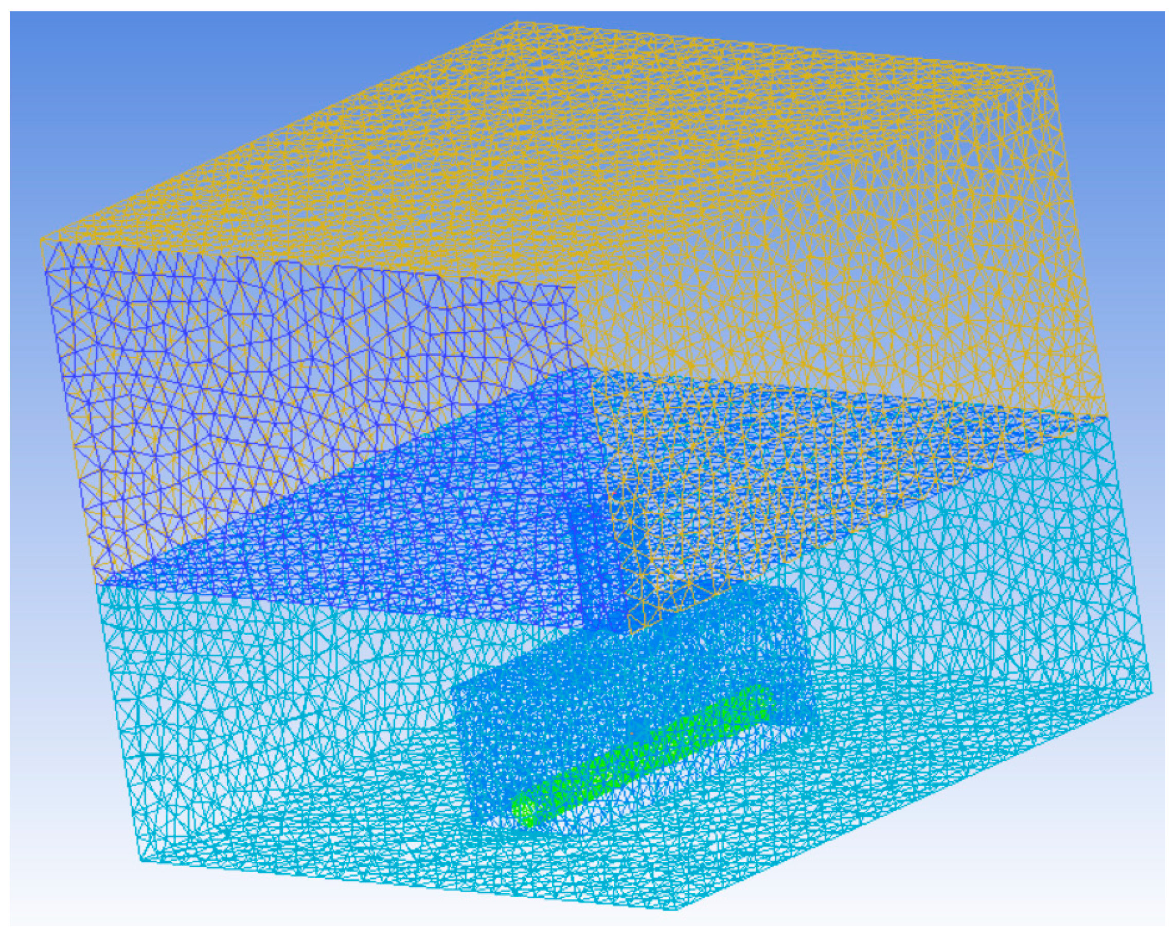
3.1.2. Geometric Modeling

This study focuses on a gas gate well in a large city. The gate well has a depth of 4 m, with the valve chamber below the soil being 2 m deep. The gas transmission pipeline is exposed outside and is 5 m long with a diameter of 0.25 m. It is located at the bottom of the gate well. There is a valve measuring 0.3 m × 0.25 m at the center of the pipeline. The well cover has two round holes with a diameter of 4 cm to allow communication with the atmosphere. A gas concentration monitor is installed 1 m below the well cover. The leakage location in the gate well is often random, but most leakage accidents are caused by poor sealing on the side of the valve. Therefore, the leakage hole is set to the left side of the valve. The internal structure of the gate well can be seen in Figure 4. The area above the well is considered the air domain. To ensure accurate calculations, a large geometric model of the air domain is established to ensure that natural gas can fully diffuse within the air domain. Thus, the size of the entire computational domain is set to 10 m × 10 m × 9 m. The three-dimensional physical model of the gas gate well is shown in Figure 5.

Import the geometric model into the ICME-CFDs software (v.2021R1) for mesh generation. The mesh division of the model directly affects the convergence of simulation results and the computational time. If the mesh is too sparse, it may lead to computational failure, while a mesh too dense will increase the computational difficulty. Generally, considering the significant changes in the flow field near the leak point, a finer mesh is used, while a sparser mesh is used away from the leak point where the pressure gradient is smaller. According to the division results from the ICEM-CFDs software, there are a total of 281,075 mesh cells and 48,002 nodes, as shown in Figure 6.

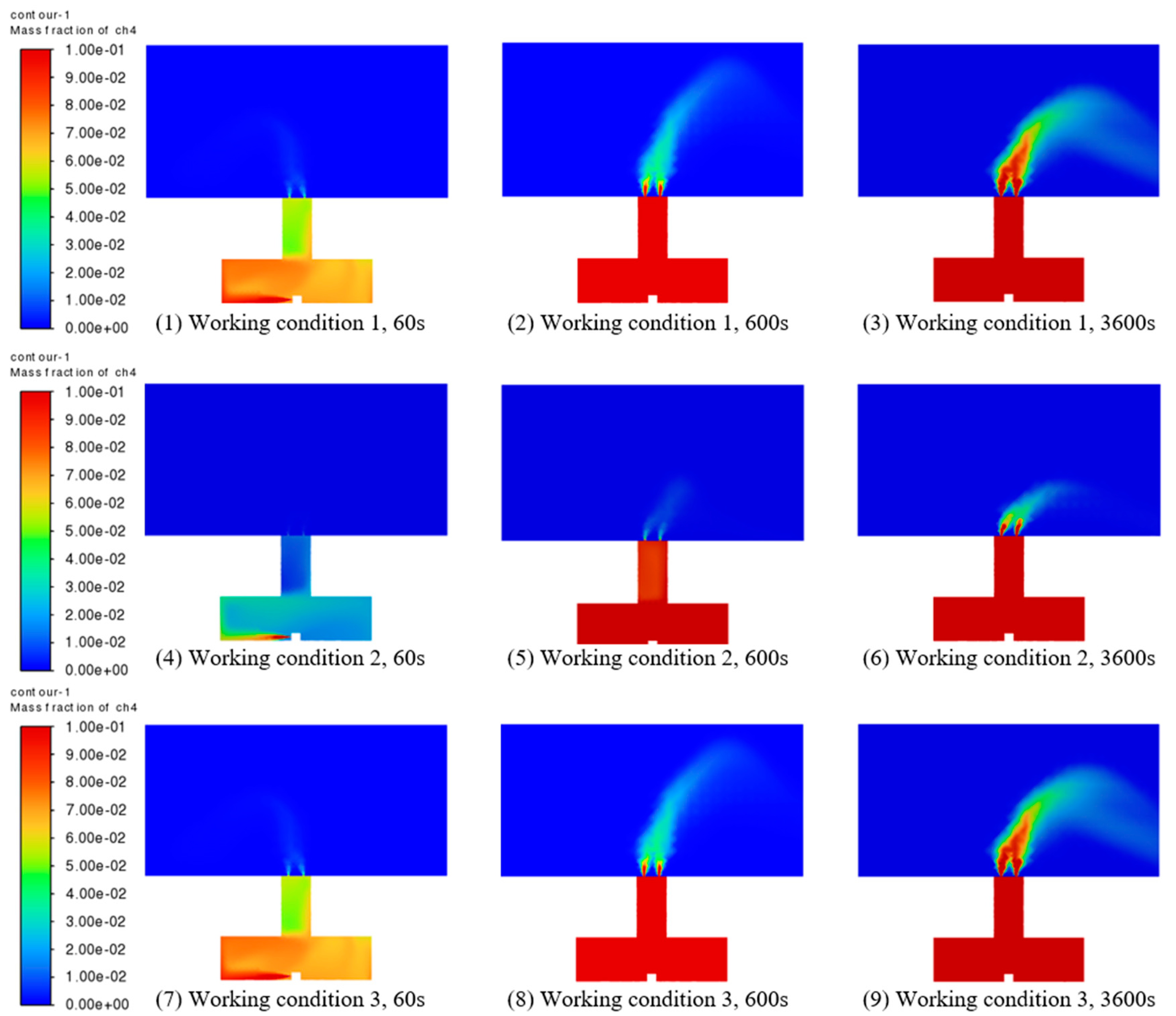
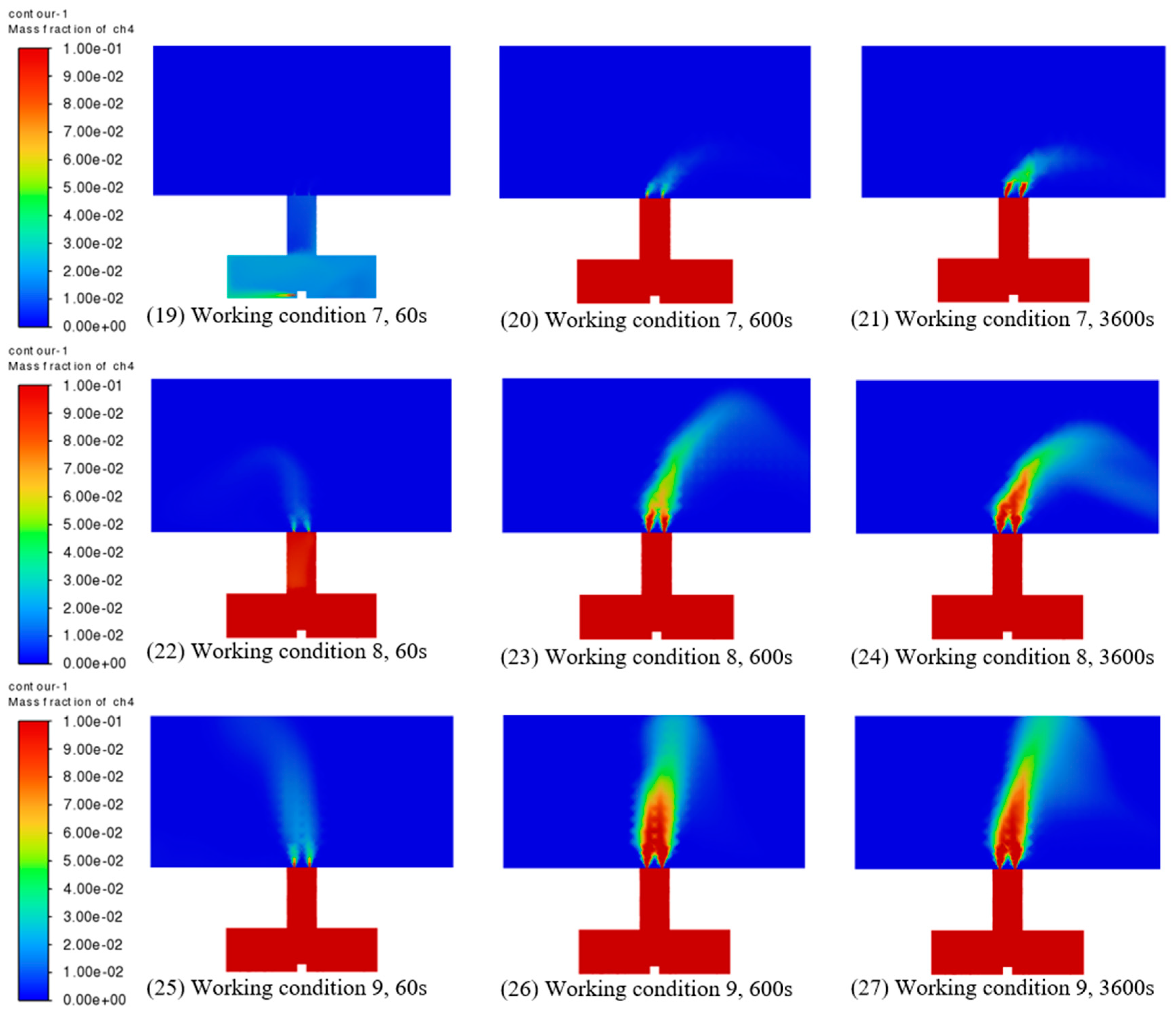
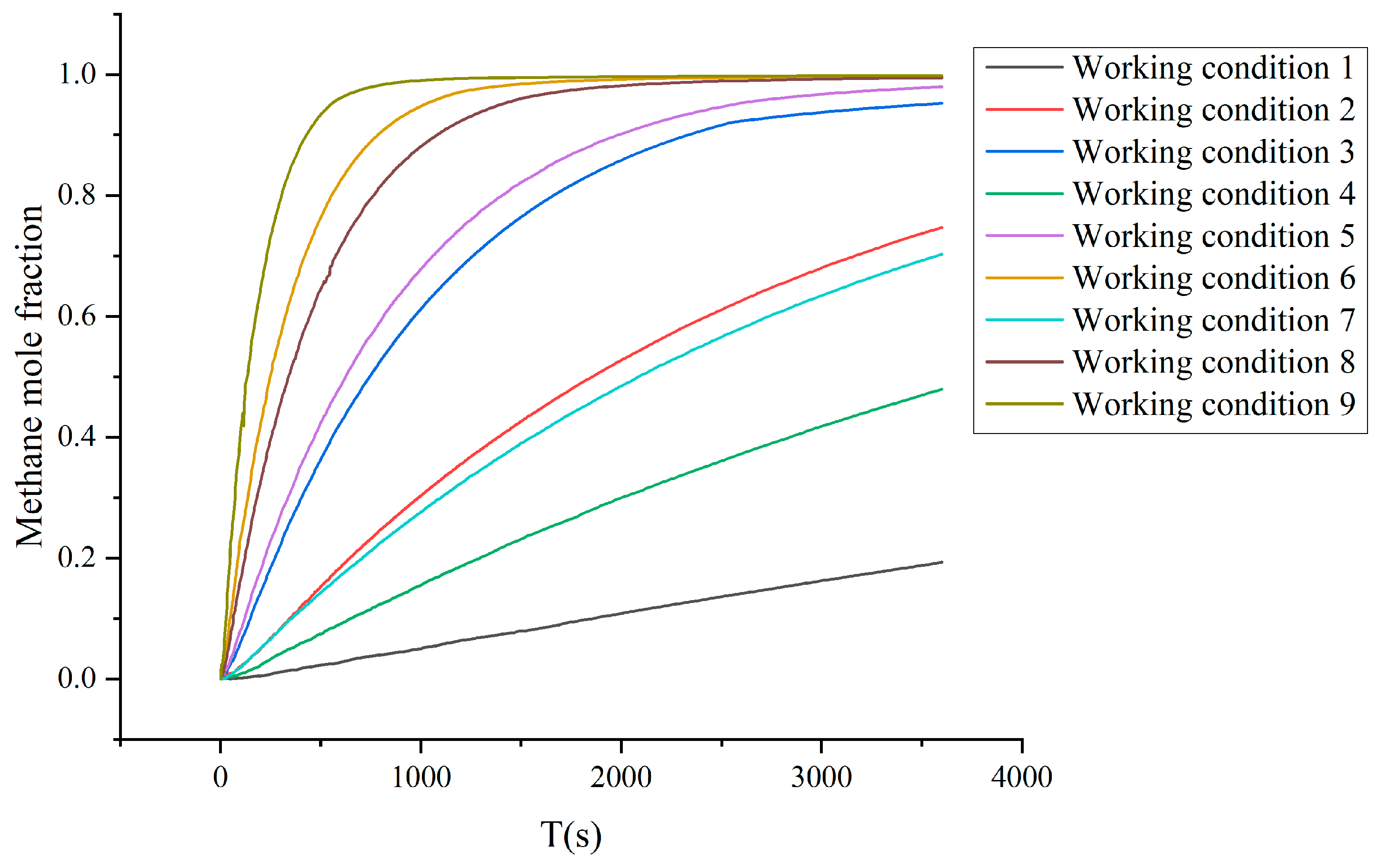
3.1.3. Setting of Working Conditions

Based on the sensitivity analysis of the simulation, we have identified the three factors that have the greatest impact on the diffusion range of the leaked gas. They are wind speed, leak aperture, and pipeline pressure. Based on the analysis results, we have further determined the operating conditions, as shown in

Table 7. Working conditions.

Working Condition	Pipeline Name	Pipeline Pressure (MPa)	Leakage Hole Diameter (mm)
1	Low-pressure gas pipeline	0.009	4
2	Low-pressure gas pipeline	0.009	8
3	Low-pressure gas pipeline	0.009	16
4	Medium-pressure gas pipeline	0.3	4
5	Medium-pressure gas pipeline	0.3	8
6	Medium-pressure gas pipeline	0.3	16
7	High-pressure gas pipeline	1.8	4
8	High-pressure gas pipeline	1.8	8
9	High-pressure gas pipeline	1.8	16

[28].

(1)

Wind Speed: Through sensitivity analysis, we have found that wind speed has a significant influence on the diffusion range of the leaked gas. As the wind speed increases, the diffusion range of the gas also increases, but the danger range caused by the gas leak decreases rapidly. Methane, as a low-density gas, is highly susceptible to atmospheric turbulence. If the atmospheric stability is poor, the gas will not accumulate in a local area due to the influence of wind speed but will be quickly diluted into the surrounding environment, resulting in a significant decrease in the concentration of the leaked gas and a decrease in the danger distance of gas diffusion. Therefore, in the event of a gas valve leakage, the diffusion danger distance will be the farthest under the most stable atmospheric conditions, so we set the wind speed to 0 m/s.

(2)

Aperture: Aperture refers to the diameter of the leak source or nozzle. Through sensitivity analysis, we have also found that the aperture has a significant influence on the diffusion range of the leaked gas. As the aperture increases, the diffusion range also increases. This is because a larger aperture allows more gas to flow through, resulting in the gas diffusing to a wider area. According to the European Gas Pipeline Incident Data Group (EGIG) classification, gas leak models are classified into small-hole models, large-hole models, and pipeline models. Small-hole models are used for calculating leaks when the diameter or equivalent diameter of the leak hole is less than 2 cm. In practical engineering, small-hole leaks have the highest probability of occurrence, while large-hole leaks and pipeline leaks are relatively less common. Therefore, based on the classification standards of the European Gas Pipeline Incident Data Group (EGIG) and the applicable conditions of our model, we simulated and analyzed leaks with diameters of 4 mm, 8 mm, and 16 mm [29].

(3)

Pipeline Pressure: Pipeline pressure refers to the gas pressure inside the pipeline where the leak source is located. Through sensitivity analysis, we have found that pipeline pressure also has a significant impact on the diffusion range of the leaked gas. As the pipeline pressure increases, the diffusion range also increases. This is because higher pipeline pressure leads to a higher leak rate, causing the leaked gas to spread more rapidly to the surrounding space. Gas pipeline pressure levels are generally divided based on the purpose and design parameters of the pipeline. Common pressure levels include low-pressure gas pipelines, medium-pressure gas pipelines, and high-pressure gas pipelines, as shown in

Table 8. Pressure classification of urban gas pipelines.

Pipeline Name	Pressure (MPa)
Low-pressure gas pipeline	$P<0.01$
Medium-pressure gas pipeline	$0.01<P\le 1.6$
High-pressure gas pipeline	$1.6<P\le 4.0$

. Therefore, in this study, we performed simulations with pipeline pressures of 0.009 MPa, 0.3 MPa, and 1.8 MPa.

3.1.4. Simulation Results Analysis

The concentration distribution of gas gate well leakage diffusion over time is depicted in Figure 7 under different working conditions. Initially, when the gas starts to leak from the well, it possesses a large amount of kinetic energy due to the high pressure in the pipeline. This causes the gas to be ejected horizontally, forming a distinct gas column. However, as the gas disperses, it encounters air resistance and friction, causing it to rapidly spread in all directions. The top of the pipe corridor acts as an obstruction, leading to lateral diffusion on the right side of the leakage hole. Some of the gas, under the influence of buoyancy, rises to the top of the shaft, while the remaining portion continues to migrate to the right side of the pipe corridor due to its initial kinetic energy. As time progresses, the kinetic energy of the migrating gas gradually diminishes. When the gas mixture, containing various gas components, reaches the top of the gate well, it creates a vortex that disrupts the stability of the gas column. As a result, the gas column outside the gate well gets displaced.

Figure 8 shows the variation curves of the methane concentration with the leakage time at monitoring points under different working conditions, and it can be seen from the figure that the methane concentration is positively correlated with the leakage aperture diameter and pipeline pressure. With the increase in leakage aperture or pipeline pressure, the methane concentration increases. In the initial gas leak diffusion process, the methane concentration rises faster, and then with the passage of time, the rate of increase gradually slows down. Eventually, the methane concentration increases until it approaches 1.

3.2. Data Verification

The simulation results have been fitted using the exponential decay model of gas concentration, and the corresponding fitted parameters and coefficients of determination for different operating conditions are presented in

Table 9. Model fitting parameters and coefficients of determination for different working conditions.

Working Condition	b	k	a	R2
1	−4237.533 ± 1649.873	4237.528 ± 1649.873	−7.637 × 107 ± 2.973 × 107	0.9992
2	1.044 ± 0.003	−1.062 ± 0.003	2796.381 ± 12.824	0.9995
3	0.998 ± 18.697 × 10−4	−1.028 ± 8.643 × 10−4	1025.049 ± 2.291	0.9994
4	1.134 ± 0.007	−1.143 ± 0.006	6413.479 ± 47.673	0.9997
5	1.003 ± 4.882 × 10−4	−1.028 ± 5.359 × 10−4	871.955 ± 1.187	0.9995
6	0.998 ± 2.327 × 10−4	−1.032 ± 5.379 × 10−4	338.816 ± 0.378	0.9996
7	1.029 ± 0.001	−1.041 ± 0.001	3091.213 ± 6.731	0.9998
8	0.998 ± 2.401 × 10−4	−1.028 ± 4.641 × 10−4	465.728 ± 0.484	0.9998
9	0.996 ± 1.589 × 10−4	−1.028 ± 5.922 × 10−4	183.691 ± 0.207	0.9996

. In statistics and regression analysis, the correlation coefficient (R) is used to measure the degree of linear correlation between two variables. The value of R ranges from −1 to 1, where −1 represents a perfect negative correlation, 1 represents a perfect positive correlation, and 0 indicates no linear relationship. R is commonly employed to assess the goodness of fit of a model. The coefficient of determination, denoted as R squared (R²), is the square of R and signifies the proportion of variation in the dependent variable (explained variable) that can be explained by the independent variable (explanatory variable). R² ranges from 0 to 1, with a value closer to 1 indicating a better fit of the model to the data [30].

Based on the information provided in Table 9, it can be observed that the coefficient of determination R² is consistently above 0.99. This indicates that the fitted gas concentration decay model in the paper aligns well with the simulated gas concentration results in the gate wells. The similar trends and values obtained under different operating conditions further reinforce the accuracy and credibility of the model. Overall, the high degree of accuracy and credibility suggest that the fitted model provides reliable predictions of gas concentration in the gate wells.

Based on the operating conditions, the atmospheric stability level is set to F, and the surface roughness of the area is set to urban surface roughness. By inputting sensor monitoring data, basic information of the gas valve well, geographical location information, and gas leak operating conditions into the gas valve well leak model, we can calculate the farthest distance from different danger levels to the leak source.

Based on the simulated gas leak concentration cloud map and the determined concentration threshold, the concentration contour lines are extracted. Based on the shape and size of the contour lines, the farthest distance from the leak point can be estimated.

The relative error between the calculation results of this model and the Fluent simulation results is shown in

Table 10. The furthest distance of gas leakage spreading hazardous area under different working conditions.

Working Condition	Hazard Level	Hazard Distance—Model Prediction (m)	Hazard Distance—Simulation (m)	Relative Error
1	I	0.43	0.35	0.23
	II	0.11	0.16	0.31
	III	0.05	0.07	0.29
2	I	1.97	1.73	0.14
	II	1.09	1.25	0.13
	III	0.72	0.59	0.22
3	I	2.33	2.27	0.03
	II	1.32	1.62	0.19
	III	0.88	0.91	0.03
4	I	0.96	1.09	0.12
	II	0.49	0.66	0.26
	III	0.18	0.23	0.21
5	I	2.19	2.58	0.15
	II	1.54	1.33	0.16
	III	0.87	0.67	0.32
6	I	2.99	3.22	0.07
	II	1.68	1.87	0.11
	III	1.01	1.12	0.10
7	I	1.16	1.33	0.13
	II	0.55	0.76	0.28
	III	0.26	0.34	0.24
8	I	3.16	3.21	0.02
	II	2.42	2.18	0.11
	III	1.57	1.44	0.09
9	I	4.63	4.85	0.05
	II	2.99	2.88	0.04
	III	2.02	1.98	0.02

.

From the table, it is evident that the average relative error between the predicted data of the model in this paper and the simulated data from the Fluent simulation is 0.15. This indicates that the model exhibits high accuracy and meets the requirements for practical applications.

4. Conclusions

Based on the comprehensive analysis of the research methodology, findings, potential applications, contributions, and limitations, the following conclusions can be drawn.

• The article establishes a gas leak consequence model for gas gate wells by using a Gaussian model and combining time-concentration toxicity standards. It predicts the farthest hazardous distance under different hazard levels based on the predicted gas leak concentration. Compared to traditional simulation methods, this model has a faster calculation speed and can provide timely support in urgent situations. Additionally, this model combines toxicity standards to accurately assess the potential impact of gas leaks on the surrounding environment and human health, thereby assisting emergency responders in better planning and executing response strategies.
• This article proposes, for the first time, the use of an exponential decay model to fit the gas concentration of well leaks. The results show that the gas concentration model for gate wells fits well with the Fluent simulation results, with a coefficient of determination (R²) above 0.99. This means that we can quickly and accurately assess the gas leaks in wells using this model, providing important support for emergency decision making. The proposed research provides a new model approach for predicting gas leak concentrations in wells, offering new ideas and methods for related studies. Other researchers can further explore and improve based on this model to enhance the accuracy and response capabilities of gas leak predictions, thus better ensuring the safety of personnel and the environment.
• By comparison, the average relative error between the gas gate well leakage model predictions and Fluent simulation data in this article is 0.15, indicating a certain feasibility and accuracy in practical application. Compared to Fluent simulation, the gas gate well consequence prediction model in this article is simpler, faster, and more economical. It provides rapid and accurate support for accident emergency response.
• This article studies the mass concentration distribution of gas diffusion based on the Gaussian plume model. The model is suitable for predicting gas diffusion under stable conditions and can accurately predict the diffusion range of leaked gas. However, this model is not applicable to transient gas diffusion caused by instantaneous leakage. In actual situations, the diffusion of gas immediately after a leak is often closely related to factors such as instantaneous flow rate and ejection velocity, which cannot be accurately predicted by steady-state diffusion models. To better address transient gas diffusion from leaks, future research can integrate fluid dynamics methods and numerical simulation techniques to conduct more comprehensive studies. For example, computational fluid dynamics methods can be used to simulate factors such as instantaneous flow rate and ejection velocity and then be combined with the Gaussian plume model to obtain more accurate predictions of concentration distribution. Furthermore, the influence of different environmental conditions and gas properties on gas diffusion needs to be further considered. Factors such as wind speed, temperature, and humidity may have significant impacts on the gas diffusion process. Therefore, introducing complex environmental factors into the model and making corresponding adjustments and corrections will help improve the prediction accuracy and applicability of the model.
• This study, based on the Gaussian model, explores the risks associated with gas pipeline leaks and holds significant implications for sustainable development. It has the potential to promote energy security, reduce environmental pollution, enhance social safety, and facilitate sustainable energy development. Gas pipeline leaks can result in energy wastage, environmental contamination, and safety hazards. By conducting leakage risk prediction and early warning, accurate data and recommendations can be provided to assist relevant departments in formulating practical pipeline maintenance and management strategies, ensuring sustainable energy supply and safe utilization. This research holds great importance in terms of environmental protection, social safety, and the sustainable development of the gas industry.

References

1. Badida, P.; Balasubramaniam, Y.; Jayaprakash, J. Risk evaluation of oil and natural gas pipelines due to natural hazards using fuzzy fault tree analysis. J. Nat. Gas Sci. Eng. 2019, 66, 284–292. [Google Scholar] [CrossRef]
2. Broere, W. Urban underground space: Solving the problems of today’s cities. Tunn. Undergr. Space Technol. 2016, 55, 245–248. [Google Scholar] [CrossRef]
3. Wang, X.; Tan, Y.; Zhang, T.; Zhang, J.; Yu, K. Diffusion process simulation and ventilation strategy for small-hole natural gas leakage in utility tunnels. Tunn. Undergr. Space Technol. 2020, 97, 103276. [Google Scholar] [CrossRef]
4. Li, F.; Wang, W.; Xu, J.; Dubljevic, S.; Khan, F.; Yi, J. A CAST-based causal analysis of the catastrophic underground pipeline gas explosion in Taiwan. Eng. Fail. Anal. 2020, 108, 104343. [Google Scholar] [CrossRef]
5. Zhao, L.; Qi, G.; Dai, Y.; Ou, H.; Xing, Z.; Zhao, L.; Yan, Y. Integrated dynamic risk assessment of buried gas pipeline leakages in urban areas. J. Loss Prev. Process Ind. 2023, 83, 105049. [Google Scholar] [CrossRef]
6. Sun, L.G.; Zhou, Y.W. Study on the leakage pattern of buried gas pipeline network and its secondary disaster prevention. Gas Heat 2010, 30, 38–42. [Google Scholar]
7. Ebrahimi-Moghadam, A.; Farzaneh-Gord, M.; Arabkoohsar, A.; Moghadam, A.J. CFD analysis of natural gas emission from damaged pipelines: Correlation development for leakage estimation. J. Clean. Prod. 2018, 199, 257–271. [Google Scholar] [CrossRef]
8. Bu, F.; Liu, Y.; Wang, Z.; Xu, Z.; Chen, S.; Hao, G.; Guan, B. Analysis of natural gas leakage diffusion characteristics and prediction of invasion distance in utility tunnels. J. Nat. Gas Sci. Eng. 2021, 96, 104270. [Google Scholar] [CrossRef]
9. Li, H.; Feng, H.; Chi, Q. Temperature field simulation of buried natural gas pipeline leakage. Shandong Chem. Ind. 2021, 50, 145–149. [Google Scholar]
10. Yan, Y.T.; Zhang, H.R.; Li, J.M.; Lu, L. Simulation study on leakage diffusion of medium-pressure natural gas pipeline. China Prod. Saf. Sci. Technol. 2014, 10, 5–10. [Google Scholar]
11. Wang, W.; Mou, D.; Li, F.; Dong, C.; Khan, F. Dynamic failure probability analysis of urban gas pipeline network. J. Loss Prev. Process Ind. 2021, 72, 104552. [Google Scholar] [CrossRef]
12. Peng, W.; Zhang, J.; Yuan, H.Y.; Fu, M. Numerical simulation of the effect of leakage holes on gas leakage in deeply buried pipelines. China Prod. Saf. Sci. Technol. 2020, 16, 59–64. [Google Scholar]
13. Zhang, P.; Lan, H. Effects of ventilation on leakage and diffusion law of gas pipeline in utility tunnel. Tunn. Undergr. Space Technol. 2020, 105, 103557. [Google Scholar] [CrossRef]
14. Parvini, M.; Gharagouzlou, E. Gas leakage consequence modeling for buried gas pipelines. J. Loss Prev. Process Ind. 2015, 37, 110–118. [Google Scholar] [CrossRef]
15. Liu, A.; Huang, J.; Li, Z.; Chen, J.; Huang, X.; Chen, K.; Bin Xu, W. Numerical simulation and experiment on the law of urban natural gas leakage and diffusion for different building layouts. J. Nat. Gas Sci. Eng. 2018, 54, 1–10. [Google Scholar] [CrossRef]
16. Zhang, H.; Ma, G.Y. Numerical simulation of leakage diffusion of buried natural gas pipeline under building conditions. J. Liaoning Univ. Petrochem. Technol. 2018, 38, 33–39. [Google Scholar]
17. Li, Y.Z. Numerical Simulation of Urban Commercial Natural Gas Pipeline Leakage and Its Explosion Research. Ph.D. Thesis, Liaoning University of Petrochemical Technology, Fushun, China, 2020. [Google Scholar]
18. Bang, B.H.; Park, C.; Yoon, S.S.; Yarin, A.L. Numerical modeling for turbulent diffusion torch of flammable gas leak from damaged pipeline into atmosphere. Process Saf. Environ. Prot. 2023, 173, 934–945. [Google Scholar] [CrossRef]
19. Pasquill, F. Atmospheric Diffusion, the Dispersion of Windborne Material from Industrial and Other Sources; Ellis Horwood Limited: Chichester, UK, 1962. [Google Scholar]
20. Kwak, S.; Ham, S.; Hwang, Y.; Kim, J. Estimation and prediction of the multiply exponentially decaying daily case fatality rate of COVID-19. J. Supercomput. 2023, 79, 11159–11169. [Google Scholar] [CrossRef]
21. Bu, F. Study on the Diffusion Hazard Law of Multi-Stage Coupled Leakage of Buried Gas Pipeline. Ph.D. Thesis, Northeast Petroleum University, Daqing, China, 2022. [Google Scholar]
22. Liu, C.; Zhou, R.; Su, T.; Jiang, J. Gas diffusion model based on an improved Gaussian plume model for inverse calculations of the source strength. J. Loss Prev. Process Ind. 2022, 75, 104677. [Google Scholar] [CrossRef]
23. Snoun, H.; Krichen, M.; Chérif, H. A comprehensive review of Gaussian atmospheric dispersion models: Current usage and future perspectives. Euro-Mediterr. J. Environ. Integr. 2023, 8, 219–242. [Google Scholar] [CrossRef]
24. Cavender, F.; Phillips, S.; Holland, M. Development of emergency response planning guidelines (ERPGs). J. Med. Toxicol. 2008, 4, 127–131. [Google Scholar] [CrossRef] [PubMed]
25. Griffiths, S.D.; Entwistle, J.A.; Kelly, F.J.; Deary, M.E. Characterising the ground level concentrations of harmful organic and inorganic substances released during major industrial fires, and implications for human health. Environ. Int. 2022, 162, 107152. [Google Scholar] [CrossRef] [PubMed]
26. Mei, Y.; Shuai, J. Research on natural gas leakage and diffusion characteristics in enclosed building layout. Process Saf. Environ. Prot. 2022, 161, 247–262. [Google Scholar] [CrossRef]
27. He, F. Principles and Applications of CFD Software for Computational Fluid Dynamics Analysis; Tsinghua University Press: Beijing, China, 2023. [Google Scholar]
28. Code for Urban Gas Design (with Explanatory Notes), 2002 ed.; Ministry of Construction of the People’s Republic of China: Beijing, China, 2002.
29. Wang, Y.T.; Lu, Y.X.; Yang, W.L.; Sun, X.; Zhu, X.X. A review of domestic and international research on gas pipeline accidents. Chem. Equip. Pip. 2022, 59, 78–84. [Google Scholar]
30. Chen, H.Y. (Ed.) Statistics; Beijing Institute of Technology Press: Beijing, China, 2021. [Google Scholar]
Figure 1. Research roadmap for this paper.
Sustainability 16 00091 g001
Figure 2. Gas gate well site construction plan.
Sustainability 16 00091 g002
Figure 3. Flow chart for calculation of diffusion parameters.
Sustainability 16 00091 g003
Figure 4. Two-dimensional physical model of the internal structure of the gate wells.
Sustainability 16 00091 g004
Figure 5. Three-dimensional physical model of a gas gate well.
Sustainability 16 00091 g005
Figure 6. Grid division results.
Sustainability 16 00091 g006
Figure 7. Leakage spread of gas gate wells under different working conditions.
Sustainability 16 00091 g007aSustainability 16 00091 g007bSustainability 16 00091 g007c
Figure 8. Change curve of methane concentration at monitoring points under different working conditions.
Sustainability 16 00091 g008