Multilevel Change of Urban Green Space and Spatiotemporal Heterogeneity Analysis of Driving Factors

Abstract

Analyzing the change trend of urban green space (UGS) and exploring related driving forces can provide scientific reference for sustainable development in rapidly urbanizing areas. However, the spatial and temporal driving mechanisms of the drivers on UGS patterns at different scales are still not deeply understood. Based on the GlobeLand30 land cover data, nighttime lighting data and spatial statistics from 2000 to 2020, this study analyzed the size, shape and diversity of UGS in Guangzhou at the urban level, gradient level and township level with multiple landscape indices. Diversity means the richness of UGS patch types. The selected indices include percent of landscape (PLAND), largest path index (LPI), landscape shape index (LSI), aggregation index (AI) and Shannon’s diversity index (SHDI). The spatiotemporal heterogeneity of the drivers was then explored using the spatiotemporal weighted regression (GTWR) method. Results showed the following: (1) During 2000−2020, the total amount of UGS in Guangzhou increased slightly and then decreased gradually. UGS was mainly transferred into artificial surfaces (lands modified by human activities). (2) The UGS landscape showed a non-linear trend along the urban–rural gradient and fluctuated more in the interval of 20–60% urbanization level. PLAND, LPI and AI decreased significantly in areas with higher levels of urbanization. LSI increased and SHDI decreased significantly in areas with lower levels of urbanization. At township level, the landscape indices showed significant spatial autocorrelation. They transformed from discrete changes at the edge and at the junction of the administrative district to large-scale aggregated change, especially in northern areas. (3) The size of UGSs was mainly influenced by natural factors and population density, but their shape and diversity were mainly influenced by socio-economic factors. More regular shapes of green patches were expected in higher urbanization areas. Population agglomeration positively influenced green space patterns in the northeastern and southern regions (Zengcheng, Conghua and Nansha). Meanwhile the negative influence of urban expansion on the green space pattern in the central and southern regions decreased over time. This study contributes to an in-depth understanding of how the key factors affect the different changes of UGS with time and space and provides methodological support for the long-term zoning planning and management of UGS.

1. Introduction

Urban green space (UGS), as an natural public space and ecological welfare, plays an important role in improving the quality of the ecological environment [1,2,3], promoting the physical and mental health of citizens [4,5] and sustaining urban vitality [6]. In the context of rapid global urbanization, UGSs are undergoing rapid changes, especially in developing countries [7,8]. The contradiction between UGS and construction land is gradually intensifying [9]. Therefore, timely monitoring of UGS dynamics and scientific management and planning of UGS system are of great importance for the sustainable development of cities.

In 1898, Ebenezer Howard proposed the “garden city”, emphasizing that urban construction should use large green space to reduce urban density in order to create a beautiful and livable living environment [10]. This concept elaborates the idea that urban development should be coordinated with UGS, which makes UGS regarded as an important means to control the growth of urban scale. In the 1990s, countries such as the United States, Brazil and New Zealand gradually incorporated UGS planning as an organic component of urban development into their master planning systems and promulgated corresponding planning policies to regulate management. In the twenty-first century, urbanization has led to environmental degradation and the loss of global biodiversity. This trend is more common in developing countries, and especially in some cities in Asia [11]. As the largest developing country in the world, China is facing a strong conflict between urban development and environmental sustainability [2]. Development is usually preceded by governance. Therefore, we would like to gain a comprehensive understanding of the evolutionary characteristics and related drivers of UGS patterns in rapidly growing megacities at different scales, which are conducive to multi-scale spatial planning and management of UGS. The study of UGS mainly includes the characteristics of UGS pattern, the evolution process, and the driving mechanism, so as to reveal the complex relationship between UGS and other elements of urbanization. In terms of spatial pattern characteristics and evolution processes, most relevant studies are based on remote sensing monitoring data at different time periods, and the spatiotemporal evolution pattern is analyzed from the aspects of area change, land use transfer, landscape pattern, and morphology analysis. The studies pointed out that a full understanding of the pattern of UGS requires multidimensional measurements, as the size and landscape pattern of the UGS exhibits different trends over time [2,12]. For example, Liu et al. compared and analyzed the spatial and temporal evolution characteristics of UGS in terms of size, morphology, spatial layout and greening policies, using Shanghai and Xuchang as examples. Emphasizing the fulfilment of quantitative requirements does not evaluate the rationality, systematicity and stability of the UGS [13]. Moreover, the spatial and temporal evolution of green space varies from one sub-region to another [14]. And the quality and changes in UGS are associated with different levels of cities and stages of urbanization [15]. For example, Wu et al. comparatively analyzed the NDVI changes in green spaces in three zones of the city center, suburbs and the islands of Shanghai. The results showed that intensity of urbanization development significantly affects the UGS change process. Thus, the spatial heterogeneity of UGS changes deserves attention. A growing number of studies have attempted to analyze the dynamics of landscape patterns in the UGS, but fewer have captured the spatially heterogeneous characteristics of UGS changes at different scales, such as the comprehensive analysis of urban level, urbanization gradient and township level, which maybe not conductive to the systematic monitoring of UGS.

The driving forces of UGS distribution and structure are mainly driven by natural geographical factors and human activities [16]. Natural geographical factors, such as average altitude, annual average temperature and precipitation, influence the change in UGS by affecting the distribution, survival and reproduction of vegetation [16,17]. At the same time, the increasing pressure of population on land resources caused by rapid urbanization and the subsequent increase in buildings and infrastructure may be the main reasons for the reduction and fragmentation of UGS [11,18]. Typical urbanization factors include population and land expansion, economic growth and public investment [2]. Urban expansion often occurs on the edge of green space [18]. Xu et al. argued that labor, land, and capital are the main drivers influencing changes in UGS patterns in Chinese cities, and these drivers are spatially heterogeneous [16]. In addition, greening policies have been suggested to be the main driver of UGS recovery [11,19]. Existing studies have used a range of mathematical statistics and spatial statistical models to explore the drivers of variation in UGS dynamics [20], such as correlation analysis [21], stepwise regression analysis [22], generalized linear models (GLM) [15], geodetector [23] and geographically weighted regression (GWR) [24], etc. Among them, geodetector and GWR, as commonly used spatial analysis models, take into account the spatial heterogeneity of variable relationships, and are better able to express complex geographic change processes compared to linear regression methods [23,25]. But they can only investigate the drivers for a single time period [26,27]. In fact, the driving process of vegetation evolution exhibit both spatiotemporal nonstationarity and time lag [28]. Ignoring the unbalanced effects of the time dimension may affect the accuracy of their results [29,30]. Geographically and Temporally Weighted Regression (GTWR) is an extension of the GWR model, which can reflect the spatial and temporal variability of variables by constructing a weight matrix based on spatial and temporal distances, has received increasing attention [26,31]. For instance, Hu et al. used GTWR and MGWR to investigate driving mechanisms of landscape patterns on habitat quality [32]. However, most of the current driving mechanism analyses are mostly focused on changes in area, vegetation index and fragmentation, and the driving mechanism explanations of multi-dimensional UGS dynamics, such as shape and diversity, are slightly insufficient. In addition, most of the studies are based on large-scale spatial analysis units and static data, which are not deep enough to analyze the changes of factor forces in different periods and locations.

Guangzhou is a densely populated and fast-growing economic region in China. Its per capita gross domestic product (GDP) has increased from 25,800 yuan in 2000 to 134,000 yuan in 2020. Rapid urban development in the past 20 years has brought about a contradiction between urban growth and the protection of UGS. How to solve this contradiction and realize sustainable development requires understanding the process of UGS changes in the past, so as to formulate relevant land management policies. In this view, this study took Guangzhou in China as an example, and the evolution of UGS multidimensional patterns was analyzed using the three phases of land cover data from 2000 to 2020. Then, at the street and township scale, we used the spatial and temporal geographically weighted regression (GTWR) model to explore the spatiotemporal heterogeneity of the driving factors. This paper focuses on three questions: (1) How did the size, shape and diversity of UGS in Guangzhou change over time between 2000 and 2020? (2) Spatially, how are changes in the above characteristics distributed at multiple levels? (3) Did the relationships between UGS changes and the corresponding drivers remain stable throughout the city over time? The results are intended to provide theoretical support for the optimization of UGS patterns and the implementation of control measures for different areas in other similar cities, as well as to improve the relevant theories and models of UGS development.

2. Materials and Methods

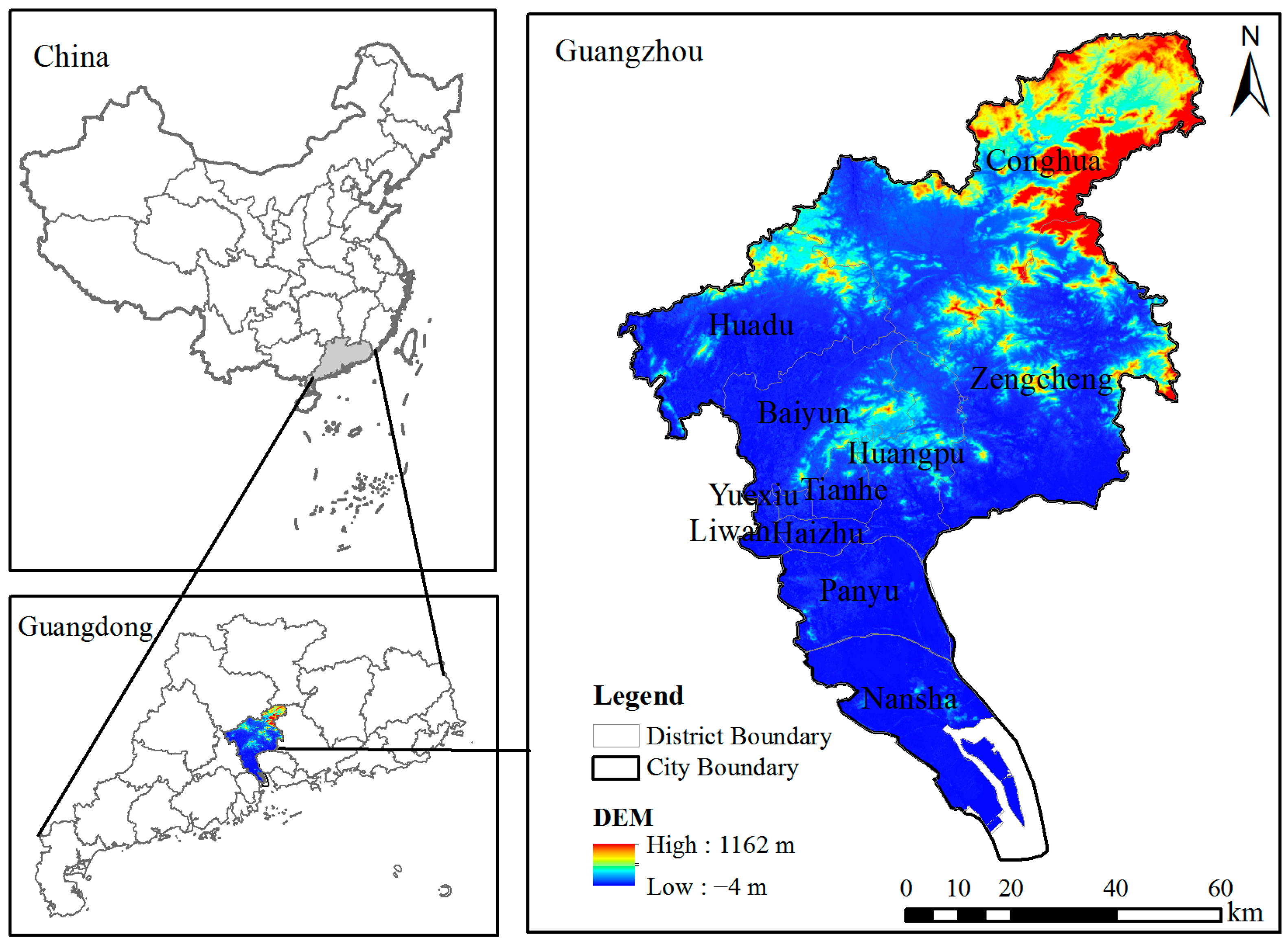
2.1. Study Area

Guangzhou is located in the central and southern part of Guangdong Province (Figure 1). It is one of the most economically developed large cities in China. It has 11 districts, including Yuexiu, Liwan, Tianhe, Haizhu, Baiyun, Huadu, Huangpu, Panyu, Nansha, Conghua and Zengcheng, with a total area of 7434.4 km². Among them, Yuexiu, Liwan, Tianhe and Haizhu are the central areas. By December 2021, Guangzhou could be divided into 142 streets and 34 townships, totaling 176 spatial units. The seventh national census shows that the total population of Guangzhou is 18.67666 million. Guangzhou experiences a southern subtropical monsoon climate, with an annual average temperature between 21.5 °C and 22.2 °C, and it is rich in UGS resources. It is generally high in the north and low in the south, with mountains and high hills in the north and plains and terraces in the south, which are rich in water resources. Because of the complex natural morphology and rapid urbanization, Guangzhou has become a typical area to study the process and driving mechanism of UGS change. The relevant results can serve as a reference for UGS monitoring and zoning planning in other similar cities.

2.2. Data Sources and Processing

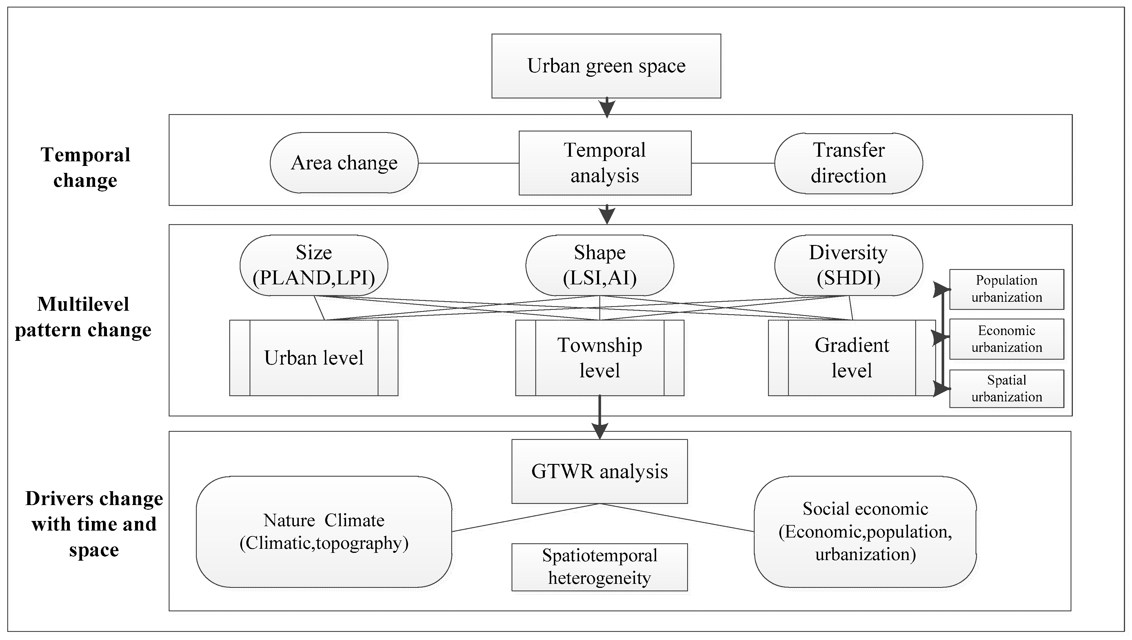
The data mainly include land cover data, natural environment and socioeconomic data. The land cover data were obtained from GlobeLand30 platform for the years 2000, 2010 and 2020 in a 30-m resolution and were reclassified and clipped in ArcMap 10.8 software according to the administrative boundaries of Guangzhou city (https://www.webmap.cn/, accessed on 2 January 2023). The study area mainly contains six original land-cover types, namely cultivated land, forest, grassland, shrubland, water bodies, wetland, artificial surfaces and bareland. Artificial surfaces refer to lands modified by human activities, including all types of residential land, mines and transportation facilities. Referring to the UGS Classification Standard (CJJ/T85-2017) [33] and the purpose of the study, the concept of UGS in this study is land with vegetation characteristics and public space attributes. It consists mainly of natural and man-made green space. We therefore combined forest, grassland and shrubland into one category, represented as UGS. Finally, the GlobeLand 30 land cover data were reclassified into six land cover types: cultivated land, UGS, water bodies, artificial surfaces and unutilized land. Temperature and precipitation data were obtained from the spatially interpolated dataset of average conditions of meteorological elements in China with a spatial resolution of 1 km (https://www.resdc.cn/, accessed on 10 January 2023). Topographic data were derived from 30-m resolution digital elevation model (DEM) data provided by Geospatial data cloud platform (https://www.gscloud.cn/, accessed on 10 January 2023). Socioeconomic data include population density data, gross domestic product (GDP) data and nighttime light data. Population density data, GDP data were both obtained from the Resource and Environment Science and Data center (https://www.resdc.cn/, accessed on 2 March 2023). Because nighttime light data can explore the urbanization process from a spatial perspective, the level of urbanization in each region was assessed using nighttime light data as the independent variable [34]. The nighttime light data were obtained from the improved time-series DMSP-OLS-like data (1992–2022) in China published by Harvard Dataverse (https://dataverse.harvard.edu/, accessed on 10 March 2023). These data were converted to the same projected coordinate WGS_1984_UTM_Zone_49N. Using the ArcGIS clipping tool, the corresponding data was obtained for the range of Guangzhou city. The data of each street and township were obtained by overlaying vector boundary clipping on the original data.

2.3. Methods

Figure 2 represents the framework proposed in this study. The study is divided into three parts, including the temporal change of UGS, the multi-level landscape pattern changes and the spatiotemporal heterogeneity of driving factors. First, changes in the size of the UGS and the direction of transfer were analyzed based on Globeland30 data. Second, changes in landscape patterns were analyzed at the city level, township level and gradient level using landscape indices. Finally, natural climate and socio-economic data were integrated and spatiotemporal geographically weighted regression was used to identify influencing factors at the township street scale.

2.3.1. Landscape Index

Landscape pattern index can reflect the composition and spatial allocation of landscape structure, and quantitatively describe the evolution of landscape pattern and its influence on ecological processes [35,36]. Based on correlative references [35,36], the indicators that represent the overall size, shape and diversity of UGS were selected from the patch and landscape levels. The selected indices include percent of landscape (PLAND), largest path index (LPI), landscape shape index (LSI), aggregation index (AI) and Shannon’s diversity index (SHDI). Among them, PLAND and LPI characterize the proportion and dominance of UGS, LSI and AI indicate the shape complexity and aggregation of UGS, respectively, and SHDI represents the UGS diversity (

Table 1. The description of landscape indicators.

Landscape Indicator	Type	Description
PLAND (Percent of landscape)	Size (Proportion of UGS)	The percentage of a certain patch area in the landscape to the whole landscape area. The larger the value, the greater the proportion of this type area.
LPI (Largest path index)	Size (Dominance of UGS)	The percentage of the largest patch of the corresponding patch type in the landscape. The greater the value, the more concentrated and dominant the landscape is.
LSI (Landscape shape index)	Shape (Morphology of UGS)	The ratio of perimeter to area measures the overall morphological complexity of the landscape. The greater the value, the higher the irregularity of patches and the more complex the landscape shape.
AI (Aggregation Index)	Shape (Aggregation of UGS)	The aggregation index indicates the degree of aggregation between landscape patches. The greater the value, the higher the aggregation degree of the same kind of plaque.
SHDI (Shannon’s Diversity Index)	Diversity (Richness of UGS)	This index can reflect the richness of landscape patch types. The greater value, the richer the landscape types and the stronger the spatial heterogeneity.

). Three-phase raster data at the township scale in Guangzhou were imported by using Fragststs 4.2 software, and each landscape index results in the long time series from 2000 to 2020 were obtained. Metrics were used for two levels of analysis, at the overall and zonal scales. Fragstats 4.2 software was used to calculate the landscape index.

2.3.2. Urbanization Gradient Analysis

Urbanization is a process of change in the socio-economic development in a region. It is specifically manifested in the agglomeration of urban population, the outward expansion of urban areas and the non-agricultural adjustment of industrial and economic structures [37]. With reference to related research [38,39], the gradient of urbanization is comprehensively characterized from three aspects: population urbanization, spatial urbanization and economic urbanization. Among them, the population density characterizes the population urbanization level, the nighttime light index represents the economic urbanization level and the proportion of artificial surface area is used to represent the spatial urbanization level. The above three indicators are normalized and then the average value is calculated to measure the comprehensive development level of urbanization (UDI).

$$UDI=\frac{POD+NTL+ASA}{3}$$

(1)

where UDI is the urbanization development index, POD is the population density, NTL is the nighttime light index, ASA is the proportion of artificial surface area.

2.3.3. Driving Factor Selection

Socio-economic and natural climatic conditions are considered to be the main driving factors affecting the evolution of UGS [2,15,34]. Referring to the relevant literature [2,12,17,34,40,41,42,43], seven factors, as shown in the

Table 2. Influence factors associated with UGS landscapes.

Dimension	Subcategory	Indicator	Abbreviation	Reference
Nature climate	Climatic	Average annual temperature	TEM	[44]
		Annual precipitation	PRE	[2,17]
	Topography	DEM	DEM	[2,17]
Social economic	Economic development	GDP	GDP	[2,17]
	Population concentration	Population density	POD	[2,42]
	Urban expansion	Artificial surface area	ASA	[2,45]
	Urbanization level	Nighttime light	NTL	[34,46]

, were selected to explore the driving mechanism. Among them, average annual temperature (TEM), annual precipitation (PRE) and DEM were used to quantify the climate and topography. GDP, population density (POD), artificial surface area (ASA) and nighttime light (NTL) were used to characterize the level of economy, population and urbanization.

2.3.4. Geographically and Temporally Weighted Regression

Geographically weighted regression (GWR) model can estimate the degree of influence of drivers on different regions; it is an important tool for studying spatial heterogeneity [47]. However, the model only considers the spatial dimension and lacks the examination of the temporal dimension. The GTWR model considers the temporal dimension of the variables by calculating the GWR model, which produces more accurate results in time series analysis [32,46,48]. In this view, the model is used to analyze the spatial heterogeneity of UGS drivers. Its formula is as follows:

$$y_i={\beta }_0\left(u_i,v_i,t_i\right)+{\sum }_{k=1}^p{\beta }_k\left(u_i,v_i,t_i\right)x_{ik}+{\epsilon }_i,$$

(2)

where y is the dependent variable, x_ik is the independent variable, i is the sample area, u_i and v_i are the latitude and longitude of the sample area i, respectively, t_i is the time, β₀(u_i,v_i,t_i) is the intercept, β_k(u_i,v_i,t_i) is the estimation coefficient, k is the explanatory variable number, p is the total number of explanatory variables, β_k > 0 is the positive correlation between the independent variables and the dependent variable, and vice versa, and ε_i is the random perturbation term. This study is based on the “GTWR ADDIN (v1_1_20_May2020)” tool for calculation [31]. Considering the comparability of different indicators, all indicators have been standardized using Z-score.

3. Results

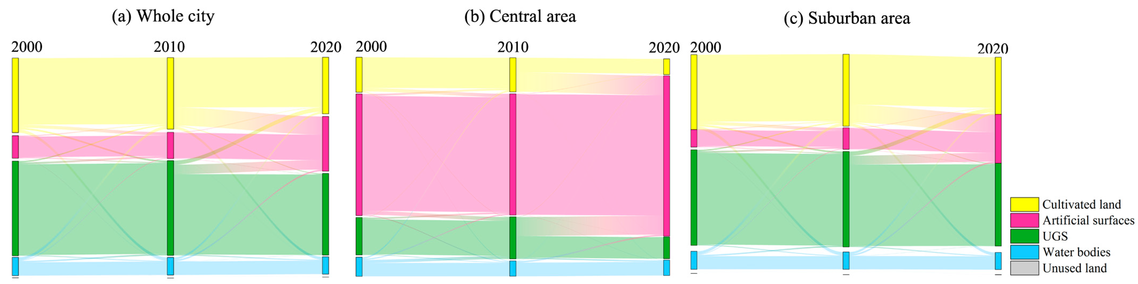
3.1. Temporal Analysis of UGSs

The distribution pattern of UGS in Guangzhou is shown in Figure 3. In 2000, 2010 and 2020, the total area of UGS was 3241.66 km², 3244.32 km² and 2794.35 km², respectively. In terms of quantitative changes, from 2000 to 2010, the area of UGS was stable with a slight increase, with a change rate of 0.08%. However, from 2010 to 2020, the area of UGS decreased significantly, with a change rate of −13.87%. The transfer between UGS and other land cover types is shown in Figure 4. In the whole city and suburbs, UGS transferred mainly into artificial surface and cultivated land, especially from 2010 to 2020. And some of the cultivated land was converted back into UGS. The transfer direction of UGS in the central area was different. The main change of UGS in the central area was the transfer between UGS and artificial surface.

3.2. Landscape Change of UGSs at Multiple Levels

3.2.1. UGS Landscape Change at Urban Level

As shown in

Table 3. Overall statistics of UGS landscape dynamics.

Year	PLAND	LPI	LSI	AI	SHDI
2000	45.032	22.427	54.854	97.160	0.332
2010	45.069	22.541	54.363	97.188	0.341
2020	38.795	16.201	60.297	96.633	0.272

, from 2000 to 2020, PLAND, LPI, AI and SHDI showed a trend of initial gradual increase and then rapid decrease, indicating that the area ratio, dominance, aggregation and diversity of green landscape increased slightly from 2000 to 2010 and decreased rapidly from 2010 to 2020. LSI showed a trend of gradual decline initially and then rapid increase, indicating that the complexity of green landscape shape tends from simple to complex and then irregular. In general, the change rate of UGS landscape index in 2010–2020 was faster than that in 2000–2010, indicating that the degree of human interference became stronger in the subsequent stage.

3.2.2. UGS Landscape Change at Gradient Level

The trend of the landscape indices along the urbanization gradient was shown in Figure 5. The landscape pattern indices exhibited a non-linear trend along the urban–rural gradient. They generally had an obvious inflection point around 20–50% of the comprehensive development level of urbanization, indicating that the UGS landscape in the urban–rural fringe area was highly heterogeneous, and the changes are more complicated.

Comparing different years, the values of PLAND, LPI and AI in 2020 were significantly lower than those in 2000 and 2010 in areas with an urbanization level greater than 40%. This indicated that the size and agglomeration of UGS in areas with higher combined urbanization levels decreased significantly. The values of LSI in 2020 were significantly higher than those in 2000 and 2010 in the interval of less than 70% urbanization level, which indicated that the UGS patches in the area of medium and low urbanization levels became more complicated. The trend of SHDI differed from that of the other indices, increasing in the interval of 0–60% urbanization level and then decreasing in the interval greater than 60%. The overall SHDI value in 2020 was lower than that in 2000 and 2020, especially in the low- and medium-urbanization-level regions.

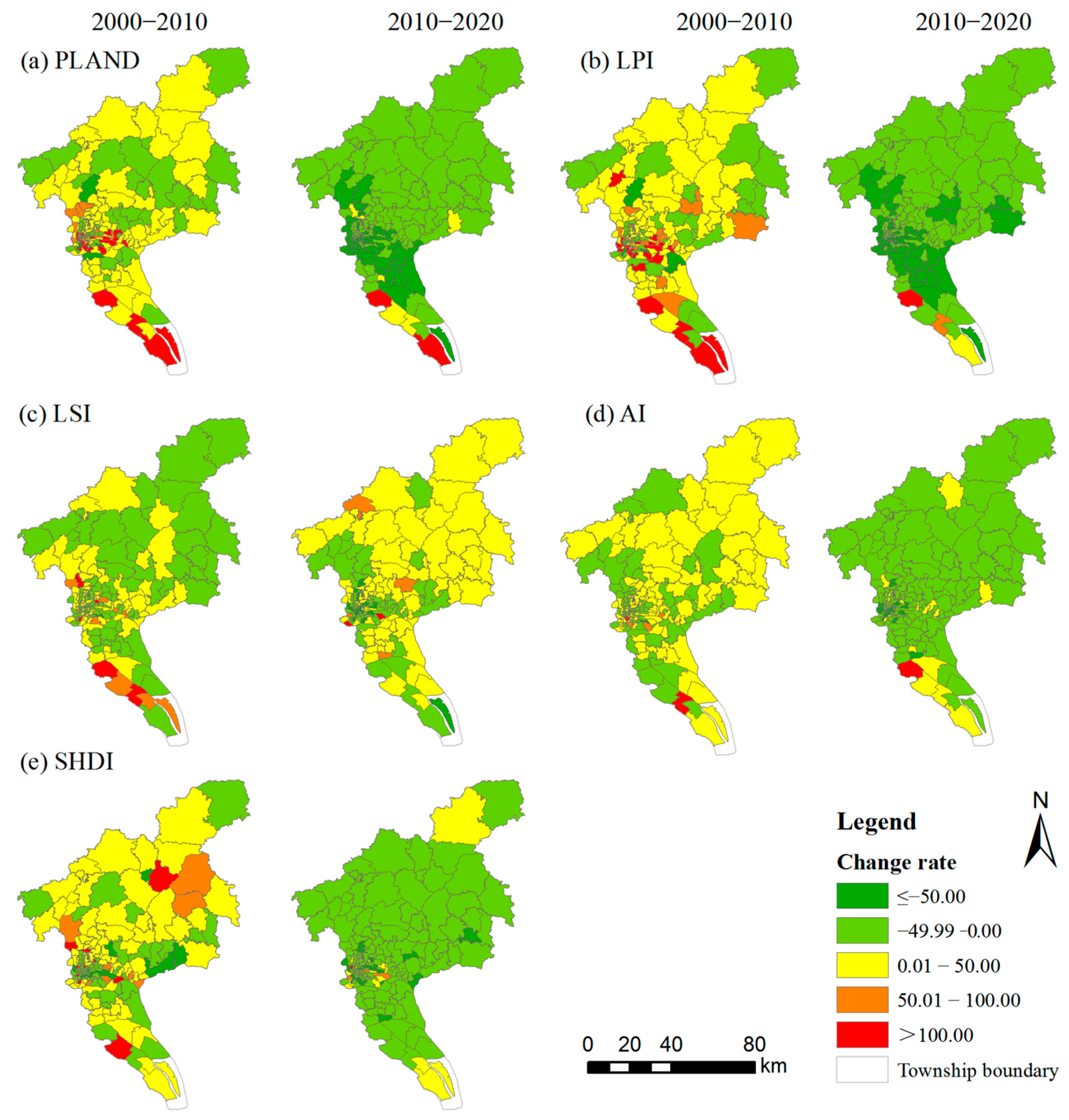
3.2.3. UGS Landscape Change at Township Level

The landscape indices changed from discrete to aggregated changes, and the range of changes expanded significantly (Figure 6). In terms of landscape size, PLAND and LPI decreased significantly from 2000 to 2010 mainly at the edges and junctions of Huadu, Conghua and Nansha. Between 2010 and 2020, the range of decreases gradually migrated southward and eastward, with significant decreases in the central four districts, the northwestern part of the Baiyun district, and the east-central part of the Huangpu district.

In terms of landscape shape, from 2000 to 2010, LSI decreased significantly in the central and eastern parts of Nansha, and the pattern of UGS patches became regular. From 2010 to 2020, it increased significantly in the northern part of the region and the coastal area of Nansha, and the pattern of green space patches became complex. In 2000–2010, AI decreased mainly in the western border and the junction of northern districts. In 2010–2020, the range of decrease spread significantly, and the degree of aggregation decreased in general.

In terms of landscape diversity, the decreasing area gradually changed from a discrete distribution to an aggregated decrease in the central area. From 2010 to 2020, the central area decreased significantly, while the diversity in Liangkou Town of Conghua District and the southern coastal area of Nansha District increased significantly.

3.3. Factors of UGSs Landscape Dynamics Based on GTWR

3.3.1. Spatial Autocorrelation and Collinearity Test

Results showed that each index had a higher spatial autocorrelation in each year, satisfying the requirement of spatial heterogeneity for spatial weighted regression (

Table 4. Spatial autocorrelation statistics of landscape index.

	PLAND			LPI			LSI			AI			SHDI
	2000	2010	2020	2000	2010	2020	2000	2010	2020	2000	2010	2020	2000	2010	2020
Moran’s I	0.611	0.595	0.685	0.494	0.492	0.619	0.721	0.708	0.723	0.446	0.408	0.526	0.447	0.523	0.390
p value	0.001	0.001	0.001	0.001	0.001	0.001	0.001	0.001	0.001	0.001	0.001	0.001	0.001	0.001	0.001

). Then, seven selected driving factors were tested for collinearity and significance. Specifically, the factors corresponding to each landscape index were selected by step-based regression. The results showed that the VIF of each selected factor was less than 7.5, and the p value was less than 0.05, satisfying the requirements of collinearity and significance test (

Table 5. GTWR regression and OLS regression result statistics.

Landscape Index	GTWR R2 Adjusted	OLS R2 Adjusted	Variable	OLS Standardized Regression Coefficient	p Value	Variance Inflation Factor
PLAND	0.752	0.637	DEM	0.606	0.000	1.823
			PRE	0.092	0.001	1.119
			POD	−0.145	0.000	1.226
			NTL	−0.143	0.000	1.998
LPI	0.682	0.584	TEM	−0.101	0.001	1.092
			DEM	0.710	0.000	1.079
			POD	−0.097	0.001	1.132
LSI	0.733	0.698	TEM	0.121	0.001	2.457
			PRE	0.151	0.000	1.788
			GDP	0.081	0.013	1.798
			POD	−0.158	0.000	1.465
			DG	−0.585	0.000	1.253
			ASA	0.327	0.000	1.612
AI	0.414	0.305	PRE	0.231	0.000	1.143
			GDP	0.111	0.014	1.515
			POD	−0.214	0.000	1.388
			NTL	−0.235	0.000	1.253
			ASA	0.167	0.000	1.557
SHDI	0.438	0.188	TEM	−0.159	0.000	1.265
			POD	−0.176	0.000	1.435
			NTL	−0.185	0.001	2.003
			ASA	0.247	0.000	1.254
			DEM	−0.322	0.000	1.768

). Then the selected variables were analyzed using GTWR regression, and the results showed that the corresponding R² is higher than 0.41, indicating that the model had an excellent fit degree. The maximum, minimum and mean absolute values of the regression coefficients are shown in

Table 6. GTWR regression coefficient of the main drivers of landscape index.

Dependent	Variable	Maximum				Minimum				Mean
Variable		2000	2010	2020	2000–2020	2000	2010	2020	2000–2020	2000	2010	2020	2000–2020
PLAND	DEM	4.822	4.104	3.193	4.034	0.224	0.204	0.114	0.202	0.909	0.854	0.854	0.872
	PRE	0.360	0.219	0.203	0.250	−0.219	−0.041	−0.271	−0.098	0.089	0.070	0.067	0.053
	POD	33.626	19.807	19.815	24.416	−12.165	−8.712	−18.576	−13.151	0.898	0.786	0.814	0.826
	NTL	0.069	0.088	0.034	0.028	−2.083	−1.133	−1.403	−1.540	0.390	0.387	0.392	0.389
LPI	TEM	0.091	0.020	−0.029	0.007	−0.702	−0.620	−0.650	−0.655	0.113	0.102	0.138	0.118
	DEM	4.990	4.219	3.127	4.053	0.365	0.412	0.501	0.447	1.006	0.945	0.831	0.927
	POD	67.319	47.204	38.166	50.896	−21.003	−15.868	−21.648	−14.068	1.415	1.155	1.064	1.211
	TEM	0.361	0.341	0.315	0.317	0.039	0.023	0.007	0.023	0.118	0.119	0.104	0.114
LSI	PRE	0.294	0.292	0.257	0.281	−0.258	−0.269	−0.279	−0.269	0.141	0.143	0.124	0.136
	GDP	0.759	0.893	0.792	0.815	−0.081	−0.101	−0.100	−0.094	0.059	0.061	0.067	0.063
	POD	−0.065	−0.089	−0.114	−0.107	−2.028	−5.765	−4.526	−4.106	0.148	0.177	0.179	0.168
	NTL	−0.216	−0.222	−0.232	−0.223	−0.821	−0.768	−0.763	−0.774	0.532	0.530	0.532	0.531
	ASA	0.517	0.490	0.469	0.492	0.171	0.137	0.207	0.182	0.406	0.393	0.380	0.393
	PRE	0.521	0.379	0.424	0.428	0.003	0.003	0.003	0.004	0.318	0.277	0.287	0.294
AI	GDP	0.350	0.274	0.317	0.222	−0.355	−0.176	−0.028	−0.134	0.091	0.119	0.179	0.130
	POD	0.270	0.093	0.472	0.077	−3.621	−1.896	−2.302	−1.573	0.178	0.232	0.342	0.251
	NTL	−0.005	−0.012	−0.007	−0.017	−0.712	−0.708	−0.594	−0.659	0.437	0.373	0.254	0.355
	ASA	0.891	0.599	0.506	0.657	−0.012	−0.010	−0.022	−0.002	0.573	0.331	0.230	0.378
	TEM	0.045	−0.069	0.538	0.060	−1.041	−0.562	−0.754	−0.786	0.133	0.195	0.147	0.158
SHDI	POD	98.009	70.193	60.505	76.236	−4.185	−0.478	−11.902	−5.371	1.173	0.892	0.765	0.943
	NTL	5.918	3.965	3.517	4.467	−0.569	−0.789	−0.549	−0.504	0.396	0.410	0.181	0.329
	ASA	1.470	1.035	0.717	1.074	−0.896	−0.544	−0.510	−0.650	0.902	0.598	0.387	0.629
	DEM	1.139	1.134	1.068	1.114	−1.067	−1.040	−1.328	−0.859	0.369	0.344	0.304	0.339

. The regression coefficients were further used to measure the direction of action of the drivers and the intensity of their influence in terms of time and space.

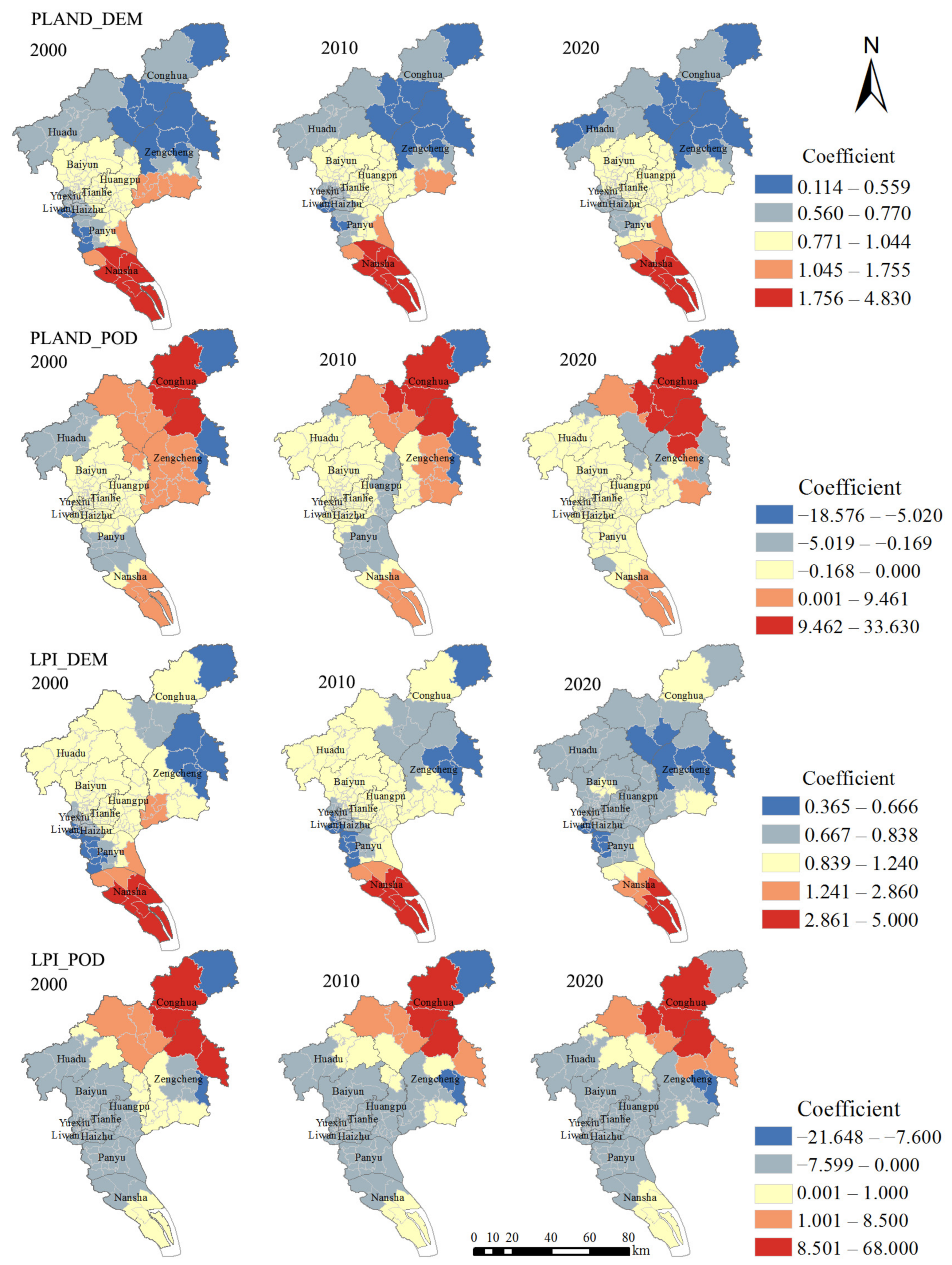
3.3.2. Drivers of the Size of UGSs

The regression results of PLAND showed that from 2000 to 2020, considering the average absolute values of the regression coefficients, the influence degree from high to low was as follows: DEM, POD, NTL and PRE, among which DEM and POD had more significant influence than other factors. DEM had a positive effect on the PLAND of UGS, and the influence degree in 2020 is slightly lower than that in 2000. Spatially, the regression coefficient was higher in the middle and south, and lower in the northeast (Figure 7). In 2020, the range of towns with high influence was reduced. The direction of influence of POD was more complex, and the degree of influence showed a trend of slow weakening and then gradually increasing. Spatially, the result showed a negative impact in the central and western regions, and a positive impact in most areas of Zengcheng, Conghua and Nansha. In addition, the number of townships with negative influence gradually increased. In 2020, POD shifted from positive promotion to negative inhibition on the junction between Zengcheng District and Huangpu District, as well as between Conghua District and Baiyun District and Huangpu District.

The regression results of LPI showed that from 2000 to 2020, the influence degree from high to low was as follows: POD, DEM and TEM, among which POD and DEM had more significant influence than the other factors. POD had a complex influence on LPI of UGS landscape, which was mainly positive in some townships of Zengcheng and Conghua and Nansha District and negative in the central and western regions (Figure 7). During the period from 2000 to 2020, the range of towns with negative impacts expanded, mainly concentrated in the intersection of Zengcheng District and Huangpu District. DEM always had a positive impact on LPI, but the influence degree decreased. Spatially, the regression coefficient gradually increased from the northeast to the south, but its impact on the central and surrounding areas gradually decreased.

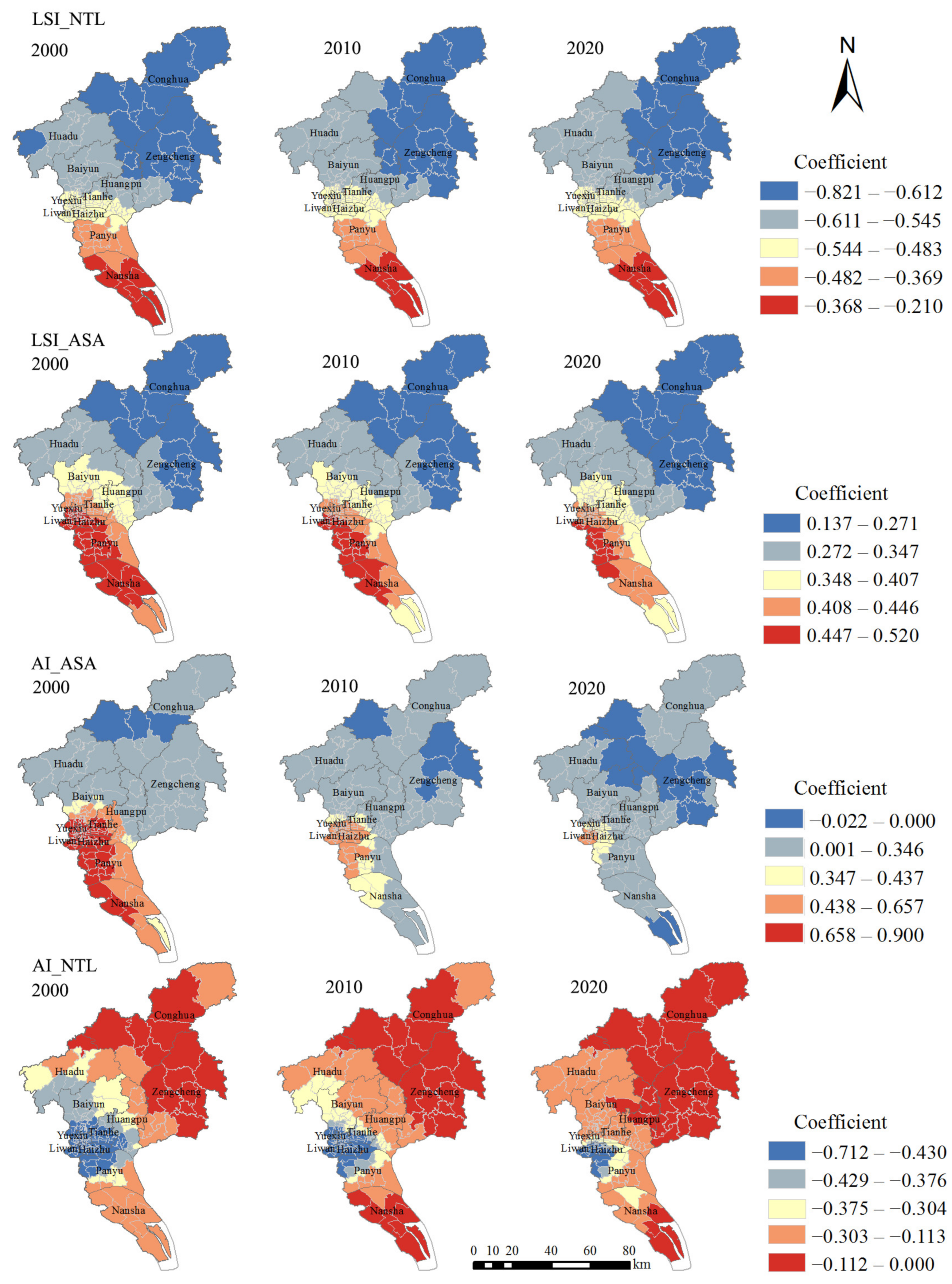
3.3.3. Drivers of the Shape of UGSs

The regression results of LSI showed that from 2000 to 2020, the order of the influence degree from high to low was as follows: NTL, ASA, POD, PRE, TEM and GDP, among which the influence of NTL and ASA was more significant than the other factors. NTL exhibited a negative effect on LSI, suggesting that the larger night light value indicated smaller LSI value. During 2000 to 2020, the degree and range of NTL influence were relatively stable, showing a gradual decreasing trend from northeast to southwest, and the negative effect on Zengcheng district and Conghua district was more significant (Figure 8). This finding showed that the higher light value indicated higher urbanization level, and less complex and regular shape of green patches. ASA had a positive effect on LSI, indicating that the larger construction land range suggested a more complex green landscape form. Spatially, this finding showed a gradual increasing trend from northeast to southwest, mainly affecting the southwestern regions, such as Liwan District, Panyu District and the western part of Nansha District. The influence of ASA in 2020 had weakened compared with that in 2000, and the scope of high influence had gradually narrowed.

The regression results of AI showed that from 2000 to 2020, the influence degree of each factor was ranked from high to low as follows: ASA > NTL > PRE > POD > GDP. ASA showed a more complex influence direction on UGS landscape AI (Figure 8). It had a negative influence on some towns in Conghua and Zengcheng, and the influence scope was gradually expanded, whereas the significant positive influence scope on the central city was gradually reduced. This finding showed that the marginal area was greatly affected by the expansion of construction land, and the concentration of UGS decreased. NTL had a negative impact on landscape AI in UGS, the spatial influence decreased from the central urban area to the outer circle, and the high influence range of NTL gradually decreased during 2000–2020.

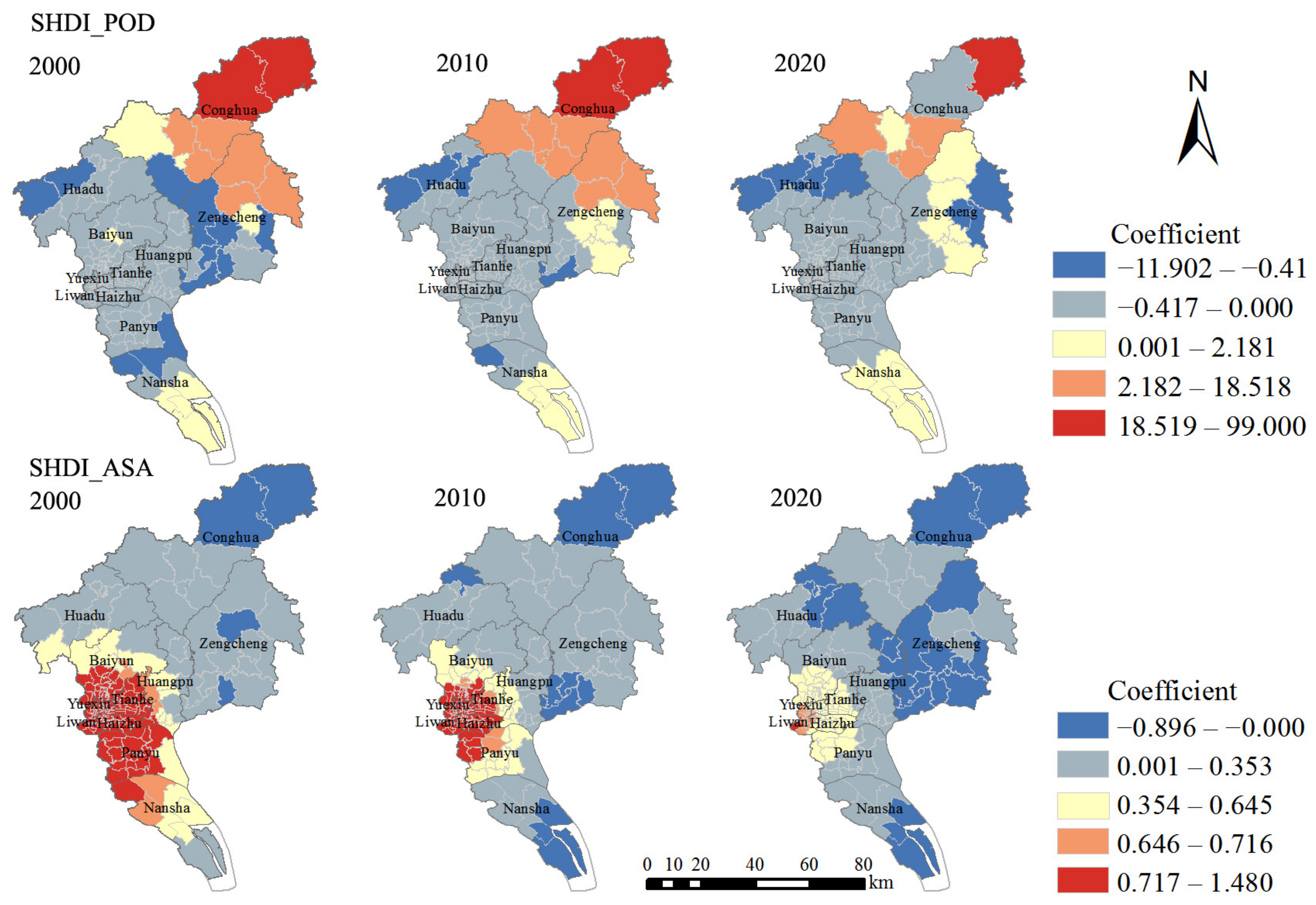
3.3.4. Drivers of the Diversity of UGSs

The results of SHDI regression showed that, from 2000 to 2020, the order of influence degree from high to low was POD > ASA > DEM > NTL > TEM, and POD and ASA had significant influence on the diversity of UGS. POD had a complicated influence on the landscape diversity of UGS (Figure 9). It negatively impacted the central and western regions, but positively affected the northern and southern regions (Zengcheng District, Conghua District and most areas of Nansha District). However, between 2010 and 2020, the scope of positive high influence had decreased. ASA had a positive impact on the central and southern regions, whereas it had a negative impact on the northern region of Conghua, Zengcheng and some southern regions of Nansha. Moreover, from 2010 to 2020, the range of regions with positive high impact decreased, whereas those with negative high impact expanded. This finding showed that the greater population density in the central and western regions indicated lower diversity of UGS. However, in Zengcheng District, Conghua District and some areas of Nansha, the diversity of UGS increased with the concentration of population. At the same time, the expansion of built-up land in suburban areas reduced the diversity of UGS.

4. Discussion

4.1. Multilevel Change of UGSs in Guangzhou from 2000 to 2020

Compared with previous studies, this study extended the research from a single city level to the district level and gradient level, which provides a richer understanding of the temporal and spatial evolution processes of UGS landscapes in Guangzhou. UGS landscape patterns differed spatially and temporally. In the first stage (2000–2010), the overall UGS landscape pattern was slightly optimized. In the second stage (2010–2020), the overall UGS landscape decreased in size, aggregation and diversity, and patch shape became complex. This finding is consistent with the results of related research [49,50]. Spatially, the landscape indices showed significant spatial autocorrelation. They transformed from discrete changes at the edge and at the junction of the administrative district to large-scale aggregated changes. The development of Guangzhou’s urban space expanded eastward along the Pearl River and then extended to the northeast and southeast. Thus, the range of UGS size decrease gradually migrated southward and eastward. Compared to other landscape indices, the distribution of changes in LSI is significantly different. The main reason for this is that the suburbs mainly include natural green landscapes, and the center area mainly comprises man-made green landscapes. Man-made green landscape means artificial occurring landscape features covering a range of green services and facilities that meet local and strategic needs and contribute to a good quality of city life, such as comprehensive parks, pocket parks, etc. Natural green landscape refers to naturally occurring landscapes, such as national park systems and ecological protection forests, etc. [51]. In different urbanization areas, the relationship between landscape pattern index and human disturbance is obviously different [52]. With the intensification of human activities, the shape of man-made green space has gradually become regular, while the shape of natural green space has changed from regular to complex. As a result, the LSI of the UGS in the northern region, which is dominated by natural landscapes, increased between 2010 and 2020. At the gradient level, the landscape index was found to show a non-linear trend along the urban–rural gradient and fluctuated more in the interval of 20–60% urbanization level. This was basically consistent with the results of landscape index changes using concentric circles by Wu et al. [2]. In the urban–rural transition zone, the landscape pattern of the UGS changed dramatically, and some natural landscapes such as grasslands and forests were gradually transformed into urban parks. The urban sprawl and complex land use configuration made the UGS in this area show a highly dynamic and spatially heterogeneous change trend.

4.2. Spatiotemporal Heterogeneity of Natural Socio-Economic Factors

The influence of factors on different landscape characteristics of UGSs may vary with location and time. Geographically weighted regression models (GWR) and temporally weighted regression (TWR) can be used to identify differences in the temporal residual and spatial domains [53,54,55]. However, these models do not simultaneously address the spatial and temporal nonstationarity in variables relationships, which may reduce their precision in modeling the variables of interest. Based on a spatiotemporal perspective, this study used the GTWR model to capture the spatiotemporally varying responses of different UGS landscape characteristics to natural socio-economic factors. It was found that population, artificial surface area, level of urbanization and DEM were the main factors in the evolution of UGS landscapes, and their influence was spatially and temporally heterogeneous.

The size of UGS was mainly influenced by DEM and POD. Overall, DEM had a positive influence. The influence direction of population density was complex, negatively affecting the central and western regions of Guangzhou and positively affecting most towns and villages in Zengcheng, Conghua and Nansha. This finding was consistent with the conclusions of Yu [56] and Wang [57], showing that population gathering does not necessarily bring negative effects to UGS. This is related to the economic growth mode and ecological policies in different areas [17]. Population inflow may promote social cohesion, sustainable lifestyle and green economy, which is conducive to the implementation of greening policy [57,58]. For example, from 2010 to 2020, the average annual growth rate of the population of Nansha Subdistrict is 12.53%. The inflow of population prompted the government to exert efforts in the construction of urban “livable” and improved the construction of projects, such as Huangshan Lu Forest Park, Jiaomen Park, Big Tiger Mountain and Monkey Island Forest Park, Tianhou Palace, Dajiao Mountain Park, Million Sunflower Garden and Wetland eight scenes. Thus, UGS area increased. However, at the junction of the central city and the peripheral city, the range of negative effects of population agglomeration had expanded over time. This finding showed that the outward expansion range of construction land should be reasonably controlled at the edge of the central area. It is recommended that the government should pay attention to the coordination between population growth and urban capacity, and minimize the negative impact of population concentration on the surrounding green environment.

The shape of UGS was mainly influenced by NTL and ASA. The NTL had a positive impact on the morphology of UGS in this area but had a negative impact on the agglomeration of UGS. It showed that as the step of urbanization speeds up, land use becomes more intensive and the spatial structure of cities becomes more regularized [13], so that the morphology of UGS patches tend to become simpler. However, major conflicts between real estate development and UGS protection often lead to UGS reduction and fragmentation [34,57]. In addition, the expansion of artificial surface area exhibited different effects on the aggregation of UGS in the central area and the suburbs. The main reason was that the increase of urban area can provide more space for UGSs within the central area, but it may displace the natural green space, so the UGS agglomeration in the central area increases while that in the suburban area decreased [34,57].

The diversity of UGS was largely influenced by POD and ASA. Population concentration had a negative effect on UGS diversity in the central and western regions, but a positive effect on that in the northeastern and southern regions. While the expansion of artificial surface area exhibited a positive effect on UGS diversity in the central and western regions, it has a negative effect on that in the central and western regions. The possible reason was that high population density leaded to high housing demand and the space provided in the central area for the development of UGS was limited [42], but there were enough UGS in the suburbs to meet the diversified leisure and entertainment needs of residents. And as artificial surface area increased in the central area, space potentially available for greening also increased, and the planning and construction of different types of parks and UGSs would enrich the diversity of UGSs. In the suburbs, expansion of built-up land encroaches on parts of the natural green space, such as forest land. This may result in the area being dominated by shrubs and grasslands, with fewer patch types of UGS.

In general, the size of UGSs is mainly influenced by natural factors and population density, but their configuration (e.g., shape and diversity) is mainly influenced by socio-economic factors, especially the area of artificial surface. Moreover, socio-economic development does not always bring negative effects on the environment. For example, population agglomeration positively influenced the size and diversity of UGSs in the Zengcheng, Conghua and Nansha districts. At the same time, the negative influence degree of urban expansion on the shape of UGSs in the central area was reduced over time.

4.3. Application and Research Limitations

The protection and management of UGS can be carried out at different levels. At the urban level, the government should emphasize the coordination between the layout of UGS and the functional space of the city. Specifically in the central area, it should focus on the matching of UGS services with residents’ needs. In suburban areas, it should emphasize the ecological function of UGS and avoid encroachment of natural landscape. At the level of each sub-district, the management should be classified according to the economic development and urbanization level of each township in accordance with local conditions.

Population concentration, urbanization level and artificial surface area as the main socio-economic factors can affect the size and pattern of UGS, and their roles exhibit spatial and temporal differences. The four central districts and Huadu District should avoid disorderly construction land development through reasonable urban spatial planning and scientifically organize the original UGS to reduce the impact of urbanization on the size of UGS and optimize the landscape structure. While the suburbs are in the early stage of urbanization development, such as the northeast and the south (Zengcheng, Conghua, Nansha), the positive impacts of population mobility and urbanization on the landscape structure of UGS should be reasonably considered. The government needs to be alert to the possible negative impacts of uncontrolled expansion of construction land and disturbance of population gathering on the UGS at the urban–rural junction, such as encroachment and fragmentation. It should strive to create a livable green environment and realize the sustainability of economic development and UGS protection.

This study analyzes the change process and driving factors of UGS landscape in Guangzhou from the perspective of spatial and temporal evolution, but the data collected span 20 years and are divided into two phases, which can be analyzed over a longer period of time to better reflect the evolution characteristics of local UGS. In addition, the analysis of driving factors only focuses on the individual role of natural and social factors, and their interactive effects should be further studied.

5. Conclusions

Guangzhou’s UGS pattern changed in stages, with differences between the center and suburban areas: (1) At urban level, from 2000 to 2010, the overall landscape pattern of Guangzhou was slightly optimized, with a slight increase in size, agglomeration and diversity, and its shape became slightly regular. From 2010 to 2020, the size, agglomeration and diversity of UGS decreased, and the shape became complex. The change rate is greater than the previous stage. (2) At the gradient level, UGS landscape showed a nonlinear change trend, and it changed greatly in areas with medium and low urbanization level. (3) At the township level, landscape indices present positive spatial autocorrelation. And they transformed from discrete changes at the edge and at the junction of the administrative district to large-scale aggregated changes. With the intensification of human activities, the shape of man-made green spaces has gradually become regular, while the shape of natural green spaces has changed from regular to complex.

Population density, artificial surface area, urbanization level and DEM were the main factors in the evolution of UGS landscapes, and their influences were spatially and temporally heterogeneous: (1) The size of UGSs was influenced by natural factors and population density, but their shape and diversity were mainly influenced by socio-economic factors. (2) More regular shape of green patches expected in higher urbanization areas. Population agglomeration positively influenced green space patterns in the northeastern and southern regions (Zengcheng, Conghua and Nansha). The socio-economic developments brought by urbanization do not necessarily bring negative impacts on the UGS of each region. The central urban area may minimize the negative impacts of urban expansion and human activities on UGS through rational planning of urban spatial layout. However, the peripheral areas, especially the edges of developed areas, it is suggested to fully use the positive impacts brought about by population flow and urban construction, avoid the development of disordered construction land, and rationally organize the layout and optimization of the region’s original UGS to optimize the UGS size and landscape pattern.

References

1. Lin, J.; Qiu, S.; Tan, X.; Zhuang, Y. Measuring the Relationship between Morphological Spatial Pattern of Green Space and Urban Heat Island Using Machine Learning Methods. Build. Environ. 2023, 228, 109910. [Google Scholar] [CrossRef]
2. Wu, S.; Wang, D.; Yan, Z.; Wang, X.; Han, J. Spatiotemporal Dynamics of Urban Green Space in Changchun: Changes, Transformations, Landscape Patterns, and Drivers. Ecol. Indic. 2023, 147, 109958. [Google Scholar] [CrossRef]
3. Wang, H.; Wei, X.; Ao, W. Assessing Park Accessibility Based on a Dynamic Huff Two-Step Floating Catchment Area Method and Map Service API. ISPRS Int. J. Geo-Inf. 2022, 11, 394. [Google Scholar] [CrossRef]
4. Collins, R.M.; Spake, R.; Brown, K.A.; Ogutu, B.O.; Smith, D.; Eigenbrod, F. A Systematic Map of Research Exploring the Effect of Greenspace on Mental Health. Landsc. Urban Plan. 2020, 201, 103823. [Google Scholar] [CrossRef]
5. Houlden, V.; de Albuquerque, J.P.; Weich, S.; Jarvis, S. A Spatial Analysis of Proximate Greenspace and Mental Wellbeing in London. Appl. Geogr. 2019, 109, 102036. [Google Scholar] [CrossRef]
6. Mouratidis, K.; Poortinga, W. Built Environment, Urban Vitality and Social Cohesion: Do Vibrant Neighborhoods Foster Strong Communities? Landsc. Urban Plan. 2020, 204, 103951. [Google Scholar] [CrossRef]
7. Liu, Y.; Wang, H.; Jiao, L.; Liu, Y.; He, J.; Ai, T. Road Centrality and Landscape Spatial Patterns in Wuhan Metropolitan Area, China. Chin. Geogr. Sci. 2015, 25, 511–522. [Google Scholar] [CrossRef]
8. Yang, Z.; Fang, C.; Li, G.; Mu, X. Integrating Multiple Semantics Data to Assess the Dynamic Change of Urban Green Space in Beijing, China. Int. J. Appl. Earth Obs. Geoinf. 2021, 103, 102479. [Google Scholar] [CrossRef]
9. Yang, Z.; Fang, C.; Mu, X.; Li, G.; Xu, G. Urban Green Space Quality in China: Quality Measurement, Spatial Heterogeneity Pattern and Influencing Factor. Urban For. Urban Green. 2021, 66, 127381. [Google Scholar] [CrossRef]
10. Blanco Pastor, A.; Canniffe, E.; Rosa Jiménez, C.J. Learning from Letchworth and Welwyn Garden City: Garden Cities’ Policies for the Development of Existing Settlements in the Contemporary World. Land Use Policy 2023, 132, 106759. [Google Scholar] [CrossRef]
11. Wu, Z.; Chen, R.; Meadows, M.E.; Sengupta, D.; Xu, D. Changing Urban Green Spaces in Shanghai: Trends, Drivers and Policy Implications. Land Use Policy 2019, 87, 104080. [Google Scholar] [CrossRef]
12. Liu, S.; Zhang, X.; Feng, Y.; Xie, H.; Jiang, L.; Lei, Z. Spatiotemporal Dynamics of Urban Green Space Influenced by Rapid Urbanization and Land Use Policies in Shanghai. Forests 2021, 12, 476. [Google Scholar] [CrossRef]
13. Liu, J.; Zhang, L.; Zhang, Q.; Li, C.; Zhang, G.; Wang, Y. Spatiotemporal Evolution Differences of Urban Green Space: A Comparative Case Study of Shanghai and Xuchang in China. Land Use Policy 2022, 112, 105824. [Google Scholar] [CrossRef]
14. Qian, Y.; Zhou, W.; Li, W.; Han, L. Understanding the Dynamic of Greenspace in the Urbanized Area of Beijing Based on High Resolution Satellite Images. Urban For. Urban Green. 2015, 14, 39–47. [Google Scholar] [CrossRef]
15. Wu, W.-B.; Ma, J.; Meadows, M.E.; Banzhaf, E.; Huang, T.-Y.; Liu, Y.-F.; Zhao, B. Spatio-Temporal Changes in Urban Green Space in 107 Chinese Cities (1990–2019): The Role of Economic Drivers and Policy. Int. J. Appl. Earth Obs. Geoinf. 2021, 103, 102525. [Google Scholar] [CrossRef]
16. Xu, Z.; Zhang, Z.; Li, C. Exploring Urban Green Spaces in China: Spatial Patterns, Driving Factors and Policy Implications. Land Use Policy 2019, 89, 104249. [Google Scholar] [CrossRef]
17. Liu, W.; Li, H.; Xu, H.; Zhang, X.; Xie, Y. Spatiotemporal Distribution and Driving Factors of Regional Green Spaces during Rapid Urbanization in Nanjing Metropolitan Area, China. Ecol. Indic. 2023, 148, 110058. [Google Scholar] [CrossRef]
18. Nor, A.N.M.; Corstanje, R.; Harris, J.A.; Brewer, T. Impact of Rapid Urban Expansion on Green Space Structure. Ecol. Indic. 2017, 81, 274–284. [Google Scholar] [CrossRef]
19. Yang, J.; Huang, C.; Zhang, Z.; Wang, L. The Temporal Trend of Urban Green Coverage in Major Chinese Cities between 1990 and 2010. Urban For. Urban Green. 2014, 13, 19–27. [Google Scholar] [CrossRef]
20. Hu, Y.; Zhang, Y. Spatial–Temporal Dynamics and Driving Factor Analysis of Urban Ecological Land in Zhuhai City, China. Sci. Rep. 2020, 10, 16174. [Google Scholar] [CrossRef]
21. Zhu, Z.; Li, J.; Chen, Z. Green Space Equity: Spatial Distribution of Urban Green Spaces and Correlation with Urbanization in Xiamen, China. Environ. Dev. Sustain. 2023, 25, 423–443. [Google Scholar] [CrossRef]
22. You, H. Characterizing the Inequalities in Urban Public Green Space Provision in Shenzhen, China. Habitat Int. 2016, 56, 176–180. [Google Scholar] [CrossRef]
23. Zheng, X.; Zhu, M.; Shi, Y.; Pei, H.; Nie, W.; Nan, X.; Zhu, X.; Yang, G.; Bao, Z. Equity Analysis of the Green Space Allocation in China’s Eight Urban Agglomerations Based on the Theil Index and GeoDetector. Land 2023, 12, 795. [Google Scholar] [CrossRef]
24. Yang, C.; Li, R.; Sha, Z. Exploring the Dynamics of Urban Greenness Space and Their Driving Factors Using Geographically Weighted Regression: A Case Study in Wuhan Metropolis, China. Land 2020, 9, 500. [Google Scholar] [CrossRef]
25. Wang, J.; Xu, C. Geodetector: Principle and prospective. Acta Geogr. Sin. 2017, 72, 116–134. [Google Scholar]
26. Zhang, Y.; Shi, M.; Chen, J.; Fu, S.; Wang, H. Spatiotemporal Variations of NO2 and Its Driving Factors in the Coastal Ports of China. Sci. Total Environ. 2023, 871, 162041. [Google Scholar] [CrossRef] [PubMed]
27. Wang, X.; Fan, F.; Liu, C.; Han, Y.; Liu, Q.; Wang, A. Regional Differences and Driving Factors Analysis of Carbon Emissions from Power Sector in China. Ecol. Indic. 2022, 142, 109297. [Google Scholar] [CrossRef]
28. Yang, L.; Guan, Q.; Lin, J.; Tian, J.; Tan, Z.; Li, H. Evolution of NDVI Secular Trends and Responses to Climate Change: A Perspective from Nonlinearity and Nonstationarity Characteristics. Remote Sens. Environ. 2021, 254, 112247. [Google Scholar] [CrossRef]
29. Wang, H.; Zhang, B.; Liu, Y.; Liu, Y.; Xu, S.; Zhao, Y.; Chen, Y.; Hong, S. Urban Expansion Patterns and Their Driving Forces Based on the Center of Gravity-GTWR Model: A Case Study of the Beijing-Tianjin-Hebei Urban Agglomeration. J. Geogr. Sci. 2020, 30, 297–318. [Google Scholar] [CrossRef]
30. Zhang, Y.; Yang, Y.; Chen, J.; Shi, M. Spatiotemporal Heterogeneity of the Relationships between PM2.5 Concentrations and Their Drivers in China’s Coastal Ports. J. Environ. Manag. 2023, 345, 118698. [Google Scholar] [CrossRef]
31. Huang, B.; Wu, B.; Barry, M. Geographically and Temporally Weighted Regression for Modeling Spatio-Temporal Variation in House Prices. Int. J. Geogr. Inf. Sci. 2010, 24, 383–401. [Google Scholar] [CrossRef]
32. Hu, J.; Zhang, J.; Li, Y. Exploring the Spatial and Temporal Driving Mechanisms of Landscape Patterns on Habitat Quality in a City Undergoing Rapid Urbanization Based on GTWR and MGWR: The Case of Nanjing, China. Ecol. Indic. 2022, 143, 109333. [Google Scholar] [CrossRef]
33. CJJ/T85-2017; Urban Green Space Classification Standard. Ministry of Housing and Urban-Rural Development of the People’s Republic of China: Beijing, China, 2017.
34. Li, F.; Zheng, W.; Wang, Y.; Liang, J.; Xie, S.; Guo, S.; Li, X.; Yu, C. Urban Green Space Fragmentation and Urbanization: A Spatiotemporal Perspective. Forests 2019, 10, 333. [Google Scholar] [CrossRef]
35. Ding, N.; Zhang, Y.; Wang, Y.; Chen, L.; Qin, K.; Yang, X. Effect of Landscape Pattern of Urban Surface Evapotranspiration on Land Surface Temperature. Urban Clim. 2023, 49, 101540. [Google Scholar] [CrossRef]
36. Wen, D.; Liu, M.; Yu, Z. Quantifying Ecological Landscape Quality of Urban Street by Open Street View Images: A Case Study of Xiamen Island, China. Remote Sens. 2022, 14, 3360. [Google Scholar] [CrossRef]
37. Zhang, Z.; Peng, J.; Xu, Z.; Wang, X.; Meersmans, J. Ecosystem Services Supply and Demand Response to Urbanization: A Case Study of the Pearl River Delta, China. Ecosyst. Serv. 2021, 49, 101274. [Google Scholar] [CrossRef]
38. Liang, Z.; Wu, S.; Wang, Y.; Wei, F.; Huang, J.; Shen, J.; Li, S. The Relationship between Urban Form and Heat Island Intensity along the Urban Development Gradients. Sci. Total Environ. 2020, 708, 135011. [Google Scholar] [CrossRef] [PubMed]
39. Li, J.; Yang, D.; Yang, F.; Zhang, Y.; Wang, H. Influence of Landscape Pattern on Ecosystem Service Supply-Demand Mismatch in Tianjin within the Context of Urbanization. Acta Ecol. Sin. 2024, 44, 1–16. [Google Scholar] [CrossRef]
40. Liu, H.; Jiao, F.; Yin, J.; Li, T.; Gong, H.; Wang, Z.; Lin, Z. Nonlinear Relationship of Vegetation Greening with Nature and Human Factors and Its Forecast—A Case Study of Southwest China. Ecol. Indic. 2020, 111, 106009. [Google Scholar] [CrossRef]
41. Guo, L.; Xi, X.; Yang, W.; Liang, L. Monitoring Land Use/Cover Change Using Remotely Sensed Data in Guangzhou of China. Sustainability 2021, 13, 2944. [Google Scholar] [CrossRef]
42. Soltanifard, H.; Roshandel, T.; Ghodrati, S. Assessment and Ranking of Influencing Factors in the Relationship between Spatial Patterns of Urban Green Spaces and Socioeconomic Indices in Mashhad Urban Districts, Iran. Model. Earth Syst. Environ. 2020, 6, 1589–1605. [Google Scholar] [CrossRef]
43. Spyra, M.; Kleemann, J.; Calò, N.C.; Schürmann, A.; Fürst, C. Protection of Peri-Urban Open Spaces at the Level of Regional Policy-Making: Examples from Six European Regions. Land Use Policy 2021, 107, 105480. [Google Scholar] [CrossRef]
44. Wang, Z.; Wang, X.; Xie, X.; Xiao, M.; Wu, Y.; Liu, X. Evolution of Landscape Pattern of Green Space in Fujian Province: Influencing Factors and Spatial Differences Based on GWR Model. J. Northwest For. Univ. 2022, 37, 242–250. [Google Scholar]
45. Richards, D.R.; Passy, P.; Oh, R.R.Y. Impacts of Population Density and Wealth on the Quantity and Structure of Urban Green Space in Tropical Southeast Asia. Landsc. Urban Plan. 2017, 157, 553–560. [Google Scholar] [CrossRef]
46. Zhou, Y.; Lu, Y. Spatiotemporal Evolution and Determinants of Urban Land Use Efficiency under Green Development Orientation: Insights from 284 Cities and Eight Economic Zones in China, 2005–2019. Appl. Geogr. 2023, 161, 103117. [Google Scholar] [CrossRef]
47. Yang, W.; Yang, R.; Zhou, S. The Spatial Heterogeneity of Urban Green Space Inequity from a Perspective of the Vulnerable: A Case Study of Guangzhou, China. Cities 2022, 130, 103855. [Google Scholar] [CrossRef]
48. Li, L.; Zheng, Y.; Ma, S. Links of Urban Green Space on Environmental Satisfaction: A Spatial and Temporarily Varying Approach. Environ. Dev. Sustain. 2023, 25, 3469–3501. [Google Scholar] [CrossRef]
49. Liu, S.; Yu, Q.; Wei, C. Spatial-Temporal Dynamic Analysis of Land Use and Landscape Pattern in Guangzhou, China: Exploring the Driving Forces from an Urban Sustainability Perspective. Sustainability 2019, 11, 6675. [Google Scholar] [CrossRef]
50. Chen, K.; Gong, J.; Liu, Y.; Chen, X. The Spatial-Temporal Differentiation of Green Space and Its Fragmentation during the Past Thirty-Five Years in Guangzhou. J. Nat. Resour. 2016, 31, 1100–1113. [Google Scholar]
51. Zahoor, A.; Xu, T.; Wang, M.; Dawood, M.; Afrane, S.; Li, Y.; Chen, J.L.; Mao, G. Natural and Artificial Green Infrastructure (GI) for Sustainable Resilient Cities: A Scientometric Analysis. Environ. Impact Assess. Rev. 2023, 101, 107139. [Google Scholar] [CrossRef]
52. Wu, T.; Zha, P.; Yu, M.; Jiang, G.; Zhang, J.; You, Q.; Xie, X. Landscape Pattern Evolution and Its Response to Human Disturbance in a Newly Metropolitan Area: A Case Study in Jin-Yi Metropolitan Area. Land 2021, 10, 767. [Google Scholar] [CrossRef]
53. Wang, C.; Liu, S.; Zhou, S.; Zhou, J.; Jiang, S.; Zhang, Y.; Feng, T.; Zhang, H.; Zhao, Y.; Lai, Z.; et al. Spatial-Temporal Patterns of Urban Expansion by Land Use/Land Cover Transfer in China. Ecol. Indic. 2023, 155, 111009. [Google Scholar] [CrossRef]
54. Chen, S.; Zhang, L.; Huang, Y.; Wilson, B.; Mosey, G.; Deal, B. Spatial Impacts of Multimodal Accessibility to Green Spaces on Housing Price in Cook County, Illinois. Urban For. Urban Green. 2022, 67, 127370. [Google Scholar] [CrossRef]
55. Liu, Z.; Liu, L.; Li, Y.; Li, X. Influence of Urban Green Space Landscape Pattern on River Water Quality in a Highly Urbanized River Network of Hangzhou City. J. Hydrol. 2023, 621, 129602. [Google Scholar] [CrossRef]
56. Yu, S.; Leichtle, T.; Zhang, Z.; Liu, F.; Wang, X.; Yan, X.; Taubenböck, H. Does Urban Growth Mean the Loss of Greenness? A Multi-Temporal Analysis for Chinese Cities. Sci. Total Environ. 2023, 898, 166373. [Google Scholar] [CrossRef]
57. Wang, J.; Zhang, Y.; Zhang, X.; Song, M.; Ye, J. The Spatio-Temporal Trends of Urban Green Space and Its Interactions with Urban Growth: Evidence from the Yangtze River Delta Region, China. Land Use Policy 2023, 128, 106598. [Google Scholar] [CrossRef]
58. Li, Y.; Zhang, X.; Xia, C. Towards a Greening City: How Does Regional Cooperation Promote Urban Green Space in the Guangdong-Hong Kong-Macau Greater Bay Area? Urban For. Urban Green. 2023, 86, 128033. [Google Scholar] [CrossRef]
Figure 1. Scope of the study area.
Sustainability 16 04762 g001
Figure 2. The overall research framework.
Sustainability 16 04762 g002
Figure 3. Map of the land use change in Guangzhou from 2000 to 2020.
Sustainability 16 04762 g003
Figure 4. Transfer direction between different land cover types.
Sustainability 16 04762 g004
Figure 5. Changes of landscape indices along the urbanization gradient.
Sustainability 16 04762 g005
Figure 6. Spatial distribution of changes in landscape indices.
Sustainability 16 04762 g006
Figure 7. Regression coefficient distribution of the main drivers of PLAND and LPI.
Sustainability 16 04762 g007
Figure 8. Regression coefficient distribution of the main drivers of LSI and AI.
Sustainability 16 04762 g008
Figure 9. Regression coefficient distribution of the main drivers of SHDI.
Sustainability 16 04762 g009