Abstract
This study utilizes the super-efficiency SBM model to assess green total factor productivity, employs textual analysis to assess formal environmental regulation, and applies the entropy weighting method to assess informal environmental regulation using a dataset of 284 cities between 2003 and 2020. This study also employs the two-way fixed effects model and SDM to empirically examine the impact of dual environmental regulation on urban green total factor productivity. Based on the research results, the overall trend indicates that dual environmental regulation has a positive “U”-shaped impact on the green total factor productivity of both local and neighboring areas, and the improvement of green total factor productivity in the local area will lead to a corresponding increase in the green total factor productivity of neighboring cities. Heterogeneity analysis shows that formal environmental regulation has a significant effect in the Yangtze River Delta, the Pearl River Basin, and non-resource-based cities, but not in the Bohai Rim Economic Circle or resource-based cities; in all regions outside the Pearl River Basin, informal environmental regulation has a non-linear “marginal increasing effect” on green total factor productivity. These findings remain robust to a number of robustness and endogeneity issues. The study findings indicate that to optimize the influence of dual environmental regulation on green total factor production, governments should meticulously devise new environmental regulations and build novel channels for regional collaboration to enhance their supportive effects.
1. Introduction
Achieving sustainable economic development poses a significant challenge for many emerging economies. As the world’s largest developing country, China has prioritized the acceleration of its transition to a more environmentally friendly development mode and the enhancement of environmental pollution prevention and control as crucial components of its development agenda. Green total factor productivity (GTFP) serves as a comprehensive evaluation framework that integrates economic development and environmental governance. It is considered a key indicator for assessing the extent of green transformation in the development mode of a region or country [1,2,3]. A potentially effective strategy for enhancing GTFP involves environmental regulation targeted at pollution control.
Generalized environmental regulation encompasses formal government-led regulations and informal regulations with extensive public participation, commonly referred to as dual environmental regulation [4,5,6]. These two forms of regulation complement each other and demonstrate the involvement of multiple stakeholders in environmental governance. Previous studies have indicated that environmental regulation has both an “innovation compensation effect” [7] and a “compliance cost effect” [8] on GTFP, which yield contrasting impacts. Hence, the question of whether dual environmental regulation can facilitate the enhancement of GTFP in Chinese urban areas and, if so, the manner in which it may do so, represents a crucial theoretical and practical concern.
This study utilized a dataset comprising 284 cities in China from 2003 to 2020 as its research sample, employed the super-efficiency SBM model to evaluate GTFP, utilized text analysis to gauge formal environmental regulation by assessing the frequency of environmental protection-related terms in local government work reports, and applied the entropy weight method to assess informal environmental regulation from three dimensions: educational attainment, income level, and population density. It incorporates the spatial spillover effects of dual environmental regulation into the analytical framework and investigates the nonlinear impact of dual environmental regulation on local and neighboring areas’ GTFP. Furthermore, it examines the heterogeneity of dual environmental regulation effects with the aim of providing decision-making support for the future formulation of new environmental policies by local governments in different regions of China.
This study makes significant contributions in several key areas. First, diverging from prior studies, we have constructed a new variable using the frequency of environmental protection-related terms in Chinese local government work reports to measure formal environmental regulation. This approach offers a more comprehensive reflection of formal environmental regulation compared to single-dimensional indicators. Second, the majority of studies have placed greater emphasis on the direct impact of dual environmental regulation on local GTFP, while overlooking the potential spatial spillover effects of environmental regulation on GTFP. We have integrated the spatial spillover effects of dual environmental regulation into a unified analytical framework, examining the nonlinear spatial effects between local and neighboring areas. Third, we have considered the regional disparities and sectoral differences in the impact of environmental regulations on GTFP, which have refined the research in the field of environmental regulation with a focus on specific facets and intricacies.
2. Literature Review
2.1. Definition and Measurement of Dual Environmental Regulation
Environmental regulation can be categorized as formal or informal based on the implementing authority [9]. Formal environmental regulation refers to the government’s direct control and encouragement of environmentally responsible actions by businesses through mandatory methods, such as laws and policies. The objective is to achieve a shift towards a more environmentally friendly economy [10,11]. Commonly used indicators to measure the effectiveness of these regulations include the number of environmental administrative penalties imposed [12], investment in controlling industrial pollution [6], collection of fees for pollutant discharge [13], and the rate at which industrial pollutants are removed [14]. Informal environmental regulation typically involves the voluntary collaboration of non-governmental institutions, organizations, or social forces, as well as market mechanisms, to limit the pollution activities of businesses [15]. This is achieved by increasing society’s overall environmental consciousness and guiding public behavior in a rational manner, with the aim of promoting environmental protection. Informal environmental regulation is an important supplement to formal environmental regulation [16]. Commonly used indicators for measuring informal environmental regulation include green awareness [17], records of civil litigation [18], and average years of education [6].
2.2. Definition and Measurement of Green Total Factor Productivity
Total factor productivity (TFP) is a fundamental measure used to assess the shift in the economic development model and the enhancement of development quality. It represents the ratio between the overall output of economic activities in a region and the total input of factors [19]. Neoclassical economic growth theory defines total factor productivity as the pace at which technology advances, highlighting its crucial contribution to economic growth. Globalization and the growing emphasis on environmental protection [20,21] have led to the development of the concept of green total factor productivity (GTFP). GTFP refers to the total factor productivity that promotes economic growth while reducing energy consumption, emissions, and resource waste. It considers the limitations imposed by the environment and accounts for the negative effects of environmental pollutants [22,23]. This concept is suggested to attain the harmonious integration of economic expansion and environmental conservation, which holds immense importance in tackling worldwide environmental challenges and advancing sustainable development. When measuring GTFP, scholars commonly use two methods: parametric stochastic frontier analysis (SFA) and non-parametric data envelopment analysis (DEA). Compared to SFA, DEA has several advantages [24,25]. Firstly, DEA can directly handle multiple output and input variables, making it highly flexible. Secondly, DEA does not necessitate the monetization of environmental variables; instead, it can use pollution emission variables directly, resulting in a more direct and accurate assessment. Lastly, DEA is particularly suitable for analyzing small sample data, which is important in practical applications. The literature primarily concentrates on particular regions, such as the Yangtze River Economic Belt [19], free trade zones [26], coastal provinces and cities [27], and resource-based cities [28]. It also focuses on specific industries, such as the pharmaceutical industry [29], agriculture [30], and productive service industries [31]. The aim is to investigate the current development status and changing trends of the GTFP.
2.3. Dual Environmental Regulation and the GTFP
Several studies have been undertaken to thoroughly investigate the economic, social, and environmental elements that affect GTFP [23,27]. Presently, researchers have undertaken the following investigations on the influence of dual environmental regulation on GTFP.
First, there is currently no consensus among scholars on the specific impact of formal environmental regulation on GTFP. One view aligns with the famous “Porter Hypothesis”, suggesting that appropriate environmental regulation can effectively stimulate enterprises to innovate in green technologies and enhance market competitiveness, thus enabling enterprises to increase their revenues beyond their environmental investments, thereby promoting an increase in GTFP [22,32,33]. This phenomenon is also known as the “innovation compensation effect” of environmental regulation [7]. Another viewpoint, based on classical economic theory, posits that the implementation of environmental regulation will significantly increase enterprises’ environmental governance costs [34], leading to a decrease in their original production efficiency and ultimately resulting in a decrease in GTFP [35], known as the “compliance cost effect”. Additionally, some scholars have found no significant or non-linear relationship between the two [36,37,38].
Second, informal environmental regulation can guide enterprises to improve their environmental performance and enhance their GTFP through nonmandatory means such as information transmission or social pressure [12,39,40,41,42,43]. Specifically, informal environmental regulation can adopt various approaches, including media public opinion, environmental petitions, and various spontaneous protest methods, to assist enterprises in improving their environmental management and reducing environmental risks, thereby achieving environmental protection and sustainable development goals. However, in reality, the public’s emphasis on personal interests and disregard for societal benefits can lead to a scenario where individuals with vested interests and those unaffiliated with the issue may remain “indifferent” or even mislead those whose interests suffer when confronted with environmental issues, potentially leading to a negligible effect on GTFP.
Finally, local governments under China’s special decentralization system view environmental regulation as a tool for competing for liquid resources [44,45,46,47]. Simultaneously, significant differences exist in the geographical locations and economic development levels of various cities in China, leading to notable “local-adjacent” effects among local governments. Therefore, to optimize the impact of local environmental policies on GTFP, municipal governments should adjust the intensity of formal environmental regulation or effectively guide informal environmental regulation based on their own circumstances. However, when environmental regulation is at an inappropriate level, causing enterprises’ profits to be unable to offset their cost investments, there may be a situation where polluting industries in the region relocate to neighboring cities with lower levels of environmental regulation, known as the “pollution haven hypothesis” [48,49,50]. However, local governments may also “take neighbors as warnings”. When neighboring cities’ environmental regulation policies effectively promote the development of their GTFP, local governments may experience a “follow-the-leader effect”. Conversely, when the policies of neighboring cities fail, local governments may use this warning and formulate more reasonable and effective environmental policies to promote the improvement of GTFP, known as the “warning effect” [51,52,53].
3. Theoretical Analysis and Research Hypotheses
3.1. Formal Environmental Regulation and the GTFP
Since formal environmental regulation has both an “innovation compensation effect” and a “compliance cost effect” on GTFP, which are opposing effects, the ultimate impact of formal environmental regulation on GTFP depends on the magnitude of these two effects on enterprises. This study suggested that the magnitude of the “innovation compensation effect” and “compliance cost effect” varies with the intensity of formal environmental regulation.
As the intensity of formal environmental regulation gradually increases within a region, if the intensity remains below a certain threshold, the direct environmental protection costs incurred by enterprises through measures such as paying pollution discharge fees are lower than the costs invested in green innovation. Therefore, enterprises tend to pay environmental protection fees rather than invest in green innovation. In this scenario, when environmental costs rise, firms’ expenses increase without a corresponding increase in their production. The “compliance cost effect” is significant, as formal environmental regulations suppress firms’ growth in GTFP.
However, as formal environmental regulation continues to strengthen and its intensity exceeds a certain threshold, the direct environmental protection costs will exceed the costs of investing in green innovation. At this point, enterprises will be more inclined to undertake green innovation investments, and the “innovation compensation effect” will begin to play a major role. Formal environmental regulation thus has a positive effect on GTFP. Based on the above analysis, we propose Research Hypothesis 1.
H1.
The effect of formal environmental regulation on GTFP exhibits a positive U-shaped characteristic, with an initial decrease followed by an increase.
This hypothesis suggests that, in the early stages of the implementation of formal environmental regulation, the associated compliance costs may outweigh the benefits of innovation, leading to a decrease in GTFP. However, as the intensity of environmental regulation increases and surpasses a certain threshold for green innovation to strengthen, the “innovation compensation effect” begins to outweigh the “compliance cost effect”. This results in an increase in GTFP, ultimately leading to a positive U-shaped trend.
3.2. Informal Environmental Regulation and the GTFP
Informal environmental regulation may stem primarily from local public attention and scrutiny of public opinion at the urban level. Due to the development of internet technology and the widespread use of online social networks, public opinion is mostly realized through these platforms. Second, online social networks reinforce and diffuse social behavior [54]. Therefore, as public concern about local environmental issues continues to grow, public opinion will spread through social networks in an ever-increasing manner, and its influence will also increase with the diffusion of public opinion. The effectiveness of informal environmental regulation may exhibit a marginally increasing trend as its intensity increases. Although existing research has shown that informal regulation has a positive effect on GTFP [55], this effect may not be linear but rather follows a marginally increasing trend along with the marginal increase in regulatory effectiveness.
In addition, informal environmental regulation, similar to formal environmental regulation, has both an “innovation compensation effect” and a “compliance cost effect” on GTFP; these two types of regulation are opposing forces, and their impacts may exhibit U-shaped characteristics. However, because informal regulation lacks mandatory enforcement compared to formal environmental regulation, it is generally more difficult for informal regulation to directly impose additional environmental protection costs on enterprises or entire industries, and the “compliance cost effect” may only appear in specific regions or cities. Based on the above analysis, we propose Research Hypotheses 2a and 2b.
H2a.
The effect of informal environmental regulation on GTFP is non-linear and has a marginally increasing effect.
H2b.
The effect of informal environmental regulation on GTFP is positive and U-shaped, characterized by an initial decrease followed by an increase in specific regions and cities.
These hypotheses suggest that as public opinion tends to spread rapidly through social networks, informal environmental regulation has a tendency toward self-reinforcement, and its impact on GTFP may primarily manifest as a marginally increasing “innovation compensation effect”. However, due to the lack of coercive power, the “compliance cost effect” of informal environmental regulation may only emerge in specific regions and cities.
3.3. The Spatial Spillover Effect of Dual Environmental Regulation on GTFP
Environmental regulation not only impacts local areas but also spills over to neighboring regions. This impact is referred to as the “local-neighboring” effect. The “local-neighboring” effect causes locally polluting enterprises and even entire industries to migrate to neighboring areas with relatively lower levels of regulation, thereby bringing pollution emissions to those areas. This phenomenon is known as the “pollution haven hypothesis”, which causes a decrease in GTFP in neighboring areas.
However, the “pollution haven effect” will gradually draw the attention and vigilance of neighboring city governments and the public as the level of local environmental regulation increases. Local governments and the public in neighboring cities will strengthen their own environmental regulation efforts, both formally and informally, by learning from and emulating local examples. This generates a “warning effect” and a “follow-the-leader effect”, forcing polluting enterprises or industries within their borders to upgrade or relocate again, thereby increasing GTFP in neighboring areas. Therefore, the relationship between dual environmental regulation and GTFP in neighboring cities may not be linear but rather exhibit a “U-shaped” relationship characterized by an initial decrease followed by an increase. Based on this analysis, we propose Research Hypothesis 3.
H3.
The effect of dual environmental regulation on GTFP in neighboring cities exhibits a positive U-shaped curve, characterized by an initial decrease followed by an increase.
This hypothesis indicates that the impact of dual environmental regulation (including formal and informal environmental regulatory measures) on the GTFP of neighboring cities does not have a simple linear relationship. Instead, it exhibits a positive “U-shaped” characteristic, meaning that in the initial stage, as the intensity of environmental regulation increases, the GTFP of neighboring cities may decline. However, subsequently, when environmental regulation reaches a certain level, GTFP will begin to increase.
The overall logic of the theoretical analysis in this paper is shown in Figure 1:
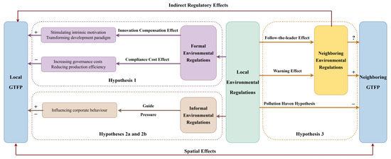
Figure 1.
Mechanism analysis diagram by Figdraw.
4. Research Design
4.1. Sample and Variables
This study included 284 prefectures and cities from the four main regions of China (East Coast, Central, West, and Northeast). These regions account for over 95% of the total 293 prefectures and cities in China. The study covers a period from 2003 to 2020, which guarantees the wide range and inclusiveness of the data. This enables thorough research on the developmental status of different regions in China, with substantial evidence. To ensure the consistency of the sample data, merged and newly established cities, such as Laiwu city in Shandong Province and Sansha city in Hainan Province, were excluded. The calculation data for each variable were obtained from the “China City Statistical Yearbook”, the “China Environmental Statistical Yearbook”, the National Intellectual Property Administration, government work reports of various cities, and the China Meteorological Data Network. A few missing data points were supplemented through linear interpolation.
4.2. Explanatory Variables
Urban green total factor productivity essentially aims to achieve urban economic growth with minimal environmental costs and inputs. Labor, capital, and energy serve as input variables, while GDP and pollutant emissions serve as output variables. Specifically, capital input refers to the studies by Zhang et al. [56] and Shan [57] to calculate the actual capital stock of each region using the formula . The formula assumes an initial capital stock of 10% of the initial fixed asset investment and uniformly sets the fixed asset depreciation rate at 9.6%. This allows for the calculation of each city’s capital stock using 2003 as the base period. Labor input is represented by the sum of the number of urban unit employees and the number of urban private and individual employees at the end of the period. Energy input is characterized by annual electricity consumption in urban areas [58]. Desired output is measured by calculating the real GDP of each city at constant prices in 2003. Undesired output is represented by a comprehensive index that includes industrial wastewater discharge, industrial sulfur dioxide emissions, industrial smoke (dust) emissions, etc. After being negatively transformed, the entropy weight method is used to combine them into an undesirable indicator. Based on the above, a super-efficiency SBM model [59,60], including undesired outputs, is constructed for measurement as follows:
In the aforementioned model, assuming there are decision-making units (DMUs) in the production system, each DMU is composed of three input–output vectors: input, desirable output, and undesirable output. These vectors can be expressed as: , , and . are matrices defined as follows: , , , .
Additionally, the objective function value represents the efficiency score of a DMU, which can exceed one. represents the k-th decision unit among decision units, which is the evaluated object. represents the number of inputs per decision unit. and represent the number of desirable and undesirable outputs. is a constant vector, representing the weights of the corresponding factors.
It should be noted that the above improved super-efficiency SBM model, which includes unexpected outputs, is carried out under the assumption of constant return to scale (CRS). In addition, the above model can also be extended to the variable rate of return on the scale (VRS) situation, which requires adding to the above model. Hence, this paper employs CRS as the setting for the aforementioned model, which is consistent with the setting of previous studies [61,62]. Meanwhile, to verify the accuracy of the conclusions, the robustness test uses VRS to recompute GTFP in the section that substitutes the explained variable.
4.3. Core Explanatory Variables
Previous studies suggest that most scholars tend to rely on a single statistical measure when evaluating formal environmental regulation (). Nevertheless, it is crucial to acknowledge that this indicator solely encompasses one aspect of formal environmental control and does not offer a holistic perspective. This article examines the proportion of environmental words in the government work report, expressed as a percentage of the total number [63,64]. The phrases encompass environmental protection, pollution, energy consumption, emission reduction, sewage, ecology, green, low carbon, air, chemical oxygen demand, sulfur dioxide, carbon dioxide, PM10, and PM2.5. The Chinese government work report functions as a strategic document that offers recommendations to organizations. This indicator can accurately assess the degree of attention and leadership demonstrated by local governments in the field of environmental protection. Released at the beginning of the year, this product remains unaffected by any external events that may occur later in the year, effectively minimizing any internal problems. In order to make the indicator comparable to informal environmental control, it is multiplied by 100 because the original data is of a modest scale.
This study investigates the impact of education level, income level, and population density on environmental protection behavior. The measure of informal environmental regulation () is used, as defined by Sheoli et al. [65]. These parameters are represented by using the number of students enrolled in general higher education schools, the average wage of employees, and the population density per square kilometer in each region as proxies. As individuals’ level of education increases, they are more inclined to come across knowledge on environmental conservation, fully grasp the importance of environmental issues, and actively participate in appropriate environmental protection efforts. The enrollment statistics of students in general higher education institutions serve as a more precise indicator of educational accomplishment and can offer valuable information about the educational norms in a particular area and the potential ability of its population to protect the environment. Moreover, those with higher income levels tend to have a stronger desire for better living standards and environmental conditions. They place a high value on ensuring their living environment is comfortable and safe, and they are prepared to spend money to improve the overall quality of the environment. Therefore, those living in areas with higher income levels are more likely to participate in efforts to protect the environment. Finally, environmental problems tend to attract more attention in areas of high population density, and at the same time, high population density means that more people can participate in environmental actions, creating a greater force for environmental protection. Therefore, this study uses the entropy weighting approach to generate the informal environmental regulation variable by standardizing the three variables.
4.4. Control Variables
The study’s control variables include the following:
Government intervention (GOV): This variable is measured by the ratio of general government budget expenditure to GDP during the same period. This indicator reflects the extent to which the government intervenes in the economy, which can have implications for environmental regulation and economic growth.
Degree of openness to the outside world (OPEN): This variable is assessed by the proportion of total imports and exports to GDP in the corresponding period. A higher degree of openness indicates greater integration with the global economy, which may affect environmental standards and policies due to international trade and investment flows.
Level of technological innovation (TEC): This variable is determined by the ratio of regional invention patent authorizations to national authorizations in the same year. Technological innovation is crucial for promoting green growth and reducing environmental impacts through more efficient and cleaner production methods.
Level of financial development (MAR): This variable is gauged by the ratio of the balance of loans from financial institutions at the end of the year to GDP during the same period. Financial development can facilitate access to capital for environmentally friendly investments and technologies, thus influencing the effectiveness of environmental regulation.
Including these control variables in the analysis helps to isolate the specific effects of formal and informal environmental regulations on urban GTFP by accounting for other potential influencing factors. In addition to these control variables, the analysis controls for year- and individual-fixed effects. The definitions of these control variables are provided in Table 1.

Table 1.
Definition of variables.
4.5. Econometric Model Construction
4.5.1. Two-Way Fixed Effects Model
Based on the theoretical analysis presented earlier, environmental regulation may have a non-linear impact on green total factor productivity [66]. Therefore, to depict the potential positive U-shaped effect of environmental regulation on GTFP, this article includes both the linear and quadratic terms of the environmental regulation variable in the two-way fixed effects model, as shown in Model (1). By including both terms, the model can capture the possibility that the relationship between environmental regulation and GTFP is not linear but may follow a curved pattern, specifically a “U” shape. This trend suggests that initially, an increase in environmental regulation may have a negative impact on GTFP, but as the level of regulation continues to increase, it eventually leads to a positive impact on GTFP. Including these terms in the regression model allows for a more nuanced understanding of the relationship between environmental regulation and GTFP, acknowledging its complexity and the potential for non-linear effects.
In Equation (1), is a constant term, while and are coefficients to be estimated. The variables and represent city and year, respectively. denotes the GTFP of city in year . represents the level of environmental regulation in city in year (where = 0 indicates formal environmental regulation and = 1 indicates informal environmental regulation). represents all the control variables. represents city-specific fixed effects, represents time-specific fixed effects, and is the random error term.
4.5.2. Spatial Panel Model
To analyze the spatial spillover effects of dual environmental regulation, we construct a spatial panel model.
First, drawing on the research of Bu et al. [67], we construct the following spatial weight matrices. The first type is the geographic distance matrix (), whose element represents the reciprocal of the spherical distance calculated from the latitudinal and longitudinal coordinates between city and city . The second type is the geoeconomic matrix (), which is constructed by multiplying the geographic distance matrix () with an economic matrix (). The elements of are represented by the logarithm of the absolute difference between the annual average per capita GDP of city and city .
Second, before constructing the spatial panel model, it is necessary to conduct a spatial autocorrelation test. In this paper, the global Moran’s I index is used to test the spatial correlation characteristics of the GTFP between regions. The calculation formula is , where represents 284 cities, is the spatial weight, and and are the GTFP and its city-level mean, respectively. The results are shown in Table 2. As shown in the table, regardless of whether the geographic distance matrix or the economic geographic matrix is used, Moran’s I is positive [68], and most of the corresponding p values are significant at the 1% level. This indicates that the GTFP at the city level in China is not randomly distributed but shows obvious positive spatial correlation and dependence characteristics, which is similar to the research results of Cheng et al. [69].
Table 2.
Global Moran index of China’s GTFP from 2003 to 2020.
Figure 2 shows scatter plots of the city-level GTFP distributions for four representative years, using the geographic distance matrix as an example. The scatter plots show a gradual dispersion toward the first and third quadrants over time, indicating a significant positive spatial spillover effect of GTFP. Therefore, the promotion of GTFP will create a virtuous cycle between regions, contributing to accelerating the achievement of sustainable economic development and improving the regional innovation environment.
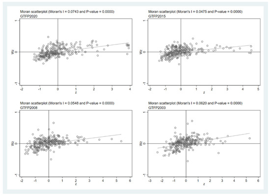
Figure 2.
Scatter plot of China’s city−level GTFP for several years under the geographical weight matrix.
Finally, we construct the following spatial econometric model:
In Equation (2), and are all parameters to be estimated. Among them, and measure the direct effects of environmental regulation and control variables on GTFP, respectively, while and measure their indirect effects.
5. Empirical Results and Analysis
5.1. Descriptive Statistics and Preliminary Testing
The descriptive statistics of the variables are shown in Table 3. As shown in the table, there are significant differences in the levels of GTFP across different cities in China at the current stage, and there are also large differences in other statistical indicators. For the initial testing, the variance inflation factor (VIF) was used to conduct a multicollinearity test. The results showed that the average VIF of the variables was less than five, indicating that there was no serious multicollinearity among the selected variables. Second, the Kao test and Pedroni test strongly rejected the null hypothesis of “no cointegration relationship” at the 1% level. Therefore, the panel data used in this paper can be considered cointegrated, and subsequent analysis can be carried out.
Table 3.
Descriptive statistics of the variables.
5.2. Regression Analysis of the Two-Way Fixed Effects Model
5.2.1. Baseline Regression Results
After conducting the Hausman test, the results showed a p value less than 0.01, rejecting the random effects assumption and opting for the fixed effects model. Furthermore, after including annual dummy variables in the model, the joint significance test also indicated a p value less than 0.01, rejecting the hypothesis of “no time effect”. Therefore, this study ultimately selected the two-way fixed effects model and employed cluster-robust standard errors to eliminate the impact of heteroscedasticity on the model, estimating at the city level.
Table 4 presents the regression analysis results. Specifically, the primary term’s coefficient for formal environmental regulation is significantly negative, while the quadratic term’s coefficient is significantly positive. This indicates that formal environmental regulation has a positive U-shaped impact on GTFP. In other words, lower levels of formal environmental regulation inhibit GTFP growth, with firms primarily exhibiting a “compliance cost effect”. However, as the intensity of formal environmental regulation continues to increase, its impact shifts from hindrance to promotion, and firms begin to demonstrate an “innovation compensation effect”. This discovery provides evidence in favor of Hypothesis 1, which posits that the impact of formal environmental regulation on GTFP exhibits a positive U-shaped pattern. Initially, there is a notable negative influence, which later transitions into a major positive effect.
Table 4.
Baseline regression results of dual environmental regulations on GTFP.
The primary term coefficient of informal environmental regulation is insignificant, but the quadratic term coefficient is significantly positive and much greater than the primary term. This finding suggests that the impact of informal environmental regulation on GTFP is non-linear. At lower levels, informal environmental regulation has a limited promotional effect on GTFP; however, as its intensity continues to increase due to the presence of network diffusion effects, its impact on GTFP exhibits a marginally increasing trend. This finding supports Hypothesis H2a, which suggests that informal environmental control has a non-linear effect on GTFP with a marginal incremental effect. Furthermore, this non-linear impact aligns with the research findings of Tian et al. [70], Wang et al. [71], and Zou et al. [72].
Calculations reveal that the inflection point for the change in the impact of formal environmental regulation is greater than the average level of formal environmental regulation in China. This implies that, on average, the current level of formal environmental regulation in various cities across China primarily manifests as a “compliance cost effect” on GTFP. Moreover, to assess the robustness of the results, Models (5) and (6) incorporate both formal and informal environmental regulations into the same model for estimation. The signs and significance of the coefficients remain unchanged, providing preliminary evidence of the robustness of the findings.
Additionally, referring to the research of Haans et al. [73], for formal environmental regulation, the quadratic term coefficient is significantly positive, with an inflection point of 0.825 falling within the range of [0, 1.239]. Specifically, when formal environmental regulation takes its minimum value of 0, the slope of the curve is −0.091, which is less than 0; when it takes its maximum value of 1.239, the slope of the curve is 0.046, which is greater than 0. Similarly, the inflection point for informal environmental regulation is 0.057, which is within its own range of [0.018, 0.845]. At its maximum value of 0.845, the slope is greater than 0. Therefore, it can be concluded that there exists a significant positive U-shaped relationship between dual environmental regulations and GTFP.
5.2.2. Robustness Testing and Endogeneity Issue Solving
To verify the reliability of the above conclusions, this paper adopts the following methods: First, the explained variable is replaced by modifying the assumption of constant returns to scale in the super-efficiency SBM model to variable returns to scale and recalculating GTFP. The results are shown in Model (7-1). Additionally, the explanatory variables are replaced with four individual indicators: the industrial sulfur dioxide removal rate, the industrial solid waste comprehensive utilization rate, the domestic sewage treatment rate, and the domestic waste harmless treatment rate. After positive transformation, the entropy weight method [74,75] is used to recalculate the formal environmental regulation level. The principal component analysis method [76] is applied to remeasure the original informal environmental regulation indicators, and the results are presented in Model (7-2).
Second, extreme values are deleted by performing a 1% winnowing on the original data to eliminate their impact on the study. The results are shown in Model (8). Third, interfering samples were excluded. Specifically, national central cities (Beijing, Shanghai, Guangzhou, Tianjin, Chongqing, Wuhan, Zhengzhou, Chengdu, and Xi’an) were removed from the analysis due to their relative advantages in geographical location, resource allocation, and other aspects. The regression results after exclusion are presented in Model (9).
Fourth, the sample period is adjusted by using data from 2005 to 2015 for regression (during this period, China’s GDP growth rate remained above 7% and exhibited an inverted U-shaped trend). The results are displayed in Model (10). Fifth, considering the possible lag effect of environmental regulation on GTFP, the explanatory variables are lagged by one period. The results are shown in Model (11).
Sixth, to address the issue of autocorrelation or clustering in the disturbance terms of different years within the same province, robust standard errors clustered at the province level are used for re-estimation. The results are presented in Model (12). Second, a Tobit regression model is constructed to account for the fact that GTFP comprises non-negative truncated data and is a limited dependent variable. A random effects Tobit panel model [77] is employed for regression, and bootstrap robust standard errors are used. The results indicate that both the LR and Wald regressions are significantly positive at the 1% level, as shown in Model (13).
Finally, the issue of endogeneity is addressed using the instrumental variable method. Specifically, annual precipitation data and lagged first-order and second-order terms of formal environmental regulation are selected as instrumental variables for estimating formal environmental regulation. For informal environmental regulation, annual temperature, the lagged first-order term of informal environmental regulation, and the lagged second-order term are chosen as instrumental variables. The parameter estimation results are shown in Model (14). The model tests reveal that there is no problem with weak instrumental variables and significantly reject the hypothesis of under-identification. Additionally, there is no issue with over-identification.
As shown in Table 5, the estimated coefficients of the first-order and second-order terms of formal environmental regulation, as well as the second-order term of informal environmental regulation, remain consistent in terms of sign and significance, with minor differences in coefficient magnitudes. However, they all satisfy the fact that the coefficient of the first-order term of formal environmental regulation is greater than that of the second-order term, and the coefficient of the second-order term of informal environmental regulation is greater than that of the first-order term. This finding aligns with the results of the benchmark regression model presented above, indicating that the analysis passes the robustness test and confirms the validity of Hypotheses 1 and 2a.
Table 5.
Robustness test results of the benchmark regression.
5.2.3. Heterogeneity Analysis
Drawing on the studies of Li et al. [78], Peng et al. [79], and Liu et al. [80], the following regional heterogeneity analysis was conducted. The results of the heterogeneity analysis presented in Table 6 indicate the following:
Table 6.
Results of heterogeneity analysis.
First, formal environmental regulations have a significant effect on the Yangtze River Delta and the Pearl River Basin, but not on the Bohai Rim Economic Circle. One possible explanation is that the Bohai Rim Economic Circle includes heavy industrial provinces in China, such as Hebei, Shandong, and Liaoning. On the one hand, although local governments have formally established policies for environmental regulation, “3-high” industries (those with high energy consumption, high pollution, and high emissions) tend to constitute the economic pillars of these cities, and GDP is still the main indicator for evaluating the performance of local governments at this stage. Therefore, in the process of policy implementation, environmental regulations often pose a conundrum to economic growth, resulting in a failure to form a substantial “compliance cost effect”. On the other hand, the proportion of traditional “3-high” industries in the local economy is too high, and overall, green transformation will face extremely high transformation costs and relative difficulties. Therefore, an “innovation compensation effect” has not yet been formed. This study suggests that these two factors led to the nonsignificant effect of formal environmental regulations on the GFTP in the Bohai Rim Economic Circle.
Second, the primary term for formal environmental regulations has a significant negative impact on the Silk Road Economic Belt, whereas the secondary term is positive but not significant. A possible reason is that the Silk Road Economic Belt mainly consists of cities in Northwest China with relatively simple industrial structures and a possibly high proportion of “3-high” industries. Therefore, once environmental regulations are implemented, these industries may be significantly affected, leading to a decrease in output value and thus a reduction in GTFP, manifesting as a strong “compliance cost effect”. The positive but insignificant secondary term may be because the implementation of formal environmental regulations in the Silk Road Economic Belt may not have brought about the expected environmental improvement effects, or the region may not have sufficient innovative elements to generate an “innovation compensation effect” to improve GTFP. Finally, formal environmental regulations have a significant effect on non-resource-based cities but not on resource-based cities, possibly because resource-based cities focus more on economic growth than on the implementation of environmental policies.
Informal environmental regulations are significantly positive in all regions except the Pearl River Basin. One possible explanation is that the industrial structure of the Pearl River Basin has a high proportion of environmentally friendly industries, such as services and high-tech industries, while the proportion of “3-high” industries that easily attract public attention is relatively low. As a result, local residents do not pay much attention to environmental pollution issues, leading to the nonsignificant, marginally increasing effect of informal environmental regulations in the region. In addition, judging from the secondary term coefficients, the marginally increasing effect of informal environmental regulations on GFTPs in resource-based cities is the strongest. This means that in resource-based cities, due to the high proportion of “3-high” industries in the city’s GDP, local residents pay more attention to pollution issues, and the network diffusion effect of informal regulations is stronger. Therefore, when the level of informal environmental regulation is below the threshold, despite the low level of regulation, this strong network diffusion effect is highly likely to cause online attention and public opinion, leading “3-high” enterprises to tend to take short-term measures such as shutting down production to respond to public opinion. Coupled with the high proportion of “3-high” industries in resource-based cities, shutting down production has a significant negative impact on the overall output of the city, thereby reducing GTFP. However, as the intensity of informal regulations crosses the threshold, fundamental changes in the social environment will occur, forcing enterprises to adopt green innovations to adapt to higher levels of environmental regulation, which in turn will have a more significant promoting effect on the GFTP. In summary, the results of the analyses in this section strongly support Hypothesis H2b that informal environmental regulation has a U-shaped effect in certain regions and cities, such as the Silk Road Economic Belt and resource cities, which means that informal environmental regulation initially has a negative effect on GTFP and then turns positive.
6. Regression Analysis of Spatial Panel Models
To construct an appropriate spatial panel model, the data on China’s urban GTFP and its influencing factors from 2003 to 2020 were subjected to Lagrange multiplier (LM), Wald, and likelihood ratio (LR) tests. As shown in Table 7, the LM test results indicate the presence of both spatial error and spatial lag effects in the model, suggesting the use of the SDM (spatial Durbin model). Both the Wald and LR tests reject the null hypothesis at the 1% significance level, indicating that the SDM does not degenerate into the SEM (spatial error model) or the SLM (spatial lag model). The Hausman test results indicate that a fixed effects model should be adopted. Further comparisons between urban fixed effects, temporal fixed effects, and double-fixed effects (both urban and temporal) revealed that an SDM model with urban–temporal double-fixed effects should be adopted.
Table 7.
Test results for spatial model selection.
The spatial Durbin model (SDM), compared to general regression models, incorporates a spatial weight matrix into its design, enabling it to capture not only local effects but also potential spillover effects to neighboring areas resulting from variable changes. However, the point estimates from the model alone may not adequately explain the spatial spillover effects across regions, necessitating the calculation of both direct and indirect explanatory variables. Therefore, drawing from the research of LeSage et al. [81] and Ge et al. [82], we decompose the SDM. The direct effects reflect the impact of dual environmental regulations on the GTFP of the city under consideration, while the indirect effects characterize the spatial spillover effects of these regulations on the GTFP of neighboring cities.
In Table 8, Models (21), (22), and (25) present estimation results based on the geographical distance matrix, while Models (23), (24), and (26) are based on the economic geography matrix. Specifically, models (21) and (23) focus on formal environmental regulation parameters, while models (22) and (24) concentrate on informal environmental regulation parameters. According to Panel A, regardless of whether the analysis is based on the geographical distance matrix or the economic geography matrix, the spatial autoregressive coefficient rho is significantly positive. This indicates that an improvement in the GTFP of a local city promotes the GTFP of neighboring cities, exhibiting a notable positive spillover effect [2], which aligns with previous findings from Moran’s index studies.
Table 8.
Spatial effects and decomposition of dual environmental regulations on GTFP.
In terms of the direct effects of environmental regulations on GTFP, the primary term for formal environmental regulation is significantly negative, while the quadratic term is significantly positive. For informal environmental regulation, the primary term is not significant, but the quadratic term is significantly positive. These results align with the baseline regression outcomes, further reinforcing that Hypotheses 1 and 2a remain valid even after considering possible spatial influences. In regard to indirect effects, both formal and informal environmental regulations have negative primary term coefficients, suggesting that they have a suppressive influence on the GTFP development of neighboring cities. This indicates a tendency for firms to shift pollution to neighboring areas under the pressure of dual environmental regulations, exhibiting a “pollution haven effect”. The positive quadratic term coefficients suggest that as the level of dual environmental regulation increases in a given region, it can synergistically promote the GTFP growth of neighboring cities.
Considering the impact of dual environmental regulations on local GTFP, we posit that as the level of these regulations gradually rises in a region, locally polluting firms, pressured by the government and public opinion, may relocate to neighboring cities with lower regulatory standards, thereby inhibiting the growth of GTFP in those areas. However, during this process, neighboring cities’ governments and informal environmental forces may gradually strengthen their own regulations through exposure and learning, leading to a “follow-the-leader” or “warning effect” that ultimately drives an increase in their gross total growth factor. Based on the above comprehensive analysis, it can be concluded that Hypothesis 3 is supported. The study reveals that the influence of dual environmental regulation on GTFP in neighboring cities exhibits a positive U-shaped pattern, initially reducing and then increasing.
Additionally, the SDM estimations based on both types of spatial weight matrices show consistent results in terms of coefficient signs and significance levels. Furthermore, Panel B, which incorporates both formal and informal environmental regulations into the model simultaneously, yields results that align with the previous analysis. Therefore, we can consider the findings to have passed the robustness test.
7. Conclusions and Recommendations
7.1. Conclusions
This study focused on 284 cities in China from 2003 to 2020 and precisely identified the relationship between dual environmental regulation and GTFP through the construction of a two-way fixed effects model. Simultaneously, the SDM was introduced to investigate the specific impact of local environmental regulation on the GTFP of neighboring cities. The research findings are as follows:
First, from an overall trend perspective, the impact of dual environmental regulation on local GTFP exhibits a positive U-shaped trend, which is consistent with the findings of Tian et al. [70]. This conclusion remains valid after we replace the explanatory variables, delete extreme values, eliminate interfering samples, adjust the sample period, lag the explanatory variables by one period, replace robust standard errors, adopt Tobit regression, discuss endogeneity issues, and introduce spatial panel models. Specifically, when formal environmental regulation is low, it inhibits the improvement of GTFP, and enterprises exhibit a “compliance cost effect”. As its intensity continues to increase, it gradually shifts from inhibition to promotion, and enterprises demonstrate an “innovation compensation effect”. The impact of informal environmental regulation on GTFP is characterized by non-linear features and exhibits a “marginal increasing effect”, which differs from previous research findings.
Second, in the analysis of heterogeneity, formal environmental regulation plays a significant role in the Yangtze River Delta, the Pearl River Basin, and non-resource-based cities. However, this may not have had a significant effect on the Bohai Rim Economic Circle or resource-based cities, possibly due to the prioritization of economic growth over environmental regulation in these regions. Informal environmental regulation is significantly positive in all regions except the Pearl River Basin, and this effect is more pronounced in resource-based cities. A possible reason is that enterprises in the Pearl River Basin are strongly aware of ecological environmental protection, and the proportion of “3-high” industries in the industrial structure is relatively low. In contrast, resource-based cities are more dependent on the output value created by “3-high” enterprises.
Finally, in the spatial panel model, whether under the geographical distance matrix or the economic geography matrix, the SDM estimation results show that an increase in GTFP in local cities promotes GTFP in neighboring cities. However, the effect of dual environmental regulation on the GTFP of neighboring cities is initially inhibitory and then promotional, exhibiting a “pollution haven hypothesis” followed by a “follow-the-leader effect” or “warning effect”. The direction of the impact of formal environmental regulation on local and neighboring areas is consistent, exhibiting a positive U-shaped trend. The conclusion holds in two different matrices and in the SDM model that simultaneously incorporates dual environmental regulation, demonstrating the robustness of the spatial panel model results.
7.2. Recommendations
Based on the above findings, this paper proposes the following recommendations to accelerate the improvement of GTFP levels in various cities, formulate more effective environmental policies, and further establish a long-term mechanism for green development among regions.
First, the concept of green development should be adopted, and environmental regulation should be continuously strengthened. Although formal environmental regulation at the government level may have a certain negative impact on urban GTFP in the initial stage, local governments must unwaveringly uphold the concept of green development, continuously strengthen the intensity of environmental regulation, and improve related policies, regulations, and systems to completely change the policy environment and expectations of enterprise operations. This approach will help to overcome the “environmental regulation trap” and achieve a reversal of the impact on GTFP. For informal environmental regulation, we need to attach importance to its “marginal increasing effect” on GTFP, fully leverage the power of the people, effectively use social networks as a “multiplier” for environmental regulation effects, correctly guide online public opinion, create a social atmosphere that advocates green development, and continuously promote economic green growth.
Second, it is important to accurately perceive regional differences in the effects of environmental regulation, adopt measures to address local conditions, and implement classified policies. For example, in resource-based cities, formal environmental regulation may not have a significant effect on promoting GTFP due to the relatively greater difficulty of the green economic transformation. However, it remains crucial to actively consider the role of these cities, foster a synergistic relationship between industrial and environmental policies, and strive for a coordinated development of the resource environment, the economy, and society in resource-based cities, even if it means sacrificing time for effectiveness. In terms of informal regulation, it is necessary to guide enterprises to correctly treat public supervision and demands, reduce negative response measures, encourage them to embark on the path of green development early, and avoid falling into the “environmental regulation trap”.
Third, cooperation and communication between regional and local governments should be strengthened. In all aspects, local governments should strengthen cooperation and communication, share environmental governance experiences and technologies, and jointly address environmental and development issues. Governments can promote regional cooperation mechanisms among cities, establish green innovation platforms, and facilitate resource sharing. Moreover, neighboring local governments can learn from each other’s policies, strengthen collaboration, and minimize the “pollution haven effect” to fully leverage the positive spatial spillover effect of GTFP growth and promote green transformation and development throughout the region.
In addition, we highlight the limitations of the current research and potential future research directions: (1) This research specifically examines Chinese cities. Although China serves as a representative example of an emerging economy, additional evidence is necessary to ascertain the applicability of this paper’s findings to other emerging economies, including India, Brazil, and others. (2) This study’s analysis suggests that informal environmental regulations have a marginally increasing effect on GTFP, and a series of tests support this conclusion. However, according to the fundamental principles of economics, the phenomenon of marginally increasing effects typically exists within a specific range. The scope of the data samples available for analysis limits the conclusions drawn in this study. Further data support is required to determine the extent to which informal environmental regulations generate marginally increasing effects on GTFP.
Author Contributions
Conceptualization Z.Z.; data organization, F.Z.; formal analysis, Z.Z.; funding acquisition, Y.Z.; surveys, Z.Z.; methodology, Z.Z.; project management, Y.Z.; resources, Z.Z.; software, Z.Z.; supervision, Y.Z.; validation, Z.Z.; visualization, F.Z.; writing—original drafts, Z.Z.; writing—review and editing, F.Z. All authors have read and agreed to the published version of the manuscript.
Funding
This research received no external funding.
Institutional Review Board Statement
Not applicable.
Informed Consent Statement
Not applicable.
Data Availability Statement
The datasets used or analyzed during the current study are available from the yearbooks or the corresponding author upon reasonable request.
Conflicts of Interest
The authors declare that they have no conflicts of interest.
References
- Sun, Y.P.; Asif, R.; Renatas, K.; Bao, Q. High-speed rail and urban green productivity: The mediating role of climatic conditions in China. Technol. Forecast. Soc. Chang. 2022, 185, 122055. [Google Scholar] [CrossRef]
- Zhao, X.; Nakonieczny, J.; Jabeen, F.; Shahzad, U.; Jia, W. Does green innovation induce green total factor productivity? Novel findings from Chinese city level data. Technol. Forecast. Soc. Chang. 2022, 185, 122021. [Google Scholar] [CrossRef]
- Zhang, H.P.; Dong, Y. Measurement and spatial correlations of green total factor productivities of Chinese provinces. Sustainability 2022, 14, 5071. [Google Scholar] [CrossRef]
- Kathuria, V. Informal regulation of pollution in a developing country: Evidence from India. Ecol. Econ. 2006, 63, 403–417. [Google Scholar] [CrossRef]
- Zhou, Q.; Zhong, S.H.; Shi, T.; Zhang, X.L. Environmental regulation and haze pollution: Neighbor-companion or neighbor-beggar? Energy Policy 2021, 151, 112183. [Google Scholar] [CrossRef]
- Huang, X.L.; Tian, P. How does heterogeneous environmental regulation affect net carbon emissions: Spatial and threshold analysis for China. J. Environ. Manag. 2023, 330, 117161. [Google Scholar] [CrossRef]
- Cui, B.Q.; Shui, Z.H.; Yang, S.; Lei, T.Y. Evolutionary game analysis of green technology innovation under the carbon emission trading mechanism. Front. Environ. Sci. 2022, 10, 997724. [Google Scholar] [CrossRef]
- Liu, Y.Q.; Zhu, J.L.; Li, E.Y.; Meng, Z.Y.; Song, Y. Environmental regulation, green technological innovation, and eco-efficiency: The case of Yangtze river economic belt in China. Technol. Forecast. Soc. 2020, 155, 119993. [Google Scholar] [CrossRef]
- Cole, M.A.; Elliott, R.J.R.; Shimamoto, K. Industrial characteristics, environmental regulations and air pollution: An analysis of the UK manufacturing sector. J. Environ. Econ. Manag. 2004, 50, 121–143. [Google Scholar] [CrossRef]
- Zhou, M.; Govindan, K.; Xie, X.B.; Yan, L. How to drive green innovation in China’s mining enterprises? Under the perspective of environmental legitimacy and green absorptive capacity. Resour. Policy 2021, 72, 102038. [Google Scholar] [CrossRef]
- Ouyang, X.; Shao, Q.L.; Zhu, X.; He, Q.Y.; Xiang, C.; Wei, G.E. Environmental regulation, economic growth and air pollution: Panel threshold analysis for OECD countries. Sci. Total. Environ. 2019, 657, 234–241. [Google Scholar] [CrossRef] [PubMed]
- Bu, C.Q.; Zhang, K.X.; Shi, D.Q.; Wang, S.Y. Does environmental information disclosure improve energy efficiency? Energy Policy 2022, 164, 112919. [Google Scholar] [CrossRef]
- Wang, W.D.; Li, Y.Y.; Lu, N.; Wang, D.; Jiang, H.L.; Zhang, C.J. Does increasing carbon emissions lead to accelerated eco-innovation? Empirical evidence from China. J. Clean. Prod. 2020, 251, 119690. [Google Scholar] [CrossRef]
- Qian, X.Y.; Wang, D.; Wang, J.; Chen, S. Resource curse, environmental regulation and transformation of coal-mining cities in China. Resour. Policy 2019, 74, 101447. [Google Scholar] [CrossRef]
- Wang, Z.H.; Wang, N.; Hu, X.Q.; Wang, H.P. Threshold effects of environmental regulation types on green investment by heavily polluting enterprises. Environ. Sci. Eur. 2022, 34, 26. [Google Scholar] [CrossRef]
- Wang, T.; Peng, J.C.; Lei, W. Heterogeneous effects of environmental regulation on air pollution: Evidence from China’s prefecture-level cities. Environ. Sci. Pollut. Res. 2021, 28, 25782–25797. [Google Scholar] [CrossRef] [PubMed]
- Goldar, B.; Banerjee, N. Impact of informal regulation of pollution on water quality in rivers in India. J. Environ. Manag. 2004, 73, 117–130. [Google Scholar] [CrossRef]
- Langpap, C.; Shimshack, P.J. Private citizen suits and public enforcement: Substitutes or complements? J. Environ. Econ. Manag. 2010, 59, 235–249. [Google Scholar] [CrossRef]
- Song, M.L.; Du, J.T.; Tan, K.H. Impact of fiscal decentralization on green total factor productivity. Int. J. Prod. Econ. 2018, 205, 359–367. [Google Scholar] [CrossRef]
- Ibrahim, R.L.; Ajide, K.B.; Usman, M.; Kousar, R. Heterogeneous effects of renewable energy and structural change on environmental pollution in Africa: Do natural resources and environmental technologies reduce pressure on the environment? Renew. Energ. 2022, 200, 244–256. [Google Scholar] [CrossRef]
- Pata, U.K.; Aydin, M.; Haouas, I. Are natural resources abundance and human development a solution for environmental pressure? Evidence from top ten countries with the largest ecological footprint. Resour. Policy 2021, 70, 101923. [Google Scholar] [CrossRef]
- Cheng, Z.H.; Kong, S.Y. The effect of environmental regulation on green total-factor productivity in China’s industry. Environ. Impact Assess. Rev. 2022, 94, 106757. [Google Scholar] [CrossRef]
- Li, K.; Lin, B.Q. Economic growth model, structural transformation, and green productivity in China. Appl. Energy 2017, 187, 489–500. [Google Scholar] [CrossRef]
- Xia, F.; Xu, J.T. Green total factor productivity: A re-examination of quality of growth for provinces in China. China Econ. Rev. 2020, 62, 101454. [Google Scholar] [CrossRef]
- Shen, W.F.; Zhang, D.Q.; Liu, W.B.; Yang, G.L. Increasing discrimination of DEA evaluation by utilizing distances to anti-efficient frontiers. Comput. Open. Res. 2016, 75, 163–173. [Google Scholar] [CrossRef]
- Jiang, Y.F.; Wang, H.Y.; Liu, Z.K. The impact of the free trade zone on green total factor productivity-evidence from the shanghai pilot free trade zone. Energy Policy 2021, 148, 112000. [Google Scholar] [CrossRef]
- Ren, W.H.; Ji, J.Y. How do environmental regulation and technological innovation affect the sustainable development of marine economy: New evidence from China’s coastal provinces and cities. Mar. Policy 2021, 128, 104468. [Google Scholar] [CrossRef]
- Yang, X.D.; Wang, W.L.; Wu, H.T.; Wang, J.L.; Ran, Q.Y.; Ren, S.Y. The impact of the new energy demonstration city policy on the green total factor productivity of resource-based cities: Empirical evidence from a quasi-natural experiment in China. J. Environ. Plann. Man. 2021, 66, 293–326. [Google Scholar] [CrossRef]
- Yang, Y.D. Can environmental regulations and R&D subsidies promote GTFP in pharmaceutical industry? Evidence from Chinese provincial panel data. Front. Public Health 2022, 10, 1018968. [Google Scholar] [CrossRef]
- Wang, Y.F.; Xie, L.; Zhang, Y.; Wang, C.Y.; Yu, K. Does FDI Promote or Inhibit the High-Quality Development of Agriculture in China? An Agricultural GTFP Perspective. Sustainability 2019, 11, 4620. [Google Scholar] [CrossRef]
- Sun, Y.X.; Zhang, M.Y.; Zhu, Y.C. Do Foreign Direct Investment Inflows in the Producer Service Sector Promote Green Total Factor Productivity? Evidence from China. Sustainability 2023, 15, 10904. [Google Scholar] [CrossRef]
- Lanoie, P.; Patry, M.; Lajeunesse, R. Environmental regulation and productivity: Testing the porter hypothesis. J. Prod. Anal. 2008, 30, 121–128. [Google Scholar] [CrossRef]
- Sun, X.L.; Zhang, R.; Yu, Z.F.; Zhu, S.C.; Qie, X.T.; Wu, J.X.; Li, P.P. Revisiting the porter hypothesis within the economy-environment-health framework: Empirical analysis from a multidimensional perspective. J. Environ. Manag. 2023, 349, 119557. [Google Scholar] [CrossRef] [PubMed]
- Ding, X.G.; Andrea, A.; Mohsin, S. Environmental administrative penalty, corporate environmental disclosures and the cost of debt. J. Clean. Prod. 2022, 332, 129919. [Google Scholar] [CrossRef]
- Wang, Y.; Dong, Y.; Sun, X.H. Can environmental regulations facilitate total-factor efficiencies in OECD countries? Energy-saving target VS emission-reduction target. Int. J. Green Energy 2023, 20, 1488–1500. [Google Scholar] [CrossRef]
- Zhang, H.M.; Zhu, Z.S.; Fan, Y.J. The impact of environmental regulation on the coordinated development of environment and economy in China. Nat. Hazards 2018, 91, 473–489. [Google Scholar] [CrossRef]
- Liu, J.H.; Wang, H.Y.; Ho, H.W.W.; Huang, L.C. Impact of heterogeneous environmental regulation on manufacturing sector green transformation and sustainability. Front. Environ. Sci. 2022, 10, 938509. [Google Scholar] [CrossRef]
- Gao, W.; Cheng, J.; Zhang, J. The influence of heterogeneous environmental regulation on the green development of the mining industry: Empirical analysis based on the system GMM and dynamic panel data model. Chin. J. Popul. Resour. Environ. 2019, 17, 154–175. [Google Scholar] [CrossRef]
- Wu, B.; Fang, H.Q.; Gady, J.; Li, G.L.; Wu, Z.Y. Environmental regulations and innovation for sustainability? Moderating effect of political connections. Emerg. Mark. Rev. 2022, 50, 100835. [Google Scholar] [CrossRef]
- Chen, L.; Li, W.L.; Yuan, K.B.; Zhang, X.Q. Can informal environmental regulation promote industrial structure upgrading? Evidence from China. Appl. Econ. 2022, 54, 2161–2180. [Google Scholar] [CrossRef]
- Guo, L.Y.; Hu, C.; Fan, M.J.; Mao, J.H.; Tian, M.; Wang, Z.H.; Wei, Y.Y. Does informal environmental regulation matter? Evidence on the different impacts of communities and ENGOs on heavy-polluting firms’ green technology innovation. J. Environ. Plan. Manag. 2023, 1–27. [Google Scholar] [CrossRef]
- Zheng, Q.Q.; Wan, L.; Wang, S.Y.; Chen, Z.X.; Li, J.; Wu, J.; Song, M.L. Will informal environmental regulation induce residents to form a green lifestyle? Evidence from China. Energy Econ. 2023, 125, 106835. [Google Scholar] [CrossRef]
- Peng, M.R.; Peng, S.C.; Jin, Y.L.; Wang, S.J. Government environmental information disclosure and corporate carbon performance. Front. Environ. Sci. 2023, 11, 1204970. [Google Scholar] [CrossRef]
- Shi, X.H.; Chen, X.; Han, L.; Zhou, Z.J. The mechanism and test of the impact of environmental regulation and technological innovation on high quality development. J. Comb. Optim. 2023, 45, 52. [Google Scholar] [CrossRef]
- Meyer, M.S.; Konisky, M.D. Adopting local environmental institutions: Environmental need and economic constraints. Political Res. Q. 2007, 60, 3–16. [Google Scholar] [CrossRef]
- Li, X.Z.; Wang, L.J.; Du, K.R. How do environmental regulations influence resource misallocation in China? The role of investment flows. Bus. Strategy Environ. 2023, 32, 538–550. [Google Scholar] [CrossRef]
- Song, M.L.; Zhao, X.; Shang, Y.P.; Chen, B.Y. Realization of green transition based on the anti-driving mechanism: An analysis of environmental regulation from the perspective of resource dependence in China. Sci. Total. Environ. 2019, 698, 134317. [Google Scholar] [CrossRef] [PubMed]
- Shen, J.; Wei, Y.D.; Yang, Z. The impact of environmental regulations on the location of pollution-intensive industries in China. J. Clean. Prod. 2017, 148, 785–794. [Google Scholar] [CrossRef]
- Zhang, C.; Tao, R.; Yue, Z.H.; Su, F.B. Regional competition, rural pollution haven and environmental injustice in China. Ecol. Econ. 2023, 204, 107669. [Google Scholar] [CrossRef]
- Li, M.J.; Du, W.J.; Tang, S.L. Assessing the impact of environmental regulation and environmental co-governance on pollution transfer: Micro-evidence from China. Environ. Impact Assess. Rev. 2021, 86, 106467. [Google Scholar] [CrossRef]
- Fredriksson, G.P.; Millimet, L.D. Strategic interaction and the determination of environmental policy across U.S. States. J. Urban Econ. 2002, 51, 101–122. [Google Scholar] [CrossRef]
- Konisky, M.D. Regulatory competition and environmental enforcement: Is there a race to the bottom? Am. J. Political Sci. 2007, 51, 853–872. [Google Scholar] [CrossRef]
- Zhong, S.; Li, J.; Zhao, R.L. Does environmental information disclosure promote sulfur dioxide (SO2) remove? new evidence from 113 cities in China. J. Clean. Prod. 2021, 299, 126906. [Google Scholar] [CrossRef]
- Centola, D. The spread of behavior in an online social network experiment. Science 2010, 329, 1194–1197. [Google Scholar] [CrossRef] [PubMed]
- Yu, X.; Zeng, Z.T. Impact of heterogeneous environmental regulation on total factor productivity: An empirical study based on China’s provincial data. Environ. Dev. Sustain. 2023, 1–23. [Google Scholar] [CrossRef]
- Zhang, J.; Wu, G.Y.; Zhang, J.P. Estimation of interprovincial material capital stock in China: 1952–2000. Econ. Res. 2004, 10, 35–44. [Google Scholar]
- Shan, H.J. Re-estimate of China capital stock K: 1952–2006. J. Quant. Tech. Econ. 2008, 25, 17–31. [Google Scholar]
- Gu, B.M.; Liu, J.G.; Ji, Q. The effect of social sphere digitalization on green total factor productivity in China: Evidence from a dynamic spatial Durbin model. J. Environ. Manag. 2022, 320, 115946. [Google Scholar] [CrossRef]
- Li, H.; Fang, K.N.; Yang, W.; Wang, D.; Hong, X.X. Regional environmental efficiency evaluation in China: Analysis based on the Super-SBM model with undesirable outputs. Math. Comput. Model. 2013, 58, 1018–1031. [Google Scholar] [CrossRef]
- Guo, R.; Yuan, Y.J. Different types of environmental regulations and heterogeneous influence on energy efficiency in the industrial sector: Evidence from Chinese provincial data. Energy Policy 2020, 145, 111747. [Google Scholar] [CrossRef]
- Yang, J.; Liu, X.J.; Ying, L.M.; Chen, X.D.; Li, M.H. Correlation analysis of environmental treatment, sewage treatment and water supply efficiency in China. Sci. Total Environ. 2020, 708, 135128. [Google Scholar] [CrossRef] [PubMed]
- Guan, X.Y.; Zhu, X.N.; Liu, X.J. Carbon Emission, air and water pollution in coastal China: Financial and trade effects with application of CRS-SBM-DEA model. Alex. Eng. J. 2022, 61, 1469–1478. [Google Scholar] [CrossRef]
- Zhao, S.L.; Teng, L.J.; Ekow, V.A.; Hu, H. Impacts of digital government on regional eco-innovation: Moderating role of dual environmental regulations. Technol. Forecast. Soc. Change 2023, 196, 122842. [Google Scholar] [CrossRef]
- Chen, Z.; Kahn, E.M.; Liu, Y.; Wang, Z. The consequences of spatially differentiated water pollution regulation in China. J. Environ. Econ. Manag. 2018, 88, 468–485. [Google Scholar] [CrossRef]
- Sheoli, P.; David, W. Informal regulation of industrial pollution in developing countries: Evidence from Indonesia. J. Polit. Econ. 1996, 104, 1314–1327. [Google Scholar] [CrossRef]
- He, Q.; Han, Y.W.; Wang, L. The impact of environmental regulation on green total factor productivity: An empirical analysis. PLoS ONE 2021, 16, e0259356. [Google Scholar] [CrossRef]
- Bu, Y.; Wang, E.D.; Qiu, Y.Y.; Möst, D. Impact assessment of population migration on energy consumption and carbon emis-sions in China: A spatial econometric investigation. Environ. Impact Assess. Rev. 2022, 93, 106744. [Google Scholar] [CrossRef]
- Wang, H.R.; Cui, H.R.; Zhao, Q.Z. Effect of green technology innovation on green total factor productivity in China: Evidence from spatial durbin model analysis. J. Clean. Prod. 2020, 288, 125624. [Google Scholar] [CrossRef]
- Cheng, Z.H.; Jin, W. Agglomeration economy and the growth of green total-factor productivity in Chinese Industry. Socio-Econ. Plan. Sci. 2022, 83, 101003. [Google Scholar] [CrossRef]
- Tian, Y.; Feng, C. The internal-structural effects of different types of environmental regulations on China’s green total-factor productivity. Energy Econ. 2022, 113, 106246. [Google Scholar] [CrossRef]
- Wang, X.L.; Shao, Q.L. Non-linear effects of heterogeneous environmental regulations on green growth in G20 countries: Evidence from panel threshold regression. Sci. Total. Environ. 2019, 660, 1346–1354. [Google Scholar] [CrossRef] [PubMed]
- Zou, H.; Zhang, Y.J. Does environmental regulatory system drive the green development of China’s pollution-intensive industries? J. Clean. Prod. 2022, 330, 129832. [Google Scholar] [CrossRef]
- Haans, R.F.; Pieters, C.; He, Z.L. Thinking about U: Theorizing and testing U- and inverted U-shaped relationships in strategy research. Strateg. Manag. J. 2016, 37, 1177–1195. [Google Scholar] [CrossRef]
- Zhang, M.L.; Li, B.Z. How to improve regional innovation quality from the perspective of green development? findings from entropy weight method and fuzzy-set qualitative comparative analysis. IEEE Access 2020, 8, 32575–32586. [Google Scholar] [CrossRef]
- Zhai, X.Q.; An, Y.F.; Shi, X.P.; Liu, X. Measurement of green transition and its driving factors: Evidence from China. J. Clean. Prod. 2022, 335, 130292. [Google Scholar] [CrossRef]
- Zhang, L.; Adom, P.K.; An, Y. Regulation-induced structural break and the long-run drivers of industrial pollution intensity in China. J. Clean. Prod. 2018, 198, 121–132. [Google Scholar] [CrossRef]
- Song, Y.; Yeung, G.; Zhu, D.L.; Xu, Y.; Zhang, L.X. Efficiency of urban land use in China’s resource-based cities, 2000–2018. Land Use Policy 2022, 115, 106009. [Google Scholar] [CrossRef]
- Li, B.; Wu, S.S. Effects of local and civil environmental regulation on green total factor productivity in China: A spatial Durbin econometric analysis. J. Clean. Prod. 2017, 153, 342–353. [Google Scholar] [CrossRef]
- Peng, Y.X.; Lin, H.Y.; Lee, J. Analyzing the mechanism of spatial–temporal change of green total factor productivity in Yangtze Delta Region of China. Environ. Dev. Sustain. 2022, 25, 14261–14282. [Google Scholar] [CrossRef]
- Liu, X.H.; Yang, J.J.; Xu, C.Z.; Li, X.C.; Zhu, Q.Y. Environmental regulation efficiency analysis by considering regional heterogeneity. Resour. Policy 2023, 83, 103735. [Google Scholar] [CrossRef]
- LeSage, P.J.; Pace, K.R. The biggest myth in spatial econometrics. Econometrics 2014, 2, 217–249. [Google Scholar] [CrossRef]
- Ge, T.; Hao, X.L.; Li, J.Y. Effects of public participation on environmental governance in China: A spatial durbin econometric analysis. J. Clean. Prod. 2021, 321, 129042. [Google Scholar] [CrossRef]

Disclaimer/Publisher’s Note: The statements, opinions and data contained in all publications are solely those of the individual author(s) and contributor(s) and not of MDPI and/or the editor(s). MDPI and/or the editor(s) disclaim responsibility for any injury to people or property resulting from any ideas, methods, instructions or products referred to in the content. |
© 2024 by the authors. Licensee MDPI, Basel, Switzerland. This article is an open access article distributed under the terms and conditions of the Creative Commons Attribution (CC BY) license (https://creativecommons.org/licenses/by/4.0/).