Abstract
The seriousness of vessel air pollution has forced the International Maritime Organization (IMO) to introduce a series of relevant laws and regulations. This paper proposes a monitoring scheme based on the synergistic operation of motherships and UAVs. This scheme innovatively adopts a harbor sea patrol vessel or the other official vessel (mothership) as the mobile power supply base for UAVs and realizes efficient and accurate monitoring of vessel air pollution in the pre-monitored area at sea by carrying multiple UAVs. The focus of this paper is on the path optimization problem for multi-UAV collaboration with mothership (MUCWM) monitoring, where the objective is to minimize the total monitoring time for MUCWM. The following three main aspects are studied in this paper: (1) multi-UAV monitoring path optimization; (2) the collaboration mechanism between the mothership and multiple UAVs; and (3) mothership traveling path optimization. In order to effectively solve the above problems, this thesis constructs a path optimization model for multi-UAV collaborative mothership monitoring of air pollution from vessels in port waters; solves the model using the improved adaptive differential evolution (IADE) algorithm; and verifies the effectiveness of the model and the algorithm by using the position data in the Automatic Identification System (AIS) of vessels in Ningbo Zhoushan Port. Through the performance comparison and sensitivity analysis of the algorithm, it is confirmed that the algorithm can effectively solve the path planning problem of the collaborative operation between the mothership and multiple UAVs. The research results in this paper not only help to reduce the air pollution level of harbor vessels and improve the efficiency of sea cruising but also play an important supporting role in the enforcement of relevant emission regulations.
1. Introduction
In recent years, international shipping has rapidly expanded as a low-cost way to transport bulk commodities [1], accounting for over 90% of global trade [2]. According to the United Nations’ 2023 Review of Maritime Transport report, maritime trade is expected to grow by 2.4% in the post-pandemic era [3]. However, as the shipping industry flourishes, the environmental issues associated with marine fuels are becoming more apparent [1]. Vessel air pollution is now recognized as the third primary source of pollution, after vehicle exhaust and industrial emissions. [4]. Vessels emit significant pollutants such as carbon dioxide (CO2), nitrogen oxides (NOX), sulfur oxides (SOX), and particulate matter (PM) while navigating. Global data indicate that SOX emissions from vessels make up 10–15% of total human activity emissions [5]. These pollutants not only lead to ocean acidification [1,6] but also cause various respiratory diseases in humans. Studies show that vessel pollution has become a major source of air pollution in port cities, particularly from container vessels powered by high-sulfur fuels exceeding 3.50% sulfur content, which severely pollute nearby waters and air [7].
Serious environmental and health concerns have compelled the International Maritime Organization (IMO) to take decisive actions. Since 2015, the IMO has established four Emission Control Areas (ECAs) in the Baltic Sea, the North Sea, North America, and the U.S. Caribbean. The organization intends to establish additional Emission Control Areas (ECAs) in various regions to minimize pollution from vessels [8]. The International Maritime Organization (IMO) now mandates that vessels entering these ECAs utilize fuel containing less than 0.1% m/m sulfur content [9]. In 2020, the IMO’s Marine Environment Protection Committee (MEPC) set a global limit on sulfur content in marine fuels at 0.50% m/m [10]. In the same year, the Maritime Safety Administration under China’s Ministry of Transportation declared the “2020 Global Marine Fuel Sulfur Restriction Implementation Plan” along with the “Guidelines for the Supervision and Management of Air Pollutant Emissions from Ships”. According to these guidelines, the sulfur content of fuel used by vessels in inland waterway emission control areas must be no more than 0.1% m/m. Additionally, the sulfur content in the fuel used by ships operating within coastal air pollution control areas and on international journeys in non-emission control areas should not surpass 0.5% m/m [11]. Despite these regulations, the extra costs of purchasing gas purification devices or using low-sulfur fuels lead some shipping companies to violate these rules to cut costs. Methods include using cheaper, high-sulfur fuels, shutting down pollution control equipment in ECAs, and falsifying vessel logs and fuel consumption records [1]. Historical data indicate that non-compliance rates can reach as high as 12.3% [11].
There are two main traditional methods for monitoring air pollution from vessels. The first is manual boarding, which includes taking oil samples, checking oil change records in the logbook, and using a rapid sulfur detector for marine fuel oil. The second method involves real-time tracking of air quality using land-based environmental monitoring stations. However, both methods have drawbacks. They are inefficient, susceptible to environmental influences, and offer limited monitoring coverage. This is particularly problematic during emergencies such as epidemics, when manual boarding and testing become almost impossible.
UAVs are characterized by high flexibility, no geographical restrictions, and high operability [12]. As UAV technology continues to develop, its use in the shipping industry is becoming increasingly widespread. UAVs are now used for port infrastructure security inspections, maritime oil spill monitoring, ship piloting, maritime smuggling detection, and hazardous chemical inspections at ports [13,14,15,16,17]. Additionally, UAVs have started to be employed in vessel air pollution monitoring. For instance, on 20 May 2020, a DJI M210 UAV, named “Rhinoceros V2” and equipped with a system for detecting air pollution, carried out exhaust gas measurements close to the Ganjiang Marine Office of the Yangzhou Maritime Bureau in China [18]. On 5 January 2021, Zhangjiagang Maritime Bureau used a UAV-mounted gas detector to detect a vessel with excessive sulfur emissions [19]; on 26 June 2022, Changshu Maritime Bureau used a UAV to monitor air pollution from vessels and inspected and found a vessel with an exhaust sulfur value of 3.0% m/m or more [20]; on 20 October 2022, the Port of Rotterdam Authority attempted to apply the new Aera3 UAV for monitoring air pollution emissions from vessels [21]. These instances show that UAVs are a feasible and promising tool for monitoring air pollution from vessels [7].
However, the above-mentioned studies are still nascent, with several critical issues needing resolution:
- (1)
- The energy constraints of UAVs [22].
- (2)
- The limitation of the size of the sea area that can be monitored [8].
- (3)
- The limitation on the number of vessels that can be monitored [8].
To further optimize the research on monitoring air pollution from vessels using UAVs, it is essential to thoroughly explore and address these issues. This paper proposes a monitoring scheme involving a mothership and multiple UAVs working in concert. In this case, the mothership could be a port sea patrol ship or the other official ship. We have developed a path optimization model for MUCWM monitoring of air pollution from vessels in port waters, aiming to minimize the total monitoring time.
The core focus of this paper is the path planning problem for UAVs collaborating with a mothership to monitor air pollution from vessels. This involves three main aspects: (1) optimizing the monitoring paths for multiple UAVs, (2) developing a synergy mechanism between the mothership and multiple UAVs, and (3) optimizing the travel path of the mothership. We have created a path planning model for MUCWM monitoring designed to minimize the total time needed to complete the monitoring task.
The purpose of this study is to explore how the mothership and UAVs can monitor air pollution from port vessels in a collaborative manner. Based on the self-constructed path optimization model for the joint operation of the mothership and UAVs to monitor the air pollution from port vessels and solved by using the improved adaptive differential evolution (IADE) algorithm, the optimization of the monitoring paths of the UAVs, the collaborative work between the mothership and the UAVs, and the optimization of the travel paths of the mothership are implemented. In the case study, the effectiveness of the proposed model and algorithm is verified by using the vessel position data from the Automatic Identification System (AIS) of Ningbo Zhoushan Port. The experimental results show that our algorithm can effectively plan the traveling paths of the mothership and UAVs in collaborative operations, which is of great theoretical significance and application value for the study of UAVs monitoring air pollution from vessels in port.
The contributions of this study are significant: (1) We propose a novel path planning model for UAV collaborative mothership monitoring of air pollution from vessels. This model optimizes paths for both UAVs and the mothership working together. (2) We employ the IADE algorithm to solve the model. We have verified the superiority of this algorithm through performance comparisons and sensitivity analysis. (3) We conducted numerical experiments using vessels in the sea area around Zhoushan Port in Ningbo, China. We gathered position data for 100 ships from the Automatic Identification System (AIS) to validate the feasibility of our algorithm.
The innovations of this paper are as follows: (1) Model innovation: This study proposes a path optimization model for multi-UAV collaborative with mothership (MUCWM) surveillance. The model also optimizes the collaborative monitoring routes of the mothership and multiple UAVs, and this method can effectively reduce the overall operation time and improve monitoring efficiency. Therefore, the solution strategy of path planning in this paper can provide a useful reference for other scholars engaged in related research. (2) Algorithm innovation: In this paper, we propose an improved adaptive differential evolution (IADE) algorithm based on the collaborative operation of the mothership and multiple UAVs, which successfully solves the path planning problem of UAVs collaborating with the mothership to monitor the air pollution of port vessels. After comparative analysis, the algorithm demonstrates strong search capability and convergence speed, which significantly improves the efficiency and performance of the problem, and thus better meets the requirements of practical applications. The algorithm is especially suitable for harbor environments, where fast problem-solving is required.
The remaining sections of this paper are structured as follows: Section 2 outlines the related literature. The methodology for establishing the MUCWM model and implementing the algorithm is detailed in Section 3 and Section 4, respectively. Section 5 presents the experiments and the results, with the conclusion following in Section 6.
2. Literature Review
2.1. Vehicle-Mounted Drone Scheduling
The vehicle-mounted drone scheduling problem is typically modeled as a variant of the Traveler Problem (TSP) or the Vehicle Path Problem (VRP), with the choice depending on the number of vehicles involved. The Traveling Salesman Problem with Drones (TSP-D) addresses scenarios where one vehicle and one or more drones are collaboratively optimized for operation. In contrast, the Vehicle Routing Problem with Drones (VRP-D) applies to cases involving multiple vehicles and multiple drones, all optimized together. The primary optimization objectives include minimizing the total time, reducing the joint routing costs, and decreasing the customer’s waiting time.
In the problem presented in this paper, the mothership can be viewed as a truck for joint distribution with multiple UAVs, and the decision objective is also to minimize the total time for mothership and multi-UAV monitoring, which can be viewed as a variant form of the TSP-D scientific problem.
2.1.1. Vehicle-Mounted Drone Scheduling (TSP-D)
The TSP-D draws inspiration from Murray and Chu [23], who introduced two related problems: the Flight Side Kick Traveling Salesman Problem (FSTSP) and the Parallel Drone Scheduling Traveling Salesman Problem (PDSTSP). These aim to minimize the total delivery time for a single vehicle and drone. They proposed two Mixed Integer Programming (MIP) formulations and two simple heuristics, tested on scenarios with up to 10 customers. Agatz et al. [24] explored a similar problem called TSP-D, which differs from FSTSP by allowing the return to previously visited nodes and waiting to receive drones at the launch site. It also considers the drones’ maximum flight distance and uses an Integer Linear Program (ILP) to choose the best sequence of operations to minimize completion time.
Bouman et al. [25] developed a dynamic programming-based exact approach to TSP-D, capable of solving much larger instances. Ha et al. [26] introduced a Minimum-Cost TSP-D, aimed at reducing the total transportation cost through two algorithms: a local search-based TSP-LS and a Greedy Random Adaptive Search Procedure (GRASP). Yurek and Ozmutlu [27] devised an iterative optimization algorithm for TSP-D that breaks down the problem into finding truck routes and then optimizing these routes using a mixed-integer linear program. Tu et al. [28] extended the TSP-D to include multiple UAVs traveling with the truck, creating a new variant called “TSP-mD”.
2.1.2. Vehicle-Mounted Drone Scheduling (VRP-D)
The VRP-D extends the classic Vehicle Routing Problem (VRP) by allowing both trucks and drones to independently serve customers, creating a many-to-many relationship between these vehicles. Wang et al. [29] first proposed the VRP-D, which focuses on delivering goods using multiple vehicles and drones. The objective is to minimize the total task duration, assigning multiple customers to each drone per dispatch. The model tests several worst-case scenarios to explore the potential time savings from integrating trucks with drones compared to using trucks alone. Poikonen et al. [30] extended this work by considering the battery life of drones and expanding the range of the worst-case scenarios examined. Kitjacharoenchai et al. [31] developed a model that coordinates trucks and multiple drones to synchronize package delivery, aiming to minimize the time it takes for both vehicle types to reach the warehouse. Dayarian et al. [32] introduced a “drone resupply” model, termed the “Vehicle Route Problem for Drone Resupply” (VRPDR). This model involves a collaboration between a group of drones and vehicles to deliver online orders from a fulfillment center to a home. Karak and Abdelghany [33] introduced the “Hybrid Vehicle Drone Routing Problem” (HVDRP), in which several drones are deployed from a central mother ship to execute numerous pickups and deliveries at the same time. Poikonen and Golden [34] recently developed the “k-Multi-visit Drone Routing Problem” (k-MVDRP), which considers tandem connections between trucks and k drones, allowing drones to deliver one or more packages to customers.
Another significant research direction in the VRP-D is the Vehicle Routing Problem with Time Window and Drones (VRPTWD). Guerriero et al. [35] proposed a VRPTWD model that considers a soft time window and focuses on customer satisfaction. Phan and Suzuki [36] investigated a variant of this problem that includes simultaneous receiving and sending constraints with a multi-objective optimization approach. Schermer et al. [37], Wang et al. [38], and Sacramento et al. [39] have also proposed variant forms of the VRP-D.
2.2. Research Status of UAV Electric Energy Mobile Supply
Typical approaches to tackle the UAV charging problem involve the use of stationary charging stations and mobile charging vehicles (MCVs) [40]. Recently, significant research has focused on mobile replenishment strategies for UAVs [41]. Yu et al. [42] utilized unmanned ground vehicles (UGVs) to replenish UAVs. Their goal was to allow energy-restricted UAVs to visit a series of stations in the least amount of time, introducing an autonomous UAV charging model grounded in the generalized traveling salesman problem (GTSP). They categorized the problem into three types: Multiple Stationary Charging Stations (MSCS), Single Mobile Charging Stations (SMCS), and Multiple Mobile Charging Stations (MMCS). Inspired by aerial refueling, Zhu et al. [43] introduced a novel concept for aerial charging of UAVs on missions through wireless power transmission. They categorized UAVs into charging UAVs (CUAVs) and mission-performing UAVs (MUAVs) and developed a Deep Reinforcement Learning (DRL)-based scheduling algorithm to optimize the flight paths of both UAV types. Zhou et al. [44] showcased a collaborative network involving UAVs and ground vehicles. In this arrangement, a sub-network of UAVs in the air assists a sub-network of ground vehicles via air-to-air and ground interactions. The ground vehicles function as energy supervisors and chargers for the UAVs. This network structure has been effective in areas like pollution monitoring, disaster response, and information distribution. Luo et al. [45] investigated a two-echelon cooperative routing issue involving ground vehicles (GVs) and their onboard unmanned aerial vehicles (UAVs). In this configuration, the GVs function as mobile support units for the UAVs. They formulated a novel 0–1 integer planning model that accounts for the spatio-temporal cooperative constraints affecting the routes of both GVs and UAVs. To address the model, they introduced two heuristic methods: the first creates a comprehensive route covering all targets, while the second devises a travel path for the GVs and synchronizes the flight paths of the UAVs.
2.3. A Study of Path Planning for Monitoring Air Pollution from Vessels with UAVs
The use of unmanned aerial vehicles (UAVs) to monitor air pollution from vessels has attracted considerable academic interest. Scholars have conducted research in this area: Xia et al. [8] solved the path planning problem for UAV monitoring of air pollution from vessels in emission control areas (ECAs). They proposed a mixed-integer linear programming model based on time-expanded networks and developed a solution method using Lagrangian relaxation techniques. Shen et al. [46] addressed the path planning problem of multiple UAVs for collaborative monitoring of marine air pollution in harbors. They constructed a dynamic multi-objective path planning model and proposed a UAV path planning algorithm for dynamic environments. Yuan et al. [47] developed an enhanced tracking algorithm for UAV gas sensor systems to monitor marine vessel emissions. Sun et al. [1] improved the ACO algorithm to solve the UAV path planning problem for monitoring vessel air pollution. They introduced a hierarchical pheromone update strategy and a partition-based pheromone management mechanism to enhance the traditional ACO algorithm. Luo et al. [48] also developed an improved ACO algorithm for scenarios involving a large number of vessels and UAV base stations. Table 1 summarizes the studies on UAV path planning for monitoring air pollution from vessels. Sun et al. [7] introduced a dynamic scheduling strategy based on reinforcement learning (RL) that takes into account the fluctuations in the speed and direction of ships at sea and thus significantly reduces the flight speed of the UAV.

Table 1.
Summary of research on UAV monitoring of air pollution from vessels.
Currently, most of the research on UAV monitoring of air pollution from vessels focuses on the shore-based replenishment method. This method limits the monitoring range of the UAV, and in this mode, the UAV needs to return to shore frequently to recharge, consuming a large amount of electrical energy for the round trip. This reduces the efficiency of energy utilization and increases the time required for the UAV to complete the monitoring task. To address this current problem, Shen et al.’s study [12] explored the use of a ship as a mobile supply station for UAVs. However, the problems not addressed in this study include the following: (1) the possibility of releasing the UAVs prematurely; (2) the charging time of the UAV is not considered; (3) the travel route of the loaded ship is determined at the initial stage, and the paths of the loaded ship and the UAVs are not planned at the same time; and (4) the simulated annealing artificial swarm algorithm, which is designed to be influenced by the initial solution, is highly affected by the initial solution.
2.4. Literature Summary
Currently, research on using UAVs to monitor vessel air pollution is still in the early stages. Although there have been several related studies, challenges such as UAV electrical energy constraints remain. This paper utilizes the mothership as the mobile electric energy supply base for UAVs to address the issue of monitoring vessel air pollution. This approach has relevance to research on vehicle-mounted drone scheduling and UAV mobile resupply. Section 2.1 indicates that the vehicle-mounted UAV scheduling problem typically represents a variant of the Traveling Salesman Problem with Drones (TSP-D) or the Vehicle Routing Problem with Drones (VRP-D). Section 2.2 indicates that most existing studies on mobile supply bases for UAV electrical energy are based on shore, with only a few attempts to utilize a loading ship as a mobile supply base for UAVs. Optimization was carried out to address the possible problems in the only article proposing the study of mobile resupply bases, Shen et al. [12]. In the model of this paper, (1) the release and recovery operations of the UAVs are not synchronized, but are carried out independently according to the actual monitoring needs; (2) the UAV charging time is taken into account for the modeling; (3) the collaborative monitoring routes of the mothership and multiple UAVs are optimized simultaneously, which can minimize the overall operation time; (4) the improved adaptive differential evolution (IADE) algorithm is applied to this problem scenario, the search performance and convergence ability of the algorithm are enhanced by the improved strategy, and finally, the effectiveness of the IADE algorithm is verified by an algorithm performance comparison and sensitivity analysis. The monitoring scheme in this paper provides a more ideal solution for multi-UAV collaborative monitoring of air pollution from vessels in a harbor and improves the monitoring efficiency of air pollution from vessels in harbor waters. Table 1 provides a summary of research on UAV monitoring of air pollution from vessels.
3. Construction of MUCWM Model
In this section, we established a path optimization model for multiple UAVs to collaborate with a mothership to monitor vessel air pollution in the port.
3.1. Problem Description
The workflow of the monitoring of air pollution from vessels in the harbor implemented by the mothership in collaboration with multiple shipborne UAVs is shown in Figure 1, where M denotes the mothership, v1-v10 denote the monitored ships, u1–u3 denote the UAVs, c1–c9 denote the candidate supply bases, the blue solid line in the figure denotes the traveling path of the mothership, the solid lines of other colors denote the sailing path of the UAVs, and the dashed lines denote the paths of the UAVs flying to the supply points. First, the mothership carries the UAVs from the harbor shore to cruise along the predetermined monitoring route. The shipborne UAVs take off from the mothership, fly to the location of the vessel to be monitored in the harbor waters, monitor the concentration of its emissions in the vessel’s plume, and fly to the location of the next vessel immediately after the monitoring until the energy is not enough to maintain the subsequent monitoring tasks; then they return to the mothership to replenish the electric power and continue to perform the monitoring tasks when all of the monitoring tasks are completed. After completing the monitoring tasks of all the vessels, the UAVs will be recovered and carried away from the harbor area by the mothership and return to the departure point of the harbor.

Figure 1.
Vessel air pollution monitoring route map.
The main decision problem for the above monitoring effort is how to plan the cruise paths of the mothership and the multiple shipborne UAVs in such a way as to minimize the time of the total monitoring mission. Issues to be considered in this problem include the following:
- (1)
- How to allocate and optimize the UAV monitoring sequence, that is, the collection of vessels monitored by UAVs and the monitoring sequence.
- (2)
- How to optimize the driving path of the mothership. This problem involves the selection of the UAV energy supply location.
- (3)
- How to realize the cooperation between the mothership and UAV. The goal to be achieved in this problem is to achieve collaboration between multiple UAVs and the mothership to minimize the total monitoring time.
3.2. Model Assumptions
In the real port environment, it is very complicated to use UAVs to monitor the air pollution of vessels. This paper mainly considers non-environmental factors and the path optimization problem of vessel air pollution monitoring under relatively ideal conditions. Therefore, the following hypotheses are put forward:
- (1)
- Both the mothership and the UAV can move freely in (Euclidean plane) (that is, within the port sea area).
- (2)
- Both the mothership and the UAV sail in a straight line.
- (3)
- The UAV travels at maximum speed.
- (4)
- The charging time of each UAV and the time for monitoring the vessel to be monitored are fixed.
- (5)
- Each UAV can monitor multiple vessels, and each vessel can only be monitored once.
- (6)
- The position of the vessel to be monitored is considered unchanged.
- (7)
- The speed of the UAV > the speed of the mothership.
- (8)
- Ignore the flight distance of the UAV during the take-off and landing phases.
- (9)
- The mothership’s fuel and the power to replenish the UAV are unlimited.
3.3. Symbol Description
The following lists the definitions and expressions of parameters and variables used in constructing a multi-UAV collaborative mothership monitoring port vessel air pollution path optimization model:
The auxiliary variables are shown in Table 2.
Table 2.
Model symbol description.
3.4. MUCWM Path Optimization Model
This paper chooses to construct the objective function based on the travel time of the mothership. The total time to complete the monitoring task consists of three parts:
(1) The time spent by the mothership while traveling. (2) The time spent by the mothership waiting for the UAV. (3) The time spent by the mothership charging the UAV. Based on this, a path optimization model for UAVs to collaborate with the mothership to monitor air pollution from vessels in ports is constructed:
Obj:
The muti-UAV path optimization model constraints are as follows:
The muti-UAV collaborative with mothership optimization model constraints are as follows:
Constraint (2) means that there are UAVs in total that start from the port’s initial point at the same time to monitor the air pollution of vessels in the port sea area. Constraint (3) is the starting route constraint of each UAV, which means that each UAV can only start from the starting point of the port once. Constraint (4) is the constraint that each UAV passes through the last supply point, which means that each UAV can only reach the last supply node once. Constraints (3) and (4) simultaneously constrain each UAV to have only one flight path. Constraint (5) is used to ensure the continuity of the flight path of each UAV; that is, each monitored vessel node has the same degree of entry and exit for its monitoring UAV. Constraint (6) is used to ensure that each monitored vessel can be monitored by a UAV and can only be monitored once. Constraint (7) is the optional supply point constraint and the service sequence constraint provided by the mothership for UAV charging. Constraint (8) is the time window constraint for the mothership to arrive at the supply point m, which is used to ensure that the mothership must arrive at the target supply point to replenish power for the UAV before the UAV’s power is consumed. Constraint (9) is used to determine whether the mothership can reach the target supply node at its maximum speed within the remaining endurance of the UAV. Constraints (10)–(13) are variable constraints, indicating the value range of the decision variable.
4. Model Solution Based on Improved Adaptive Differential Evolution Algorithm
In this paper, an improved DE algorithm is utilized to solve the model. In order to make the DE algorithm more applicable to the problem scenarios in this paper, adaptive and arithmetic improvements are made on the basis of the inherent advantages of the original DE algorithm to increase its performance and ability to solve the problems in this paper, and the improved algorithm is referred to as the improved adaptive differential evolution (IADE) algorithm.
4.1. Adaptive Parameter Settings
- (1)
- Adopt the lifespan mechanism and extinction mechanism for population NP.
This mechanism regulates population size and maintains diversity. The lifespan mechanism operates as follows: Initially, the age of all individuals is set to zero, aligning with the number of iterations. In each generation, when a new individual is created, its lifespan is assigned based on the value of its fitness function. An individual is removed from the population once its age exceeds its predetermined lifespan. The formula for calculating lifespan is as follows:
Among them, represents the average value of the fitness function value of the current population and and represent the minimum value and maximum value of the fitness function in the current population, respectively. The fitness function value of the algorithm in this article is the minimum value of the total time consumption of the monitoring task. That is, . represents the maximum value that the life span can reach, that is, the maximum number of iterations, and represents the minimum value that the life span can reach. At the same time, . The extinction mechanism strategy is as follows: When the population fitness function value does not change for times in a row, it means that the population in the current iteration may fall into a local optimum. At this time, the extinction mechanism strategy can be used to increase the diversity of the population. The parameter is the extinction coefficient. Generally, the larger the extinction coefficient, the higher the probability of an individual being eliminated or reset; the smaller the extinction coefficient, the higher the probability of an individual being retained. This article sets the extinction coefficient to ensure the timely generation of new individuals. After an individual becomes extinct, a new population of individuals needs to be generated. Here, elite individual replication is used to generate a new population of individuals. The specific formula is as follows:
is the replication rate. This article sets the replication rate to ensure the majority of elite individuals. is the maximum value of the population size, and is the current population size.
When the lifespan mechanism comes into play, the diversity of the population may decline sharply, which increases the risk of the population falling into a local extreme. Once this situation occurs, the extinction mechanism will be activated to enhance the diversity of the population by eliminating some individuals and using the replication strategy of elite individuals. This mechanism helps prevent premature convergence of the population, thereby improving the search efficiency and convergence of the algorithm. Therefore, the lifespan mechanism and the extinction mechanism collaborate with each other to realize the adaptive adjustment of at different stages.
- (2)
- Introducing an adaptive parameter adjustment strategy of Beta distribution for scaling factor and crossover probability .
Beta distribution is a common continuous probability distribution in the field of probability statistics, and its value range is limited to the [0, 1] interval. The Beta distribution is often used to describe the probability distribution characteristics of random variables, such as describing the prior distribution of probability, proportion, or parameters. In many fields, such as machine learning and mathematical statistics, Beta distribution plays an important role. The specific form of the Beta distribution is given by its probability density function, which describes the probability distribution characteristics of the Beta distribution in detail. The probability density function of the Beta distribution is as follows:
where is the value of the random variable, and are the two shape parameters of the Beta distribution, and is the Beta function: . When , the Beta distribution degenerates into a uniform distribution. When and are large, the Beta distribution presents a bell-shaped shape concentrated in the middle. When and are small, the Beta distribution presents a long-tail shape.
This article introduces a method of dynamically adjusting and ; that is, the dynamic adaptive adjustment method of Beta distribution is introduced to improve the performance of the algorithm. Specifically, the Beta distribution is used to generate random numbers, and then the generated random numbers are mapped to the value ranges of and . Through this dynamic adjustment method, the DE algorithm is able to select appropriate values of and at different stages. In the initial state, we set so that the probability distribution function presents a (0, 1) uniform distribution. During the population evolution process, the parameters and change based on the following Beta probability distribution formula:
where is the number of individuals with better performance in the current (or ) (such as successful evolution or better fitness function value), and is the number of individuals with poorer performance in the current (or ) (such as failure to evolve successfully or making the fitness function value better, which does not make the fitness function value more optimal). We substitute the number of individuals with better performance and the number of individuals with poor performance in the generation population into Equation (16), respectively, to calculate the values of and in generation , and make constraint boundaries for and (, ), so that and can change adaptively according to the iteration results, effectively improving the convergence speed of the algorithm and the diversity of the population. The calculation process of adaptive and is shown in Figure 2.
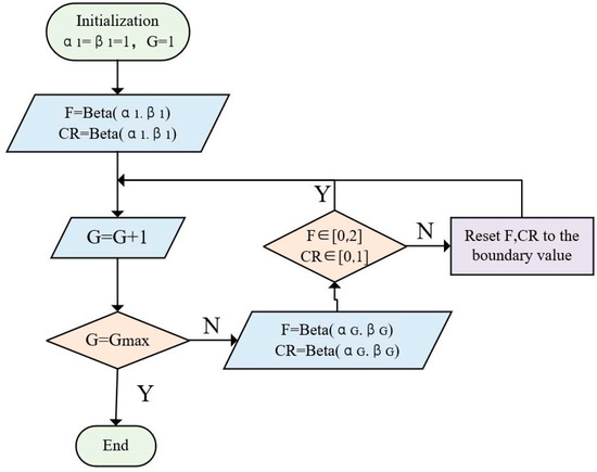
Figure 2.
Calculation process of adaptive and .
4.2. Hybrid Mutation Improvement Strategy
The traditional differential evolution algorithm has limitations in mutation improvement strategies, which limits its versatility. To address this problem, this paper proposes a mutation strategy based on “DE-BB” (differential evolution bare bones) to optimize mutation operations. This strategy is an innovative combination of the backbone particle swarm algorithm and the differential evolution algorithm. Experimental results show that this strategy effectively utilizes the advantages of the backbone particle swarm optimization algorithm in the local depth search, thereby improving the convergence accuracy of the differential evolution algorithm. In the strategy, we incorporate elements of the classic differential mutation and combine them with the adaptive improvement strategy of the F-value to generate individual trial vectors. The specific mutation improvement strategy formula is as follows:
In the formula, are random integers that are different from each other and randomly selected from the population set , and is the scaling factor, where , where is also a random decimal in the interval [0, 1]. is the historical local optimal value of the individual, and is the optimal individual value of the current population.
4.3. Hybrid Cross Improvement Strategy
In traditional differential evolution algorithms, the binomial crossover method (binomial) is often used to cross the contribution vector generated by the mutation operation with the current target vector to generate a test vector . Subsequently, the algorithm competes between the trial vector and the target direction through a greedy selection mechanism, and only the solution vector with better fitness is retained to enter the next round of iteration, while the worse solution vector is eliminated. However, when the contribution vector is already very close to the global optimal position, the crossover operation may destroy its complete solution structure. If the test vector can fully absorb the information of vector , it will help increase the diversity of potential solutions and reduce the risk of the algorithm falling into a local optimum. To this end, this article quotes the crossover strategy of the multi-selection mechanism and combines it with the adaptive improvement strategy of to obtain the crossover improvement strategy formula as follows:
where represents the mixed crossover probability threshold; represents the value of the dimension of individual , calculated by the traditional binomial crossover method. represents the choice probability of performing a binomial crossover or a fully absorbing crossover. According to the experiment of the proposer of this strategy, when the value of parameter is set in the range of [0.4, 0.6], the average convergence speed and convergence accuracy of the algorithm are better than those in other intervals. Therefore, this article sets the parameter to 0.5.
4.4. IADE Algorithm Solution Steps
4.4.1. Codec Strategy
The encoding method used in this article is natural number encoding. Each individual is composed of two chromosomes. The natural number in the first chromosome represents the serial number of the UAV, that is, , where represents the number of monitored vessels; the natural number in the second chromosome represents the serial number of the monitored vessel; that is, also represents the number of monitored vessels. Among them, the upper and lower correspondence between chromosomes represents the vessel to be monitored by the UAV. The chromosome encoding strategy is shown in Figure 3. The UAV with serial number 1 corresponds to the serial number of the monitored vessel {3, 8, 1, 10}, which means that the order of the vessels monitored by UAV No. 1 is {3→8→1→10}.
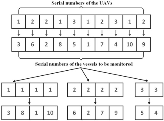
Figure 3.
Chromosome coding strategy.
Decoding requires designing an appropriate decoding solution based on the characteristics of the problem and converting the encoding after the algorithm is executed into the solution to the problem. The specific steps are as follows:
Step 1: According to the order in which each UAV monitors the vessel, consider the UAV endurance time . If, before the UAV goes to the location of the next monitored vessel, , that is, the UAV cannot return to the supply point after monitoring the next vessel, it is necessary to insert a new supply point gene after the gene of the current vessel position, as shown in Figure 4. represents the remaining range of the UAV, represents the distance between the two positions and , represents the current location of the vessel being monitored by the UAV, and represents the position of the next vessel that needs to be monitored, and represents the location of the previous charging point of the UAV; represents the monitoring time.
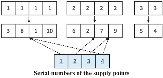
Figure 4.
Replenishment point gene insertion strategy.
Step 2: Select a charging point that meets the conditions for the UAV based on the remaining power of the UAV. If is satisfied, add the current charging point to the gene sequence and add the feasible charging points to the UAV monitoring sequence that is added to the UAV feasible monitoring sequence set , as shown in Figure 4. Finally, a recovery and supply point need to be added at the end of the genetic sequence of each UAV. After the UAV completes its monitoring mission, the mothership is used to recover it.
Step 3: According to the time window constraint in , that is, , select the charging point driving path that meets the mothership speed constraint, as shown in ①→②→⑤ in Figure 5 and the ①→④→⑤ sequence. represents the maximum time point when the UAV reaches supply point and hovers above it, represents the current time point, and represents the speed of the mothership.
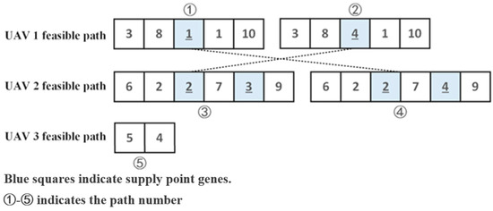
Figure 5.
Viable paths for UAV monitoring.
Step 4: Calculate the total duration of the monitoring task based on the charging point driving path of the mothership, return the fitness function value, and end.
Table 3 gives the solution form of MUCWM path optimization.
Table 3.
Solution form of MUCWM path planning.
4.4.2. Algorithm Process
The process of implementing the IADE algorithm is as follows:
Step 1: Initialize parameters, including population size , extinction coefficient , elite individual replication rate , individual component value range , mutation scaling factor , shape parameters , , crossover probability , mixed crossover probability threshold , the maximum number of iterations .
Step 2: Generate an initial population, with each individual containing parameters, and the value range of the parameters is .
Step 3: Decode the initial population, multiply the first dimension of the individual by , and perform a rounding operation to determine the set of vessels monitored by the UAV. represents the number of UAVs and corresponds to the second-dimension parameters of the individual. Attach a set of sequences to the position, sort the parameters from small to large, retain the attached serial number in the sorting, and use this sorting as the order of the UAV monitoring vessel collection; means the number of vessels to be monitored.
Step 4: Let represent the first iteration.
Step 5: Let represent the first individual.
Step 6: Mutation operation: randomly select 4 individuals , , , and in the population, and generate mutated individuals according to the mixed mutation improvement strategy of Formula (19) .
Step 7: Crossover operation: according to the hybrid crossover improvement strategy of Formula (19), generate new test individuals .
Step 8: Greedy selection: calculate the fitness function value (minimum value of monitoring task completion time); if the fitness function value , update the individual of the previous generation , otherwise the individual of the previous generation is retained.
Step 9: If , let and return to step 5, otherwise go to step 10.
Step 10: Adaptive parameter adjustment. According to the fitness function value, use Formulas (15) and (16) to calculate the adjusted population; use Formula (18) to calculate the adjusted mutation scaling factor and crossover probability .
Step 11: If , , go to step 4, otherwise go to step 11.
Step 12: Output the historical optimal solution and the algorithm ends.
The pseudo-code of the improved adaptive differential evolution algorithm is shown in Algorithm 1.
| Algorithm 1: Improved adaptive differential evolution algorithm |
| 1 Begin |
| 2 Initialize related parameters: , , , , , , , , , |
| 3 Generate initial population |
| 4 Decoding |
| 5 for in |
| 6 for in |
| 7 = The optimal individual and four random individuals generate mutant individuals through Formula (17) |
| 8 Boundary constraint check after mutation |
| 9 = Generate new test individuals through crossover using Formula (18) |
| 10 if then |
| 11 |
| 12 end if |
| 13 end for |
| 14 = Calculate the adjusted population by Formulas (14) and (15) |
| 15 , = scaling factor and crossover probability adaptively adjusted through Formula (16) |
| 16 end for |
| 17 Output the optimal solution , the optimal individual , the algorithm execution time and the algorithm convergence chart |
| 18 Finish |
The flow chart of the algorithm is shown in Figure 6.
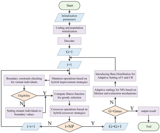
Figure 6.
Flowchart of improved adaptive differential evolution algorithm.
4.5. Algorithm Design for MUCWM Path Optimization Problem
This section mainly describes the basic ideas for solving the MUCWM path optimization problem in three aspects: optimization of UAV monitoring paths, collaboration between motherships and UAVs, and optimization of mothership monitoring paths.
4.5.1. UAV Monitoring Path Optimization
First, the mothership carries multiple UAVs and sets off from the port starting point at the same time. The UAVs will take off from the mothership at the beginning to perform monitoring tasks. At this time, monitoring needs to be planned for multiple UAVs. To achieve this goal, two problems need to be solved: (1) How to determine the collection of UAVs to monitor vessels; (2) how to determine the order of UAVs to monitor vessels.
Ignoring the power constraints of the UAV, that is, treating the UAV power as infinite, we randomly assign vessel collections and monitoring sequences to the UAV. The specific strategy is as follows: First, add an extra dimension sequence to the test individual . Secondly, after multiplying the values of the first dimensional elements of the test individual by respectively, since the value range of the individual elements belongs to , and after rounding off the elements and adding 1, the value range of the first dimension element value of will become , , where is the number of UAVs, and then we sort the second-dimensional elements of from large to small. During the sorting process, the corresponding positions of the additional sequences remain unchanged. Through the above two strategies, the random allocation of the UAV monitoring vessel collection and monitoring sequence is achieved. The random allocation algorithm for UAV monitoring is shown in Algorithm 2.
| Algorithm 2: Random allocation algorithm for UAV monitoring | |
| 1 np.round | |
| 2 np.arangereshape | Generate additional sequences |
| 3 The trial individual formed by appending to the third dimension of | |
| 4 | Count different values in |
| 5 np.unique | |
| 6 for in enumerate | |
| 7 = Split according to the value of unique_values | |
| 8 end for | |
| 9 Sequential allocation strategy for UAV monitoring of vessels: | |
| 10 for in | |
| 11 = Sort according to the value of | |
| 12 end for | |
Figure 7 shows a random allocation strategy in a scenario with 2 UAVs and 5 monitored vessels. The sequence of UAV monitoring vessels is divided into the following: , .
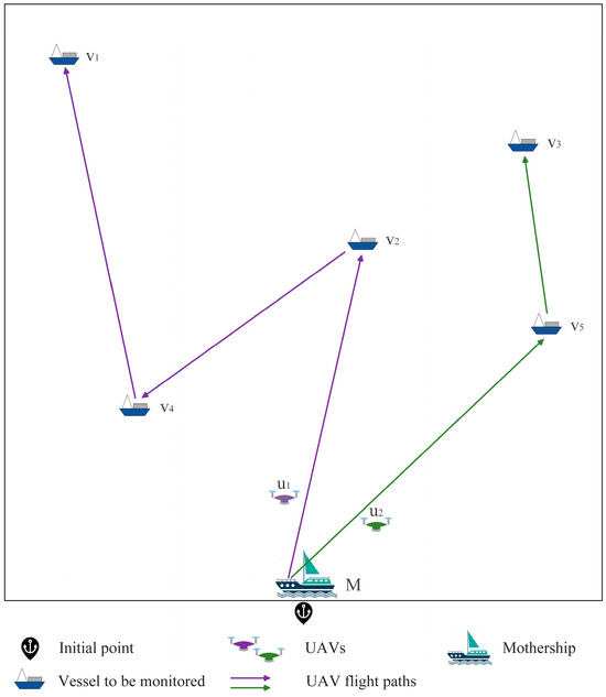
Figure 7.
A random assignment strategy for monitoring vessels by UAVs.
4.5.2. Collaboration between the Mothership and UAVs
Since, in the MUCWM path optimization problem, the mothership plays the role of mobile resupplying for UAVs, this means that the mothership needs to meet the UAVs at the supply point and replenish power for the UAVs in time. Therefore, the mothership and the UAVs need to face the problem of human–machine collaboration, which will be realized based on the selection of UAV power supply points.
First, divide the monitored sea area into equal-area grids, and use the midpoints of all grids as the set of candidate power supply points for UAVs: , where is the divided grid quantity. Based on the value of the individual after the random allocation strategy is executed, and based on the maximum endurance time of the UAV , it is judged whether it is necessary to insert a power supply point for the UAV between the two vessels to be monitored during the monitoring process. Take the UAV in Figure 8 as an example to describe the supply point selection strategy, taking into account the UAV power constraints during the UAV monitoring of vessels.
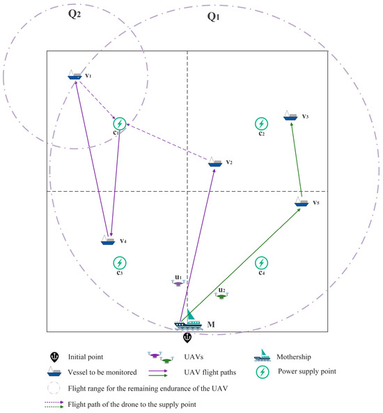
Figure 8.
Synergistic strategy for UAVs and the mothership.
In the initial case, set as the flag that shows that the UAV is fully charged and starts to perform monitoring tasks, and loop through each UAV in sequence; then select the supply points it needs to pass during its voyage. Let ; represents the time consumed by the current UAV to perform the task, loop through the vessel nodes that the UAV needs to monitor, and judge whether it requires the insertion of feasible supply points between two consecutive monitored vessels. The specific strategies are as follows:
(1) Determine whether the vessel node is the first node monitored by the UAV when it departs from the port, that is, whether it meets and at the same time. If the conditions are met, it is judged that the UAV flies to the first node. The vessel node to be monitored will return to the port after monitoring it, that is, will be greater than or equal to , where represents the UAV flight speed; if the conditions are met, the UAV will fly to the location of and monitor it, as shown in Figure 8, the process of UAV flying to . In the algorithm, it is necessary to record the remaining endurance time of the UAV , the UAV monitoring sequence and and set the flag to 0, indicating that the next vessel node is not the first vessel in the UAV monitoring sequence. It is worth mentioning that since the UAV may have multiple candidate power supply points that meet the conditions in subsequent monitoring tasks, the latter node will be calculated from the previous supply point. Therefore, the solution space is an unmanned power supply point. The first monitored vessel node in the UAV monitoring path is a tree structure array with the root as the root. Therefore, the current vessel node is assigned to as the root node of the UAV monitoring path .
(2) Determine whether the next vessel node is the last vessel node in the UAV monitoring sequence. If not, we need to determine whether the UAV can return to the UAV after flying to the next node and monitoring the vessel. Then we determine the last power supply point of the machine, that is, determine whether is greater than or equal to ; if it can, the UAV will fly to the next supply point. In Figure 8, the UAV flies from the location of to the location of for monitoring. The reason for using the above strategy to determine whether the UAV needs to replenish electrical energy is that it must ensure that the UAV has a candidate supply point where it can land. Even if the UAV reaches the next vessel node and completes the monitoring task, the UAV’s remaining power is not satisfied. The recharge point with electric energy constraint can also be returned to the previous recharge point for charging. This strategy ensures that the UAV can land and charge at any point in time and will not run out of power and have nowhere to land during the monitoring mission. If it is not satisfied, it means that the remaining range of the UAV is not enough to support its subsequent monitoring tasks. At this time, all electric energy supply points are traversed, and the unmanned machine selects feasible power supply points. If is greater than or equal to , then is added to the solution of the tree structure, and branches may appear, as shown in Figure 8. The area in , the supply point in the area, represents the position of the supply point that can be reached from the location of the vessel to be monitored under the constraints of UAV endurance. Then we update and . At this time, = + , where represents the charging time of the UAV, and we let flag = 1. Finally, the time consumption from each time the UAV passes through the power supply point is added to the time window set at in order to solve the path planning of the mothership. In Figure 8, the UAV is traveling from the location of the vessel to the vessel . Between the locations, the supply point needs to be inserted. At this time, the next node is the first vessel node monitored by the UAV after it is fully charged and takes off from the mothership; that is, it satisfies flag = = 1 and j > 1. Then it is judged whether the UAV can return to the location of the current supply point after flying to the first vessel node to be monitored and monitoring it, that is, ; if satisfied, then we update and , and set the flag to 0. As shown in Figure 8, the UAV flies from to the vessel node to be monitored.
(3) If the next node is the last node in the UAV monitoring sequence, select an electric energy supply point for the UAV that satisfies the remaining power constraint (recovery point: the UAV will be recovered by the mothership at this node, and the mothership returns to the port together and ends the monitoring task), then is added to the solution of the tree structure, branches may appear, and then , , and are updated. At this time, .
The algorithm for selecting UAV power supply points is shown in Algorithm 3 (the first node time monitored when the UAV takes off from the port).
| Algorithm 3: The algorithm for selecting UAV power supply points | |
| 1 Begin | |
| 2 flag = 1 | |
| 3 for i in | |
| 4 | |
| 5 for j in | |
| 6 | The first node monitored when the UAV takes off from the port |
| 7 if flag = =1 and j = =1 | |
| 8 if | |
| 9 = | |
| 10 = + | |
| 11 | |
| 12 Add to solution structure | |
| 13 end if | |
| 14 end if | |
| 15 end for | |
| 16 end for | |
| 17 Output , , | |
| 18 Finish | |
4.5.3. Mothership Traveling Path Optimization
The results in Section 4.5.2 are used as parameters and input into the optimization algorithm of the mothership monitoring path, which is illustrated in Figure 9. The optimization strategy of the mothership monitoring path is as follows:
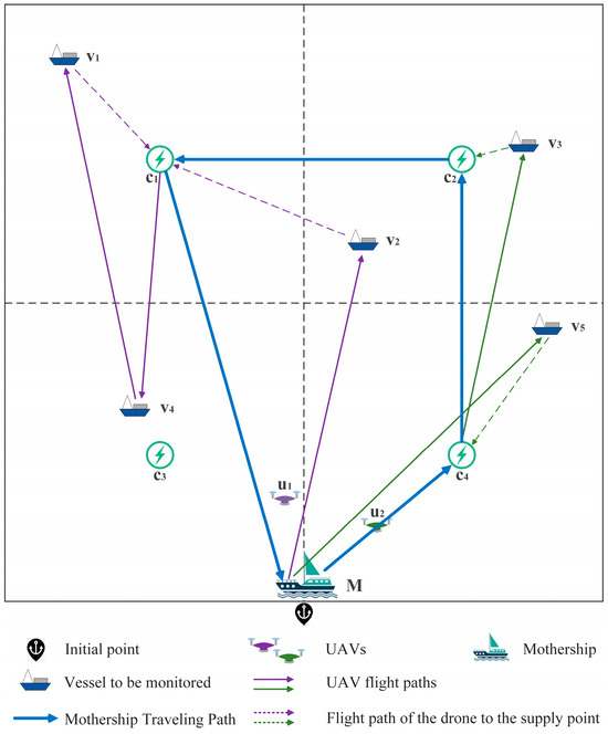
Figure 9.
Monitoring path optimization strategy for the mothership.
(1) First, select one of the feasible monitoring paths of each UAV for calculation. Sort in time order according to to get , which is the sequence in which the mothership passes through each supply point. As shown in Figure 9, the navigation path of the mothership is . Then assign the supply point corresponding to the sorted to the set . Traverse the elements in W, and use the speed constraint of the mothership to determine whether the mothership can reach the corresponding supply point to charge the UAV before the UAV’s power is exhausted, that is, whether is less than ; if satisfied, add to the mothership’s travel path , and update , as shown in Figure 9, each time the mothership moves from the current supply point to the next supply point, such as .
(2) Since the mothership and the UAV can wait for each other at the supply point, it is necessary to determine the order in which the mothership and the UAV arrive at the supply point and then update the time. Specifically, it needs to be judged whether is greater than , where represents the time when the mothership arrives at the supply point. If it is satisfied, it means that the mothership arrived after the UAV arrived at the supply point . At this time, needs to be updated, = , and the UAV waits for the mothership’s time to be added to the time consumption.
(3) After executing a set of data, assign to . represents the completion time of the monitoring task. represents the mothership passing the last supply point. This formula represents the mothership passing through the last supply point. The time when the vessel-borne UAV returns to the port is added to and then assigned to . After all the data have been traversed, the smallest is selected as the optimal solution of the algorithm. Finally, output and .
The pseudocode of the mothership traveling path optimization algorithm is shown in Algorithm 4.
| Algorithm 4: The Mothership Traveling Path Optimization Algorithm |
| 1 Begin |
| 2 Input , , |
| 3 for i in |
| 4 for j in |
| 5 … |
| 6 for n in |
| 7 = Sort in time order according to |
| 8 W = corresponding supply point sequence after sorting |
| 9 = 0 |
| 10 for k in W |
| 11 if < |
| 12 |
| 13 = |
| 14 end if |
| 15 end for |
| 16 + |
| 17 end for |
| 18 … |
| 19 end for |
| 20 end for |
| 21 |
| 22 Output |
| 23 Finish |
5. Experiment and Analysis
In this section, in order to prove the effectiveness of the improved adaptive differential evolution algorithm, this article uses Python 3.12.0 to implement the solution of the algorithm. This experiment was run on a computer with an Intel (R) Core (TM) i5-7200U CPU at 2.50 GHz to 2.70 GHz and a memory of 8 GB.
5.1. Data Preparation and Parameter Settings
This paper conducted a numerical experiment on the vessels entering and leaving the port in a certain port area of Ningbo Zhoushan Port. At 17:40 on 3 April 2023, 100 vessels in the above port were obtained from the automatic identification system (AIS). The position data of vessels sailing in the sea area are partly shown in Table 4. The table gives the vessel serial number, vessel name, vessel type, vessel location (including longitude and latitude), and the update time of the current position. In order to more intuitively display the position of the vessel in the port sea area, a real-time satellite image of the selected sea area is given, as shown in Figure 10. The area within the dotted line is the monitored port sea area.
Table 4.
Data from selected test vessels.
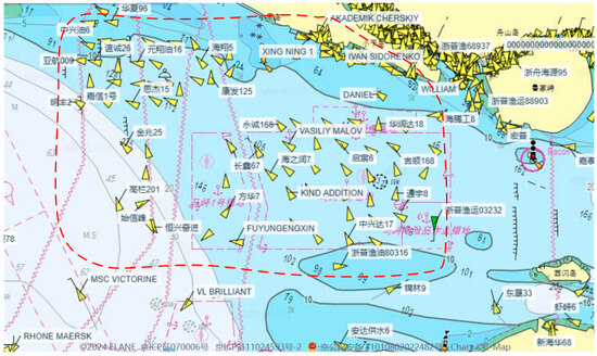
Figure 10.
Schematic diagram of the location of the test vessels in Ningbo Zhoushan Port.
Before parameter setting, we consider some more realistic factors, such as whether the sea state and weather environment have any influence on the path optimization problem of air pollution monitoring of port vessels by shipboard UAVs.
First of all, the performance and stability of the current DJI UAV are very high, and as an example, the wind resistance of the DJI Warp M300 RTK model UAV can reach 12 m/s, i.e., level 6. According to the survey, in some open sea areas, such as the central part of the ocean or some particularly windy sea areas (such as the roaring westerly wind belt in the South Atlantic Ocean), the average wind speed may be between 7 m/s (about 25 km/h) and 10 m/s (about 36 km/h). Wind speeds are somewhat lower in harbor-based waters, so the monitoring mission is largely unaffected by winds at sea. Secondly, wave heights average a few centimeters to 20 m and can only reach 30 m in very extreme natural conditions [49]. However, when monitoring vessels, UAVs need to fly into the vessel’s plume to do so, and the average vessel’s air height (i.e., the height of a vessel in the ocean between sea level and the very top of the vessel) can vary greatly depending on the type and use of the vessel, and the following are the approximate ranges of air heights for some common types of vessels: container vessels: larger container vessels, usually in the range of 40 to 60 m; bulk carriers: medium-sized bulk carriers may be between 20 and 30 m; tankers: roughly between 30 and 50 m; cruise vessels: usually over 50 m; and medium-sized passenger vessels: these are generally between 20 and 30 m. The vessel’s plume is at a position even higher than the highest point of the vessel, so under normal circumstances, the plume height is higher than the waves, and therefore, the UAV monitoring process will not be affected by the waves as long as it maintains the flight height at the plume position.
The default values of the parameters involved in the experiment are shown in Table 5.
Table 5.
Parameter settings involved in the test.
The description of the main parameters in Table 5 is as follows:
Number of UAVs: in the scenario of the vessel exhaust gas measurement trial carried out by the Hanjiang Maritime Safety Department of the Yangzhou Maritime Safety Administration, the number of UAVs was established at three.
Number of equal area divisions in the sea area (number of candidate supply points): In the sea area, it is not advisable to select too many candidate supply points, because too many supply points will greatly increase the running time of the algorithm; at the same time, it is not advisable to select too few candidate supply points, because there may be no solution if there are too few supply points. Therefore, this article divides the sea area into nine equal areas; that is, there are nine candidate supply points.
Port starting point coordinates: set according to the coordinates of a central pier in the port.
Maximum UAV flight speed and maximum UAV endurance time: Based on the UAV produced by DJI that can be used in water conservancy: M300 RTK flight parameters: 55 min maximum flight time, 23 m/s maximum flight speed, and 12 m/s wind resistance. Taking into account the impact of the environment and special circumstances, the maximum flight speed of the UAV is set to 18 m/s, and the maximum endurance time of the UAV is set to 45 min.
Average monitoring time of each vessel: based on previous monitoring experience, the time for UAV monitoring of each vessel is set to 3 min [50].
UAV charging time: In order to save the time required for the total monitoring task, the battery is directly replaced on the mothership to replenish the UAV’s power. Therefore, the battery replacement time is set to 2 min.
The maximum sailing speed of the mothership: Calculated based on the previous average speed of China Maritime Safety Administration port patrol vessels of 20.13 knots. After converting the unit into m/min, it is 621 m/min.
Table 6 shows the parameter settings in the improved adaptive differential evolution algorithm.
Table 6.
Parameterization of improved adaptive differential evolutionary algorithms.
5.2. Solution to MUCWM Path Optimization Algorithm Based on IADE Algorithm
According to the actual geographical location of the port, this article scales the monitored sea area to the plane rectangular coordinate system of 200 × 200 to run the algorithm of this article. Following scaling, the initial positions of the 100 vessels to be monitored, one mothership, and three UAVs were determined, represented by (x, y) coordinates. These data are partially displayed in Table 7. Initially, the three UAVs and the mothership share the same location. Figure 11 visually illustrates the initial locations of the vessels to be monitored, the mothership, and the UAVs.
Table 7.
Partially scaled vessels’ position data.

Figure 11.
Schematic of the vessels’ positions after zooming.
The data are substituted into the improved adaptive differential evolution algorithm to solve the problem. Figure 12 shows the MUCWM path optimization results obtained in the above scenario. Different colors represent different UAV flight paths, and the dotted line is when the UAV goes to the supply point for charging. Since the figure involves many line segments, the path of the mothership will be displayed in the table. Table 8 shows the specific results of path optimization for the mothership and three UAVs.
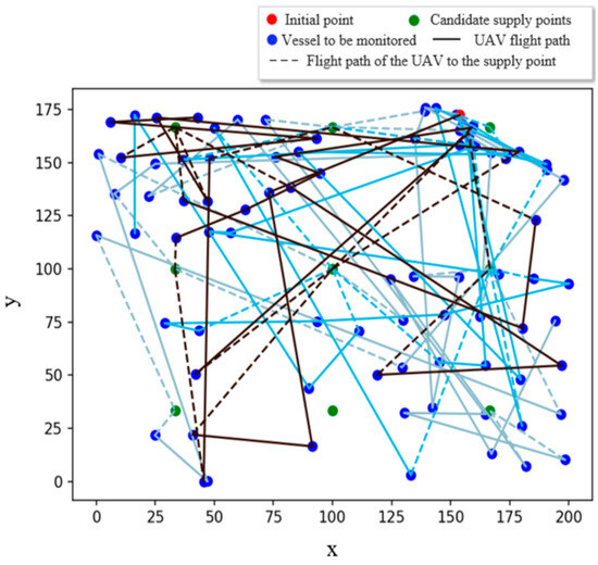
Figure 12.
Schematic diagram of MUCWM path optimization results.
Table 8.
Specific results of MUCWM path optimization.
5.3. Analysis of Results
5.3.1. Algorithm Performance Comparison
In order to verify the accuracy of the algorithm in small-scale calculation examples, the results of IADE solving this problem in small-scale cases are compared with the Gurobi running results. We set the problem scales, , to conduct 12 independent experiments for each scale, and we recorded the GAP between the algorithm and Gurobi in each experiment, where GAP = (f(IADE) − f(Gurobi))/f(Gurobi) × 100%. It is stipulated that if Gurobi runs for more than 30 min and still does not obtain a result, it is considered that Gurobi cannot obtain the solution to the calculation example. The IADE algorithm records the results and running time of each generation and selects the running time of the generation with the smallest difference from the Gurobi result. The comparison results are shown in Table 9.
Table 9.
Experimental comparison of the results of IADE and Gurobi.
It can be seen from the table that, in the independent experiment with , the GAP value between IADE and the accurate result is less than 5%, and the solution speed has been greatly improved. Although Gurobi can obtain accurate results, it takes a long time to solve, so the comparison with the Gurobi results proves the effectiveness of this algorithm in solving the collaborative routing optimization problem of UAVs and motherships, and it has practical application significance in real-life scenarios.
When solving the model, in order to verify the superiority of the improved adaptive differential evolution algorithm compared to the traditional differential evolution algorithm, this paper compares the parameters of the adaptive improved differential evolution algorithm with the basic differential evolution algorithm. The group size and the number of iterations are set to = 100 and = 300, respectively. The resulting operation iteration diagram is shown in Figure 13.
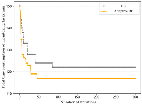
Figure 13.
Adaptive strategy iteration graph.
From Figure 14, it can be seen that the DE algorithm, after the adaptive improvement strategy, shows a trend of being better than the traditional DE algorithm in terms of convergence speed and optimal solution performance.

Figure 14.
Iterative diagram of operator improvement strategy.
On the basis of the adaptive parameter differential evolution algorithm, after adding the hybrid mutation improvement strategy and the hybrid crossover improvement strategy, the test example is also run when = 100 and = 300, and the resulting convergence diagram is shown in Figure 14. It can be seen from the figure that although the convergence speed has dropped slightly, the improved algorithm has strong search capabilities and performs well in manifesting the optimal solution. Therefore, the overall solution performance of the improved adaptive differential evolution algorithm is higher than that of the adaptive differential evolution algorithm.
We took the test case data from Shen et al. [12], as shown in Figure 15, and adjusted the parameters to the values in the article, as shown in Table 10. Since the vessel distribution is relatively concentrated, the number of candidate supply points can be increased to improve the efficiency of the algorithm. Since Shen et al. [12] did not consider the UAV charging time, the UAV charging time was set to 0. Bringing the adjusted data into the algorithm of this article, the result is 116.76982 min, which is smaller than the optimal solution of 126.69466 min in the article. The optimization performance of the improved adaptive differential evolution algorithm is further demonstrated. Figure 16 shows the MUCWM path optimization results obtained by using the algorithm of this article to execute the test case data in Shen et al. [12].

Figure 15.
Test data from Shen et al. [12].
Table 10.
Test data parameter settings.
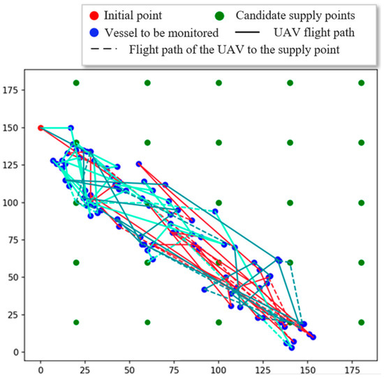
Figure 16.
MUCWM path optimization results for running test data.
5.3.2. Sensitivity Analysis
Figure 17a illustrates that with an increasing number of UAVs, the overall time for MUCWM monitoring decreases, although the rate of reduction in total monitoring time gradually diminishes. Thus, beyond a certain number of UAVs, further increases will not significantly decrease the total duration of the MUCWM monitoring task. Figure 17b reveals that as the number of UAVs grows, the total execution time of the algorithm consistently increases, suggesting a roughly positive correlation between the number of UAVs and the algorithm’s running time.
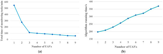
Figure 17.
The relationship between the number of UAVs and the optimal solution and the running time of the algorithm: (a) the relationship between the total time of monitoring tasks and the number of UAVs; (b) the relationship between the algorithm running time and the number of UAVs.
Figure 18a demonstrates that as the number of grid divisions rises, there is a decrease in the total MUCWM monitoring time, particularly noticeable when the grid count increases from 1 to 9. However, with further increases in grid divisions, the rate of reduction in the total monitoring task time starts to taper off. Hence, beyond a certain number of grid divisions, the advantages of further increases in reducing the overall time of the MUCWM monitoring task become marginal. Figure 18b shows that as the number of grid divisions grows, the total execution time of the algorithm also increases, with the rate of increase accelerating, suggesting that the number of grid divisions significantly affects the algorithm’s running time.
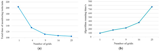
Figure 18.
The relationship between the number of grids and the optimal solution and the running time of the algorithm: (a) the relationship between the total time of monitoring tasks and the number of grids; (b) the relationship between the algorithm running time and the number of grids.
Figure 19 indicates that extending the maximum endurance time of the UAV has a minimal effect on the total duration of the MUCWM monitoring task. This minimal impact is largely due to the introduction of the mothership serving as a mobile power supply for the UAVs, which significantly mitigates the power limitation issues of the UAV. Figure 20 additionally reveals that, while increasing the sailing speed of the mothership reduces the overall monitoring time of MUCWM, this reduction tends to plateau. Thus, after the mothership’s speed reaches a certain level, further increases in speed yield diminishing returns in reducing the total monitoring time. Figure 21 illustrates that, with varying numbers of UAVs, when the number of vessels to be monitored rises from 30 to 150, the algorithm’s running time increases by 2487.962 s. Notably, when the count of vessels monitored in the port surpasses 120, there is a significant spike in the algorithm’s running time. Consequently, the algorithm exhibits improved computational efficiency when the number of vessels monitored remains below 120.
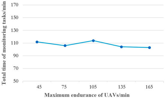
Figure 19.
The relationship between the maximum endurance of UAVs and the total time of monitoring tasks.

Figure 20.
The relationship between the maximum speed of the mothership and the total time of monitoring tasks.

Figure 21.
The relationship between the number of vessels to be monitored and the algorithm running time.
In particular, we discussed the impact on the total monitoring time in the case of leakage of 5–10% of the monitored vessels, and 10 sets of experiments were conducted for each value of leakage, and the results obtained after averaging are shown in Figure 22. From the figure, it can be observed that the total monitoring time tends to decrease as the number of missed vessels increases, and we find that the impact on the total monitoring task is more significant when it is reduced to 10%. This provides a compromise for the port; the port can tradeoff between the time of the total monitoring task and the coverage of the monitored vessels and can choose to give up a small portion of the vessels to obtain a shorter monitoring time, and this analysis provides a certain reference value for the monitoring program of the vessels in the port’s sea area.
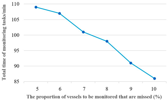
Figure 22.
Relationship between the proportion of vessels to be monitored that are missed and the total time of the monitoring tasks.
6. Conclusions
This paper presents an innovative monitoring solution for vessel air pollution, utilizing a mothership and multiple UAVs to conduct efficient and comprehensive monitoring in maritime pre-monitoring areas. This significantly enhances monitoring efficiency and extends the monitoring scope. The core focus of this research is the path optimization problem for multi-UAV collaborative mothership (MUCWM) monitoring, which encompasses three critical issues: (1) optimizing the monitoring paths of multiple UAVs to ensure efficient and accurate coverage of the target area; (2) developing a collaboration mechanism between the mothership and multiple UAVs to synchronize their monitoring efforts; and (3) optimizing the mothership’s traveling path to maximize overall monitoring efficiency.
To address these challenges, the paper develops a path optimization model for multi-UAV collaborative mothership monitoring of vessel air pollution in port waters. The model is solved using an improved adaptive differential evolution (IADE) algorithm. Utilizing vessel position data from the Automatic Identification System (AIS) of Ningbo Zhoushan Port, we demonstrate the model and algorithm’s effectiveness through an example. Performance comparisons and sensitivity analyses of the algorithm highlight its significant advantages in solving the path planning problems of collaborative operation between the mothership and multiple UAVs.
However, the research also acknowledges certain limitations: the mission optimization model lacks practical constraints such as UAV flight altitude, sea wind speed, and air control. Furthermore, the model designates static supply points as the midpoints of a divided grid network. Future research will explore dynamically adjusting the supply points based on navigation conditions to achieve a better optimal solution.
Author Contributions
Conceptualization, J.S. and L.S.; methodology, J.S.; software, D.Y.; validation, L.S., J.S. and D.Y.; formal analysis, J.S.; data curation, J.S.; writing—original draft preparation, L.S.; writing—review and editing, L.S. All authors have read and agreed to the published version of the manuscript.
Funding
This research was funded by the Liaoning Province Social Science Planning Fund, grant number 2022-ZSK078, the National Natural Science Foundation of China, grant number 72171032, the National Natural Science Foundation of China, grant number 71702019, and the Humanities and Social Science Foundation of the Ministry of Education, grant number 21YJAZH070.
Institutional Review Board Statement
Not applicable.
Informed Consent Statement
Not applicable.
Data Availability Statement
All data are available in the paper.
Conflicts of Interest
The authors declare no conflicts of interest. The funders had no role in the design of the study; in the collection, analyses, or interpretation of data; in the writing of the manuscript; or in the decision to publish the results.
References
- Sun, Z.H.; Luo, X.; Wu, E.Q.; Zuo, T.Y.; Tang, Z.R.; Zhuang, Z. Monitoring Scheduling of Drones for Emission Control Areas: An Ant Colony-Based Approach. IEEE Trans. Intell. Transp. Syst. 2021, 23, 11699–11709. [Google Scholar] [CrossRef]
- Sirimanne, S.N.; Hoffman, J.; Juan, W.; Asariotis, R. Review of Maritime Transport 2019; United Nations: New York, NY, USA, 2019; Volume 9. [Google Scholar]
- United Nations. Review of Maritime Transport 2023: United Nations Conference on Trade and Development. 2023. Available online: https://unctad.org/publication/review-maritime-transport-2023 (accessed on 27 September 2023).
- Liang, G.Y. Neglected pollution sources. Environment 2016, 6, 17–19. [Google Scholar]
- Transport & Environment, Air Pollution from Ships. 2018. Available online: https://www.transportenvironment.org/articles/air-pollution-ships (accessed on 20 January 2018).
- Li, L.; Gao, S.; Yang, W. The enforcement of ECA regulations: Inspection strategy for on-board fuel sampling. J. Comb. Optim. 2022, 44, 2551–2576. [Google Scholar] [CrossRef]
- Sun, P.Z.; Luo, X.; Zuo, T.; Bao, Y.; Sun, Y.N.; Law, R.; Wu, E.Q. Emission Monitoring Dispatching of Drones Under Vessel Speed Fluctuation. IEEE Trans. Intell. Transp. Syst. 2022, 23, 21833–21847. [Google Scholar] [CrossRef]
- Xia, J.; Wang, K.; Wang, S. Drone scheduling to monitor vessels in emission control areas. Transp. Res. Part B Methodol. 2019, 119, 174–196. [Google Scholar] [CrossRef]
- IMO Low Sulfur Fuel Emission Control Partial State Requirements. 2018. Available online: https://www.sohu.com/a/284957167_120015135 (accessed on 27 December 2018).
- China MSA. The Latest Global Emission Control Areas and Low-Sulfur Oil Areas Data Collation and Sink. 2022. Available online: http://www.360doc.com/content/22/0823/07/77972649_1044930083.shtml (accessed on 23 August 2022).
- OECD. Reducing Sulphur Emissions from Ships. 2018. Available online: https://www.oecd-ilibrary.org/transport/reducing-sulphur-emissions-from-ships_5jlwvz8mqq9s-en (accessed on 20 January 2018).
- Shen, L.; Hou, Y.; Yang, Q.; Lv, M.; Dong, J.X.; Yang, Z.; Li, D. Synergistic path planning for ship-deployed multiple UAVs to monitor vessel pollution in ports. Transp. Res. Part D Transp. Environ. 2022, 110, 103415. [Google Scholar] [CrossRef]
- Stein, M. Conducting safety inspections of container gantry cranes using Unmanned Aerial Vehicles. In Dynamics in Logistic, Proceedings of the 6th International Conference LDIC 2018, Bremen, Germany, 20–22 February 2018; Springer International Publishing: Cham, Switzerland, 2018; pp. 154–161. [Google Scholar]
- Urbahs, A.; Zavtkevics, V. Oil pollution monitoring of sea aquatorium features with using unmanned aerial vehicles. In Proceedings of the 17th International Conference Transport Means, Kaunas, Lithuania, 23–24 October 2014; pp. 75–78. [Google Scholar]
- Zhang, S.; Xin, M.; Wang, X.; Zhang, M. Anchor-free network with guided attention for ship detection in aerial imagery. J. Appl. Remote Sens. 2021, 15, 024511. [Google Scholar] [CrossRef]
- Primeau, N.; Abielmona, R.; Falcon, R.; Petriu, E. Maritime smuggling detection and mitigation using risk-aware hybrid robotic sensor networks. In Proceedings of the 2017 IEEE Conference on Cognitive and Computational Aspects of Situation Management (CogSIMA), Savannah, GA, USA, 27–31 March 2017; pp. 1–7. [Google Scholar]
- Kim, J.S.; Lee, M.J.; Nam, H.; Do, S.; Lee, J.H.; Park, M.K.; Park, B.H. Indoor and Outdoor Tests for a Chemi-capacitance Carbon Nanotube Sensor Installed on a Quadrotor Unmanned Aerial Vehicle for Dimethyl Methylphosphonate Detection and Mapping. ACS Omega 2021, 6, 16159–16164. [Google Scholar] [CrossRef] [PubMed]
- Soarabolity. How does UAV Estimate the Sulfur Content of Ship Fuel by Monitoring Ship Exhaust [EB/OL]. Available online: https://www.sohu.com/a/399172599_100226347 (accessed on 2 June 2020).
- Flyable technology Soarability. Maritime Administration Explores Implementation of Drone Ship Exhaust Monitoring. 2022. Available online: https://baijiahao.baidu.com/s?id=1738314327938212810&wfr=spider&for=pc (accessed on 14 July 2022).
- Jiangsu Maritime Bureau of the People’s Republic of China, News Events. 2022. Available online: https://www.js.msa.gov.cn/art/2022/7/11/art_47_1356157.html (accessed on 11 July 2022).
- China seShipping. Port of Rotterdam Is Trialling New Drones to Monitor Ship Emissions. 2022. Available online: https://www.chineseshipping.com.cn/cninfo/News/202210/t20221021_1370484.shtml (accessed on 21 October 2022).
- Explanation of the Endurance of Multi-Rotor Drones and Fixed-Wing Drones. Military/Avionics. 2023. Available online: https://m.elecfans.com/article/2238023.html (accessed on 7 September 2023).
- Murray, C.C.; Chu, A.G. The flying sidekick traveling salesman problem: Optimization of drone-assisted parcel delivery. Transp. Res. Part C Emerg. Technol. 2015, 54, 86–109. [Google Scholar] [CrossRef]
- Agatz, N.; Bouman, P.; Schmidt, M. Optimization approaches for the traveling salesman problem with drone. Transp. Sci. 2018, 52, 965–981. [Google Scholar] [CrossRef]
- Bouman, P.; Agatz, N.; Schmidt, M. Dynamic programming approaches for the traveling salesman problem with drone. Networks 2018, 72, 528–542. [Google Scholar] [CrossRef]
- Ha, Q.M.; Deville, Y.; Pham, Q.D.; Hà, M.H. On the min-cost traveling salesman problem with drone. Transp. Res. Part C Emerg. Technol. 2018, 86, 597–621. [Google Scholar] [CrossRef]
- Yurek, E.E.; Ozmutlu, H.C. A decomposition-based iterative optimization algorithm for traveling salesman problem with drone. Transp. Res. Part C Emerg. Technol. 2018, 91, 249–262. [Google Scholar] [CrossRef]
- Tu, P.A.; Dat, N.T.; Dung, P.Q. Traveling salesman problem with multiple drones. In Proceedings of the 9th International Symposium on Information and Communication Technology, Da Nang, Vietnam, 6–7 December 2018; pp. 46–53. [Google Scholar]
- Wang, X.; Poikonen, S.; Golden, B. The vehicle routing problem with drones: Several worst-case results. Optim. Lett. 2017, 11, 679–697. [Google Scholar] [CrossRef]
- Poikonen, S.; Wang, X.; Golden, B. The vehicle routing problem with drones: Extended models and connections. Networks 2017, 70, 34–43. [Google Scholar] [CrossRef]
- Kitjacharoenchai, P.; Lee, S. Vehicle routing problem with drones for last mile delivery. Procedia Manuf. 2019, 39, 314–324. [Google Scholar] [CrossRef]
- Dayarian, I.; Savelsbergh, M.; Clarke, J.P. Same-day delivery with drone resupply. Transp. Sci. 2020, 54, 229–249. [Google Scholar] [CrossRef]
- Karak, A.; Abdelghany, K. The hybrid vehicle-drone routing problem for pick-up and delivery services. Transp. Res. Part C Emerg. Technol. 2019, 102, 427–449. [Google Scholar] [CrossRef]
- Poikonen, S.; Golden, B. Multi-visit drone routing problem. Comput. Oper. Res. 2020, 113, 104802. [Google Scholar] [CrossRef]
- Guerriero, F.; Surace, R.; Loscri, V.; Natalizio, E. A multi-objective approach for unmanned aerial vehicle routing problem with soft time windows constraints. Appl. Math. Model. 2014, 38, 839–852. [Google Scholar] [CrossRef]
- Phan, D.H.; Suzuki, J. Evolutionary multiobjective optimization for the pickup and delivery problem with time windows and demands. Mob. Netw. Appl. 2016, 21, 175–190. [Google Scholar] [CrossRef]
- Schermer, D.; Moeini, M.; Wendt, O. A matheuristic for the vehicle routing problem with drones and its variants. Transp. Res. Part C Emerg. Technol. 2019, 106, 166–204. [Google Scholar] [CrossRef]
- Wang, Z.; Sheu, J.B. Vehicle routing problem with drones. Transp. Res. Part B Methodol. 2019, 122, 350–364. [Google Scholar] [CrossRef]
- Sacramento, D.; Pisinger, D.; Ropke, S. An adaptive large neighborhood search metaheuristic for the vehicle routing problem with drones. Transp. Res. Part C Emerg. Technol. 2019, 102, 289–315. [Google Scholar] [CrossRef]
- Zajac, S.; Huber, S. Objectives and methods in multi-objective routing problems: A survey and classification scheme. Eur. J. Oper. Res. 2021, 290, 1–25. [Google Scholar] [CrossRef]
- Qin, W.; Shi, Z.; Li, W.; Li, K.; Zhang, T.; Wang, R. Multiobjective routing optimization of mobile charging vehicles for UAV power supply guarantees. Comput. Ind. Eng. 2021, 162, 107714. [Google Scholar] [CrossRef]
- Yu, K.; Budhiraja, A.K.; Tokekar, P. Algorithms for routing of unmanned aerial vehicles with mobile recharging stations and for package delivery. arXiv 2017, arXiv:1704.00079. [Google Scholar]
- Zhu, K.; Yang, J.; Zhang, Y.; Nie, J.; Lim, W.Y.B.; Zhang, H.; Xiong, Z. Aerial refueling: Scheduling wireless energy charging for UAV enabled data collection. IEEE Trans. Green Commun. Netw. 2022, 6, 1494–1510. [Google Scholar] [CrossRef]
- Zhou, Y.; Cheng, N.; Lu, N.; Shen, X.S. Multi-UAV-aided networks: Aerial-ground cooperative vehicular networking architecture. IEEE Veh. Technol. Mag. 2015, 10, 36–44. [Google Scholar] [CrossRef]
- Luo, Z.; Liu, Z.; Shi, J. A two-echelon cooperated routing problem for a ground vehicle and its carried unmanned aerial vehicle. Sensors 2017, 17, 1144. [Google Scholar] [CrossRef]
- Shen, L.; Wang, Y.; Liu, K.; Yang, Z.; Shi, X.; Yang, X.; Jing, K. Synergistic path planning of multi-UAVs for air pollution detection of ships in ports. Transp. Res. Part E Logist. Transp. Rev. 2020, 144, 102128. [Google Scholar] [CrossRef]
- Yuan, H.; Xiao, C.; Wang, Y.; Peng, X.; Wen, Y.; Li, Q. Maritime vessel emission monitoring by an UAV gas sensor system. Ocean. Eng. 2020, 218, 108206. [Google Scholar] [CrossRef]
- Luo, X.; Sun, Z.H.; Qiu, S. Ant colony system based drone scheduling for ship emission monitoring. In Proceedings of the 2021 IEEE Congress on Evolutionary Computation (CEC), Kraków, Poland, 28 June–1 July 2021; pp. 241–247. [Google Scholar]
- Drones for Ship Exhaust Monitoring, DroneNet. Available online: https://www.163.com/dy/article/IEOJKCVR05149OCK.html (accessed on 16 September 2023).
- Sea Wave. Key Laboratory of Coastal Disaster and Protection (Hohai University), Ministry of Education. 2019. Available online: https://coast.hhu.edu.cn/2020/0512/c2585a203485/page.htm (accessed on 11 November 2019).
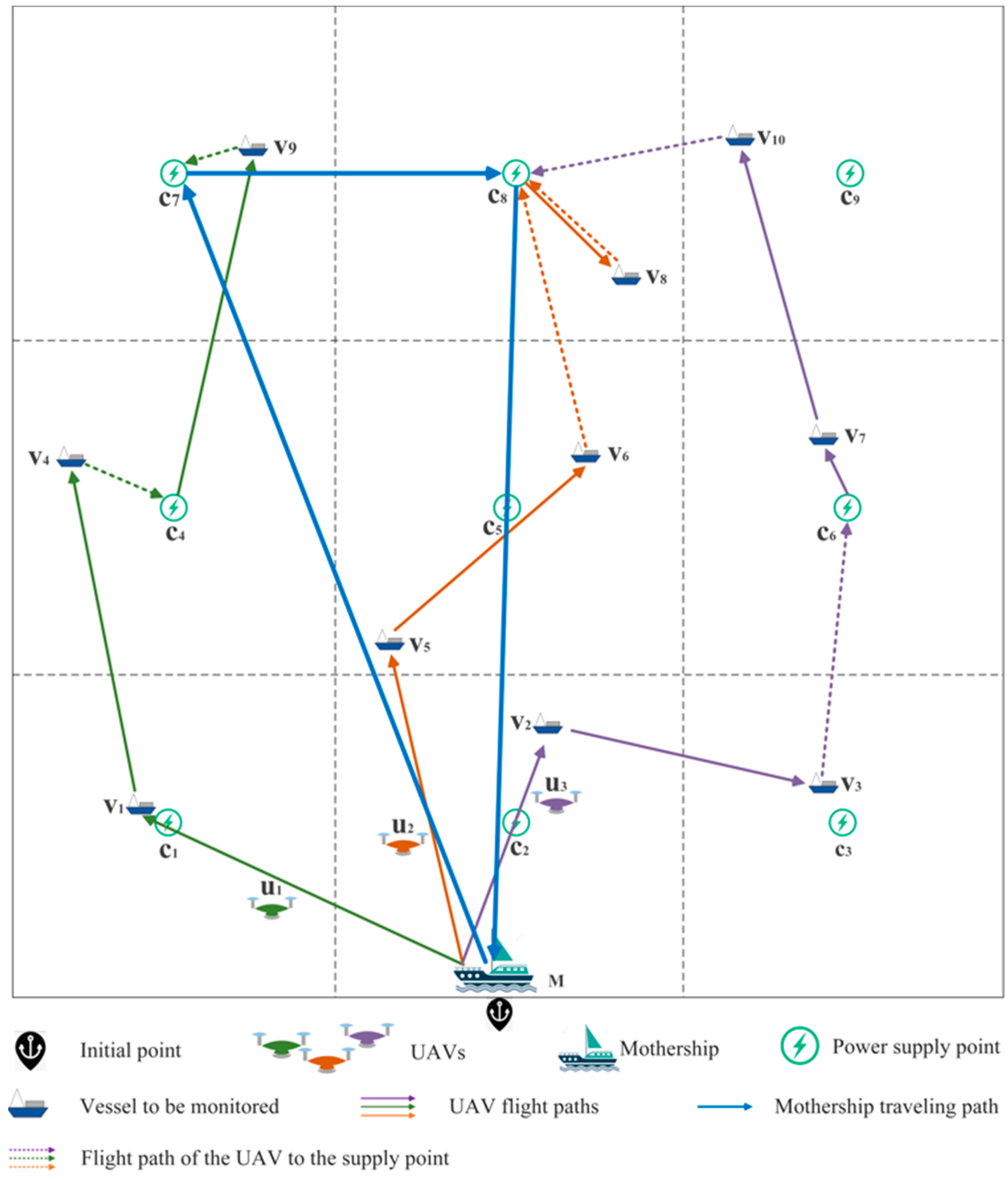
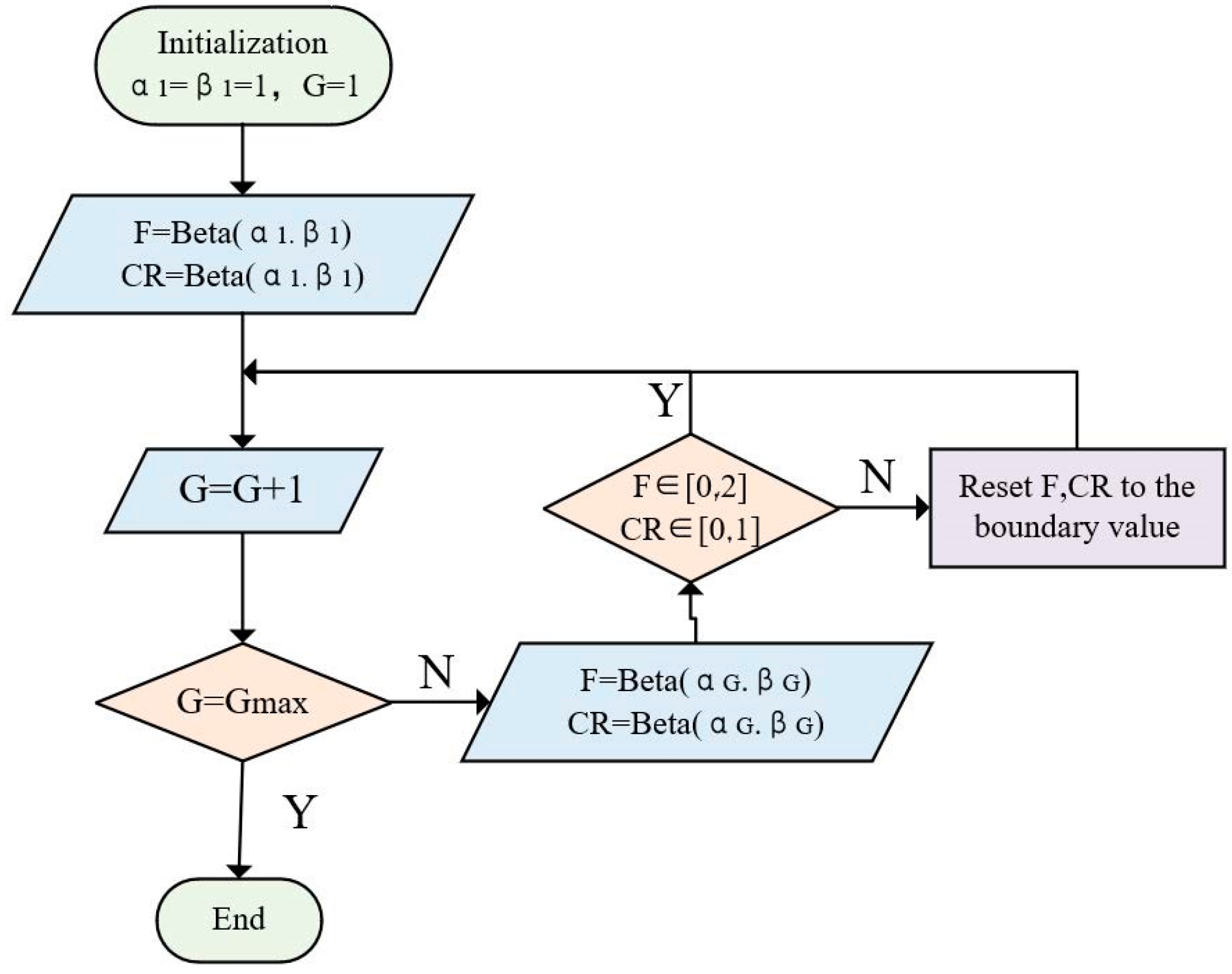
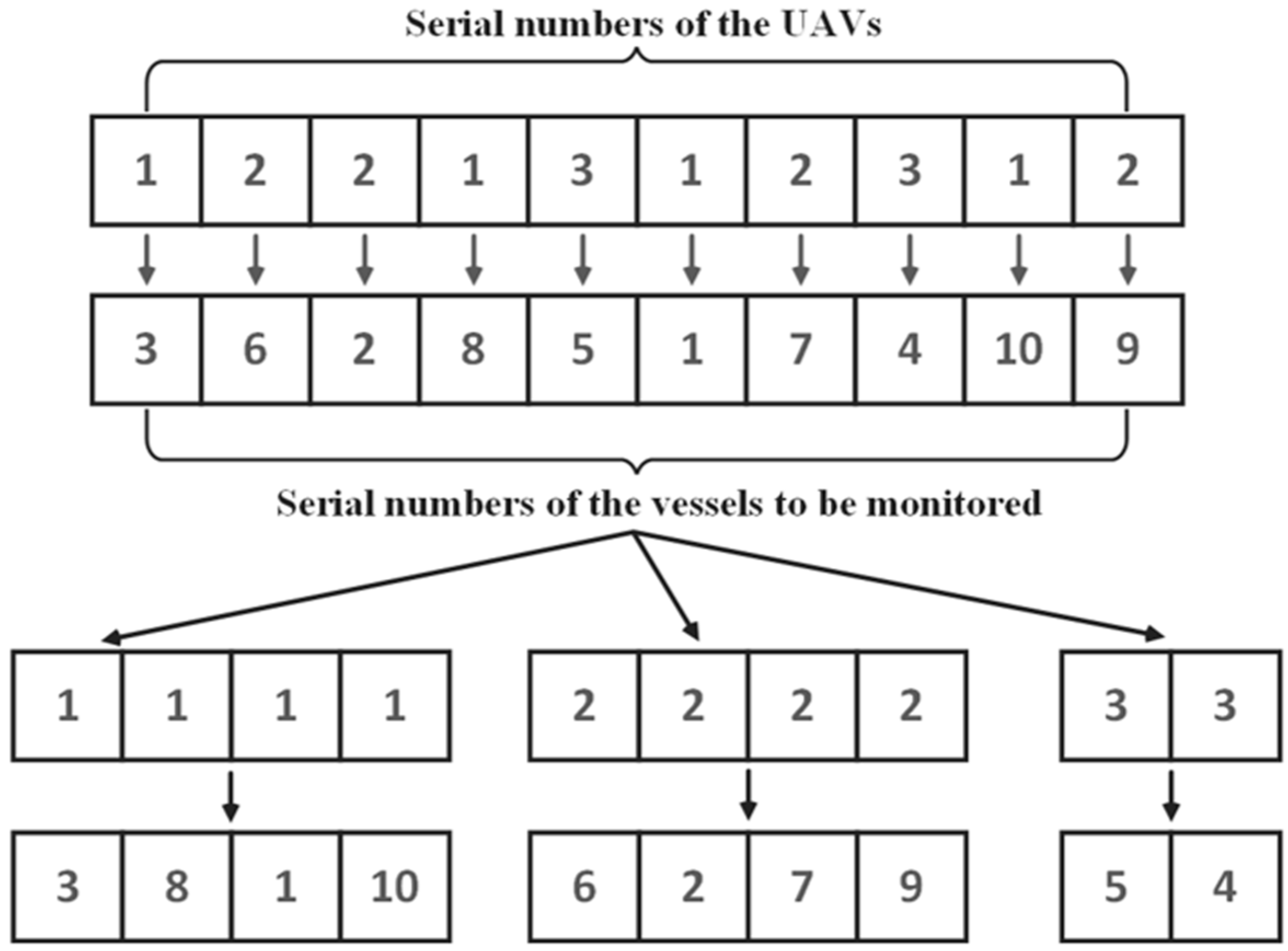
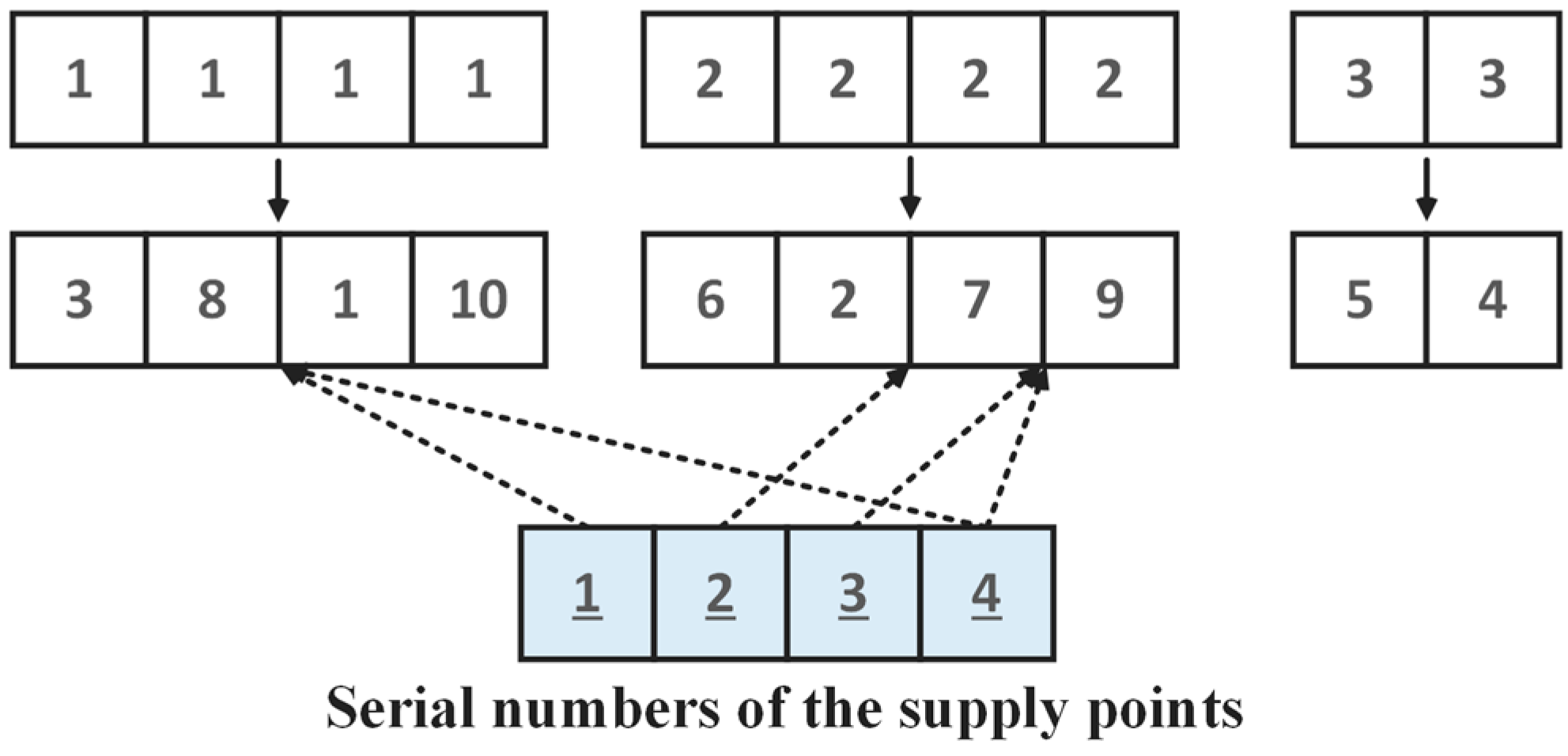
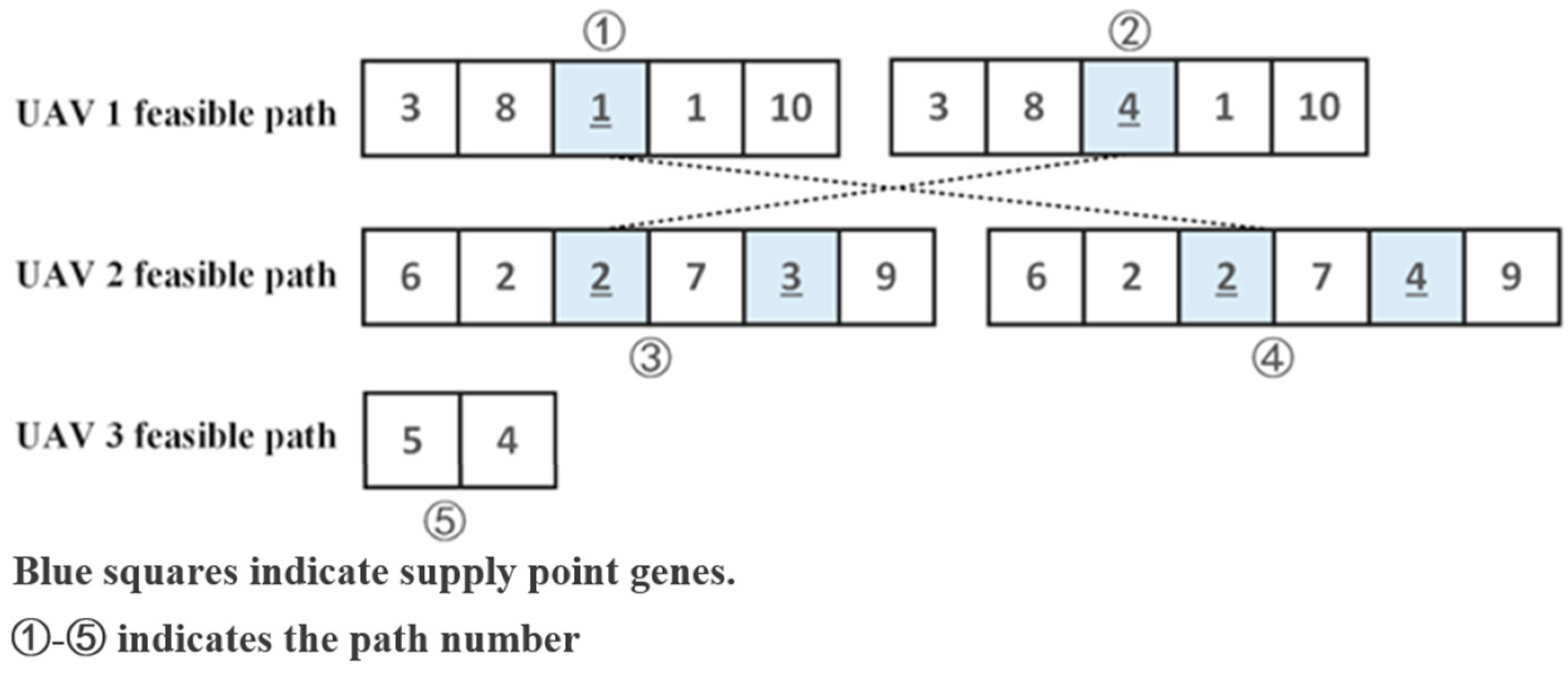
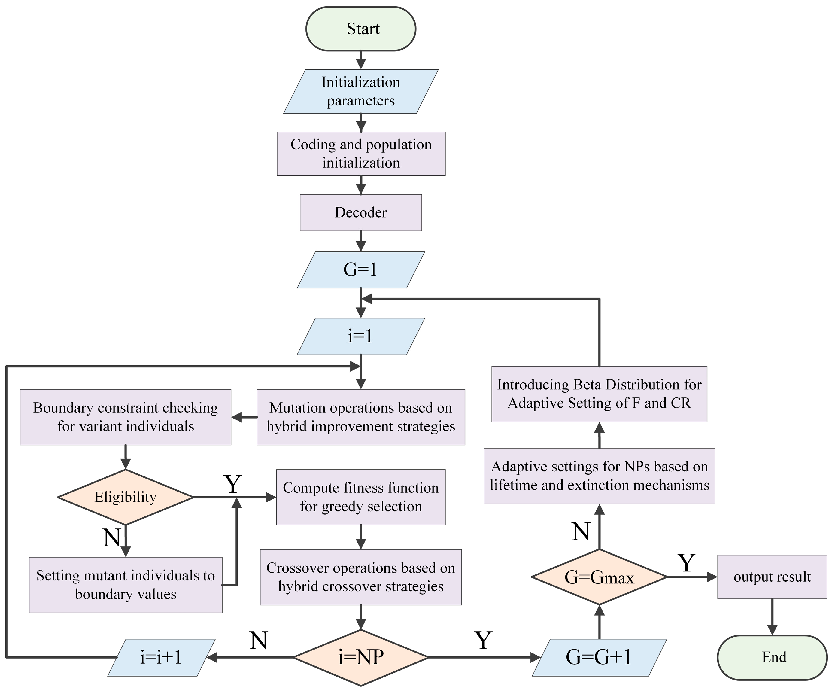

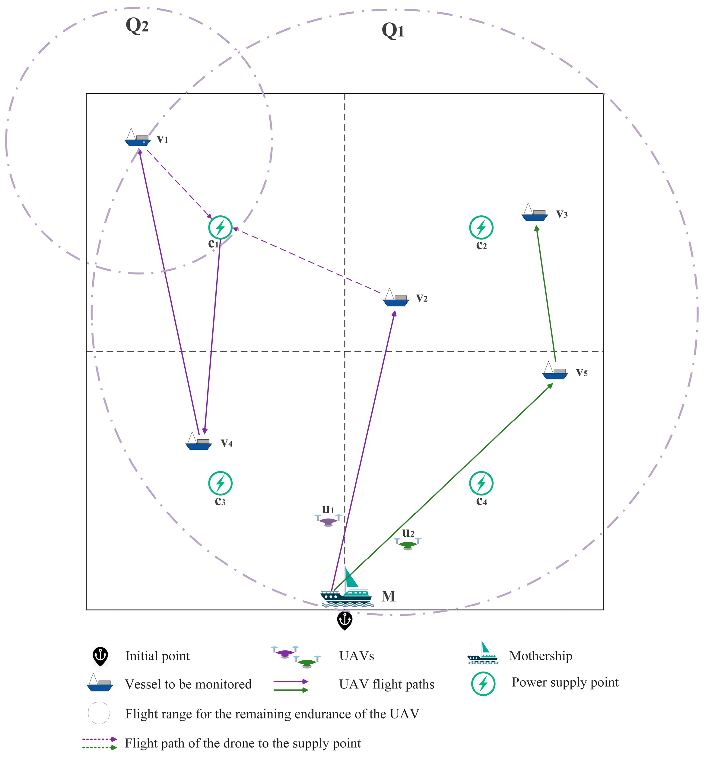
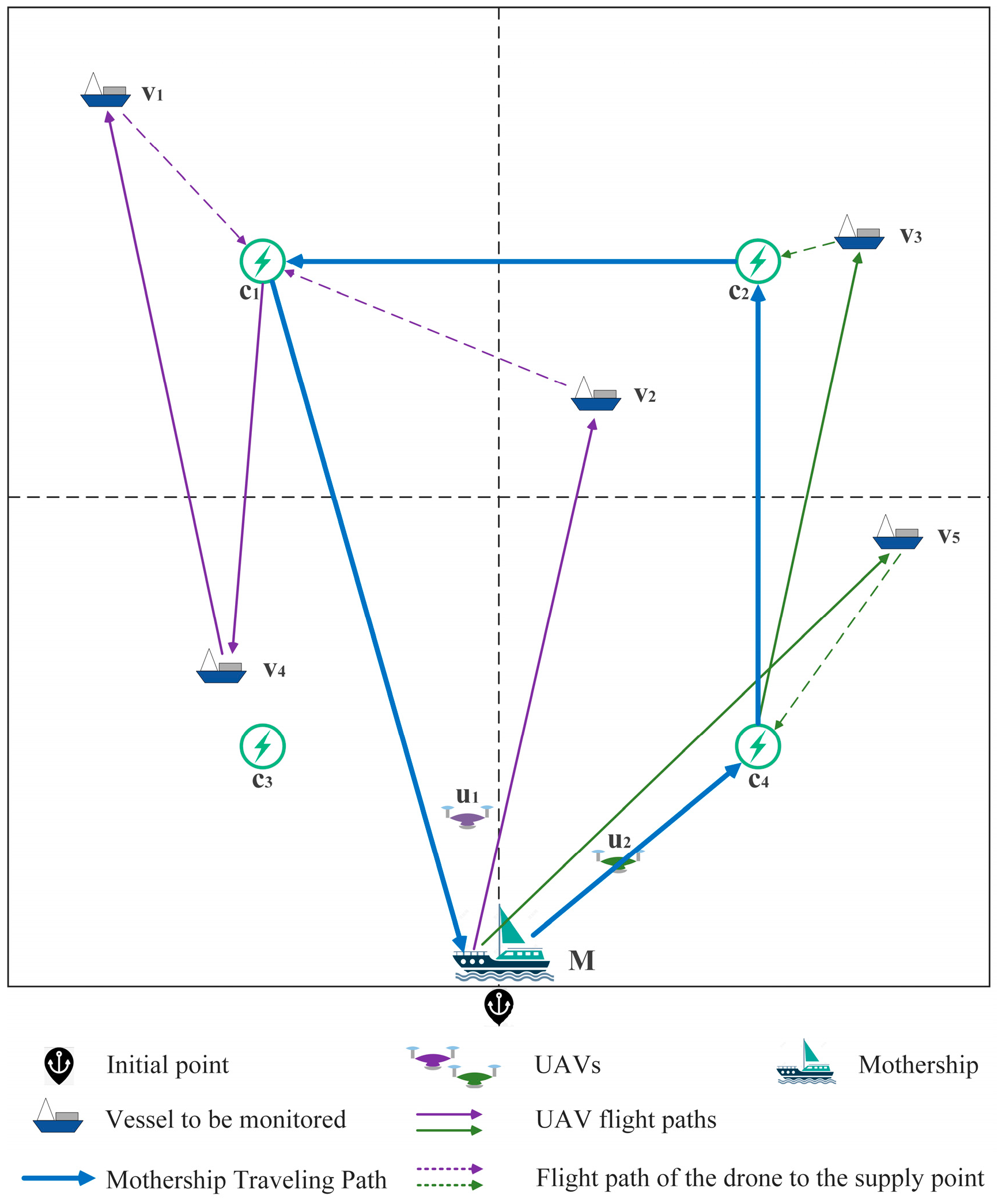

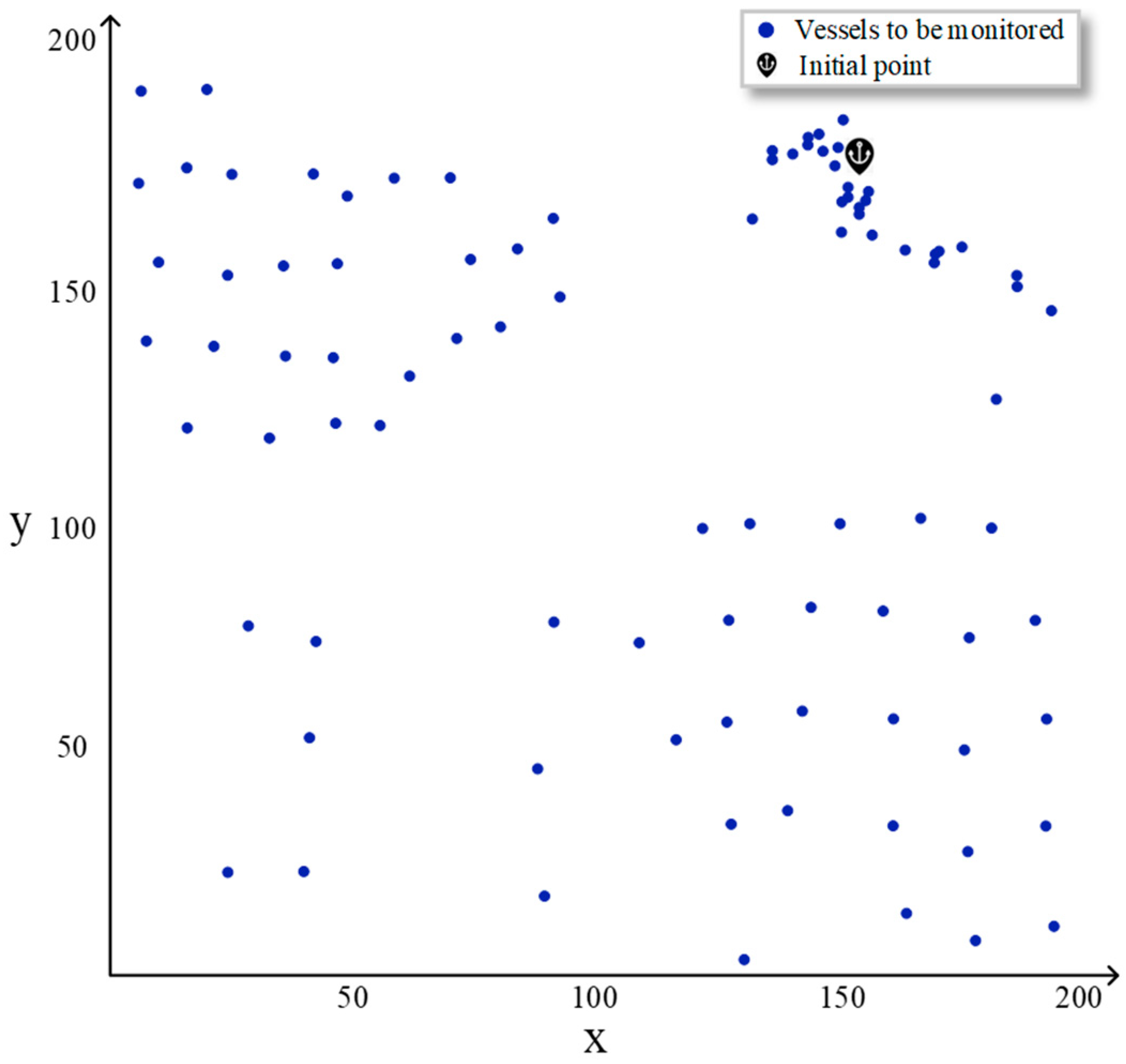
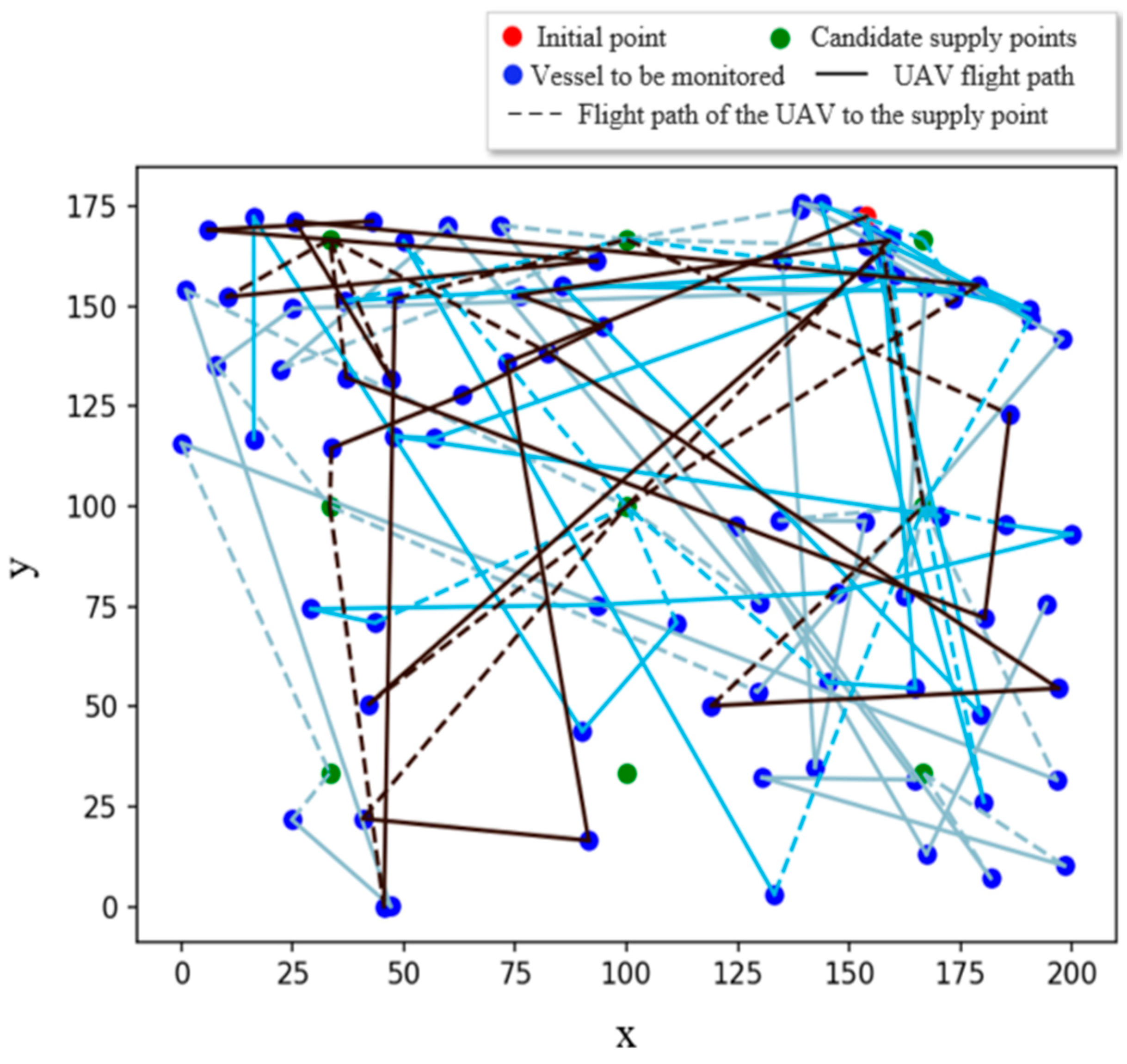
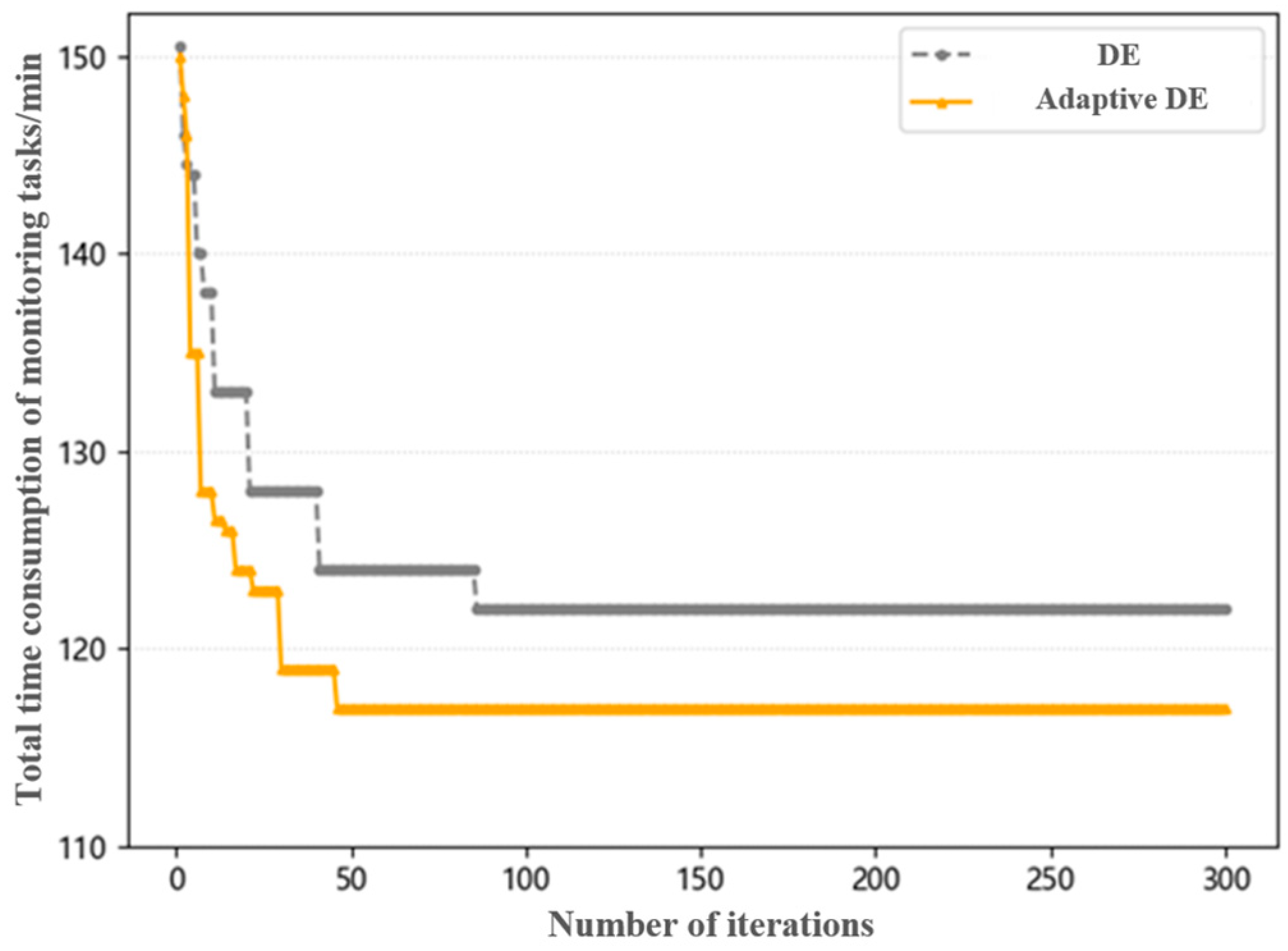
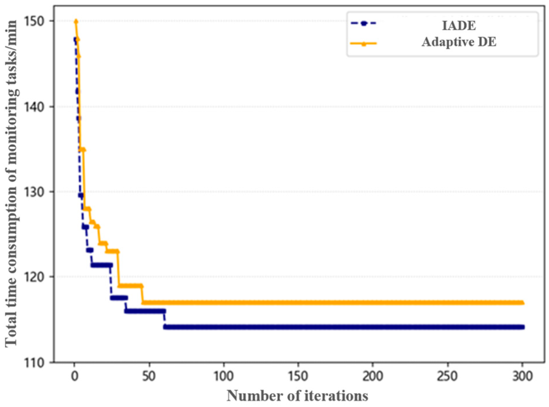
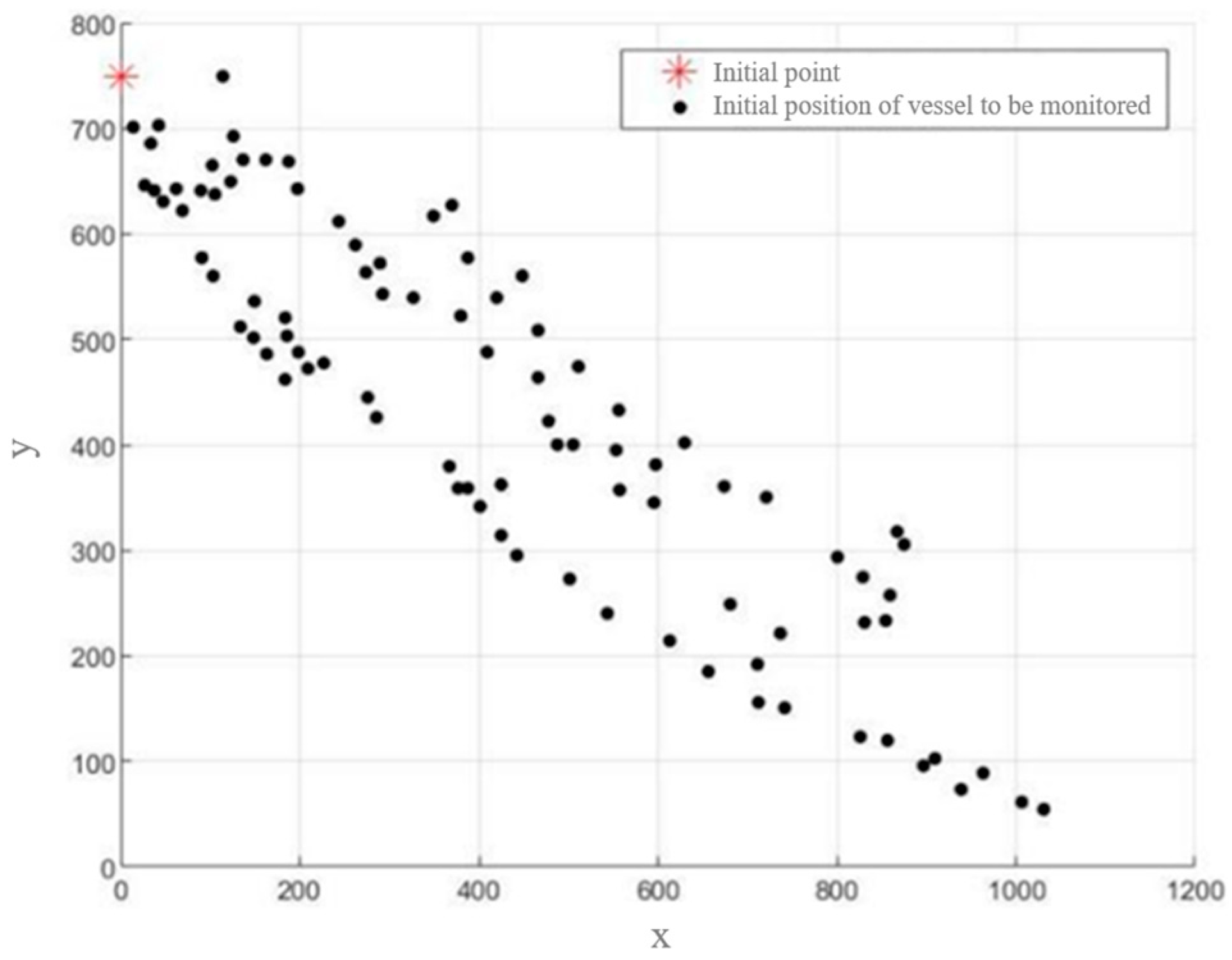
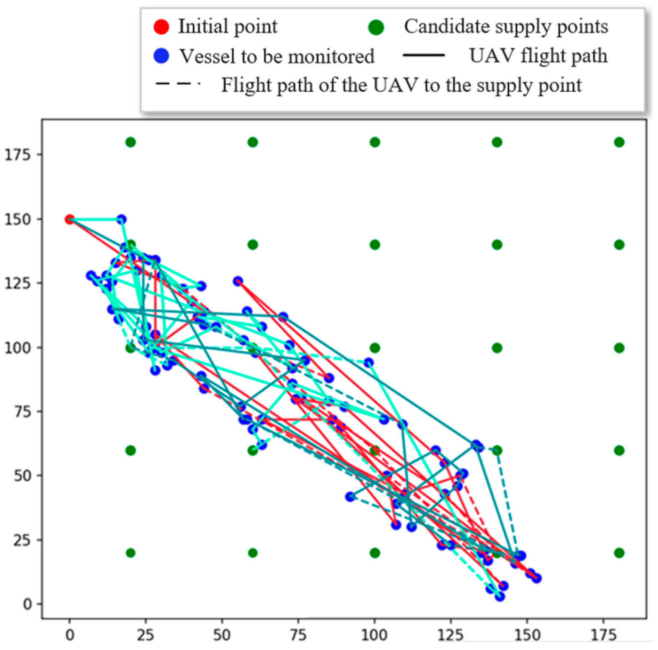
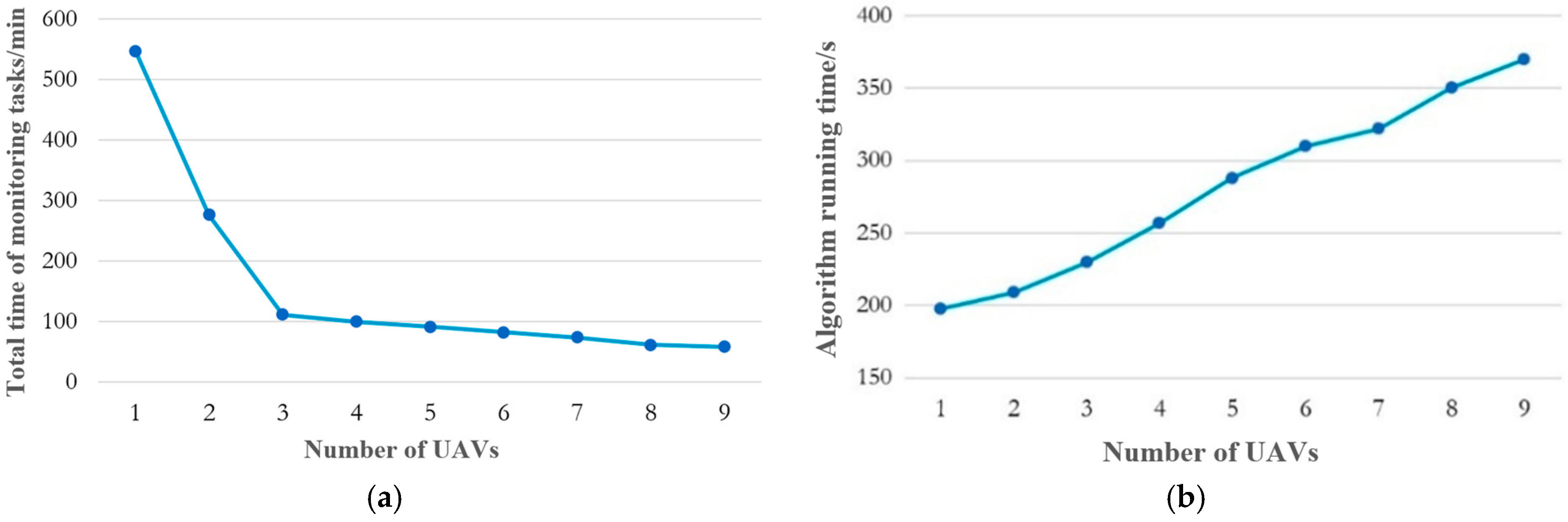
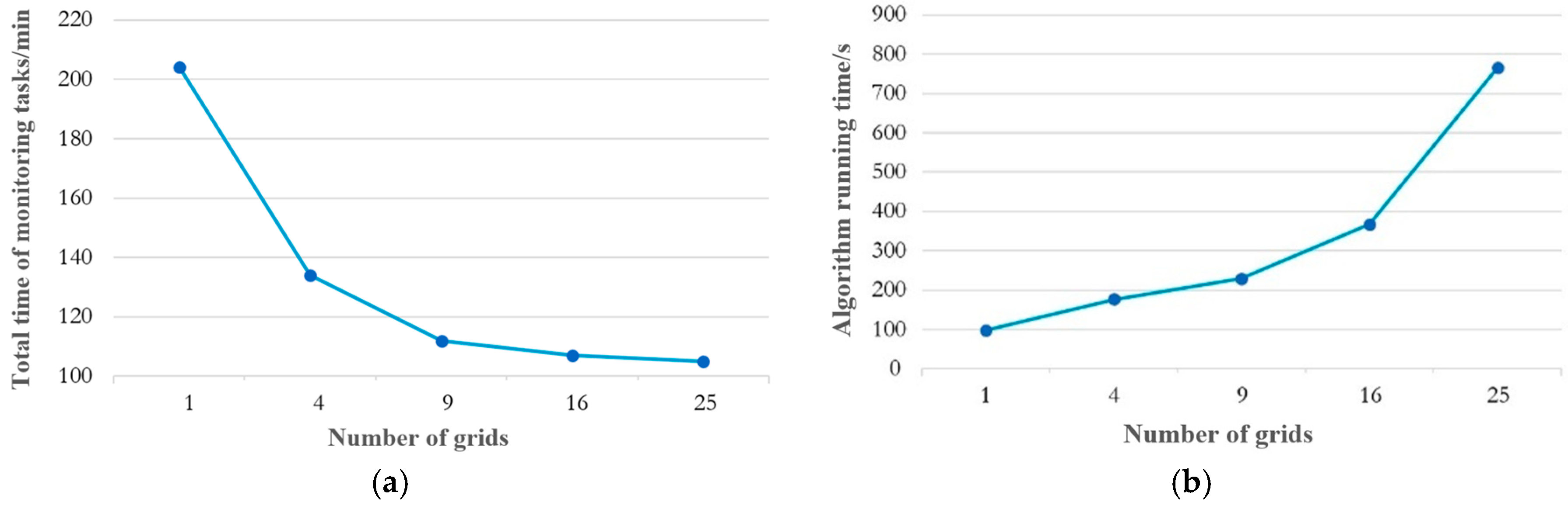

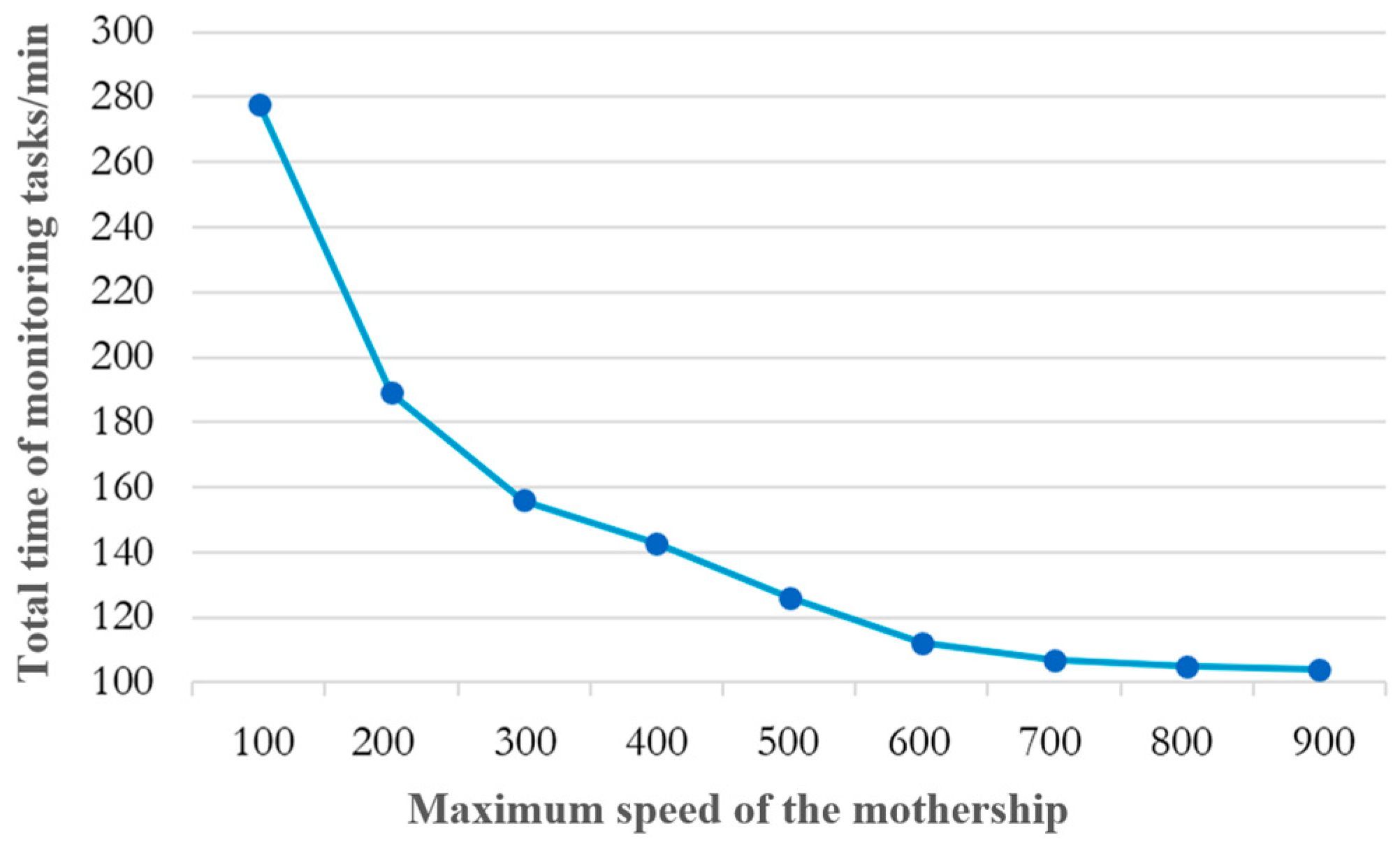
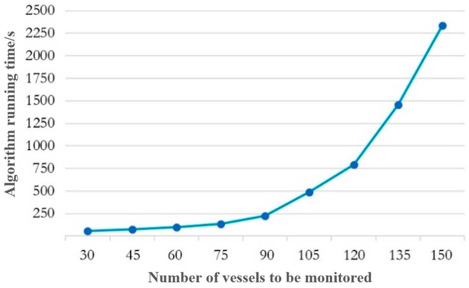

Disclaimer/Publisher’s Note: The statements, opinions and data contained in all publications are solely those of the individual author(s) and contributor(s) and not of MDPI and/or the editor(s). MDPI and/or the editor(s) disclaim responsibility for any injury to people or property resulting from any ideas, methods, instructions or products referred to in the content. |
© 2024 by the authors. Licensee MDPI, Basel, Switzerland. This article is an open access article distributed under the terms and conditions of the Creative Commons Attribution (CC BY) license (https://creativecommons.org/licenses/by/4.0/).