Abstract
Mobility as a service, and its associated variants, has been proposed as a method to improve the sustainability of transport systems; however, most of the approaches that have been proposed so far have been unsuccessful or have worsened the situation. The work presented in this paper investigates an intermodal system that combines a ride-pooling service with a public transport network. The system is composed of a dedicated simulator that evaluates the transport scenario and an intermodal dispatcher that optimises the service according to requests, accounting for their time windows. This intermodal approach considers trips with multiple legs, for which either ride-pooling or public transport are used. This study investigates how the batch size and the early dispatching of the last leg, supported by a vehicle reservation strategy, impact diverse demand profiles that range from single-passenger to multiple-passenger requests, while also addressing the critical aspect of fleet size. The experimental setting used in this work is the metropolitan area of Barcelona; the experimentation results yield valuable insights into the functionality of the proposed intermodal system.
1. Introduction
There are various forms of shared mobility, including the concept of mobility as a service (MaaS). Although initially appearing to offer a potential solution to congestion problems in large cities, studies conducted by [1,2,3] have revealed unexpected consequences such as increased travel times and reduced public transport usage. To foster beneficial outcomes for citizens, the International Association of Public Transport (UITP, as per the acronym in French) emphasises the need for complementarity rather than competition within public transportation, aiming for win–win scenarios [4].
From the point of view of the prospective application and development of newly conceived and innovative urban transportation systems related to on-demand transport and public transportation networks, the research reported in [5] provides some initial insights and sparks the idea of using shared services to feed public transport whenever possible. Various studies, such as those conducted by the International Transport Forum (ITF) for cities like Lisbon, Helsinki, Auckland and Dublin (e.g., [6,7,8]), analyse how including ride-pooling services can incentivise individuals to shift from private vehicles to this alternative transport mode without undermining public transport. It must be remarked that these are simulation studies and not empirical studies, referring to a system with a substantially different structure from the one tackled in this paper. For empirical research directly related to the type of intermodal system to which our paper applies, no research has been found; as to our knowledge, this intermodal system has not yet been put into operation. Moreover, the recent bankruptcy of MaaS Global, a pioneer in the MaaS concept, highlights the challenges faced by such initiatives in achieving commercial sustainability [9]. This underscores the importance for studies to include a profitability analysis to assess business viability.
Table 1 summarises some of the intermodal approaches considered within the research community. The papers [10,11,12] only explored partial scenarios that were limited to combining the method with the nearest vehicle and stop. These studies mainly tested the proposed approaches on small networks, with the exception of [12], who examined a notably large metropolitan network. Similarly, ref. [13] investigated a partial scenario while also addressing aspects of optimal PT network design. In contrast, ref. [14] covered four out of the five intermodal types and considered stops within a wider area rather than only the nearest one. Recent studies by [15,16] have implemented a ride-pooling system utilising an autonomous fleet of vehicles for a subset of the intermodal types. While a profitability analysis was not included, this new trend may reduce costs by eliminating the need for driver salaries. Furthermore, in very recent studies by [17,18], which are still under review, optimisation models have been proposed as the dispatching core. However, these approaches were tested solely on very small networks. Our method, which we first introduced in [19], distinguishes itself from these studies in several ways. First, we address the scenario as a whole. Second, our approach considers both vehicles and stops within a wider area rather than the nearest stop alone. Finally, to better comprehend the benefits of large three-leg trips, we test our methodology in a large metropolitan area.

Table 1.
Summary and classification of intermodal approaches.
The scenario addressed in this research is depicted in Figure 1, where trips comprise a combination of ride-pooling (RP) and public transport (PT) and are categorised as follows:
- Unimodal one-leg trips that exclusively use either ride-pooling (RP) or public transport (PT);
- Intermodal two-leg trips that combine the two main modes, transitioning at a suitable access node (AN); modes can be ordered as RP + PT or PT + RP;
- Intermodal three-leg trips that involve a combination of RP + PT + RP.
In the case of three-leg trips, as depicted in Figure 1, a first vehicle picks up (PU) the new user to drop him/her off (DO) at a transit stop (PT AN), with the user continuing their trip using PT. At the last stop, another vehicle picks up the user to take him/her to their planned destination. This requires the RP vehicles to deviate from their original routes to accommodate new requests, marked by an “X” in the figure, which indicates a change in vehicle routes. This might result in longer travel times for passengers who are already en-route, but reduced fares are offered to incentivise these detours, as the fares are divided among all passengers.
In our research, we propose an intermodal system that integrates ride-pooling with public transport and allows users to submit their requests to a centralised system where they can specify their point of origin, destination and desired time frame for trips. They also have the option to book the service in advance or at a requested time as well as the option to choose a preferred mode of transportation. To illustrate the functionality of our proposed system, we refer to the example scenario depicted in Figure 1, which shows how the system generates intermodal tour plans by considering current vehicle tours and the necessary detours for passengers who are already onboard. Our approach builds upon the operational solution presented in [19] that incorporates the following key components:
- The intermodal dispatcher, which computes the combined routes. This component has been specifically developed for the present research.
- The intermodal simulator, which updates the locations of fleet vehicles and their states while also managing user requests. This simulator is an extension of the MaaS ride-pooling simulator, which was originally introduced in [20]. A use-case example of its application in an electric ride-pooling scenario is detailed in [21].
The proposed approach depicted in Figure 2 follows that outlined in [22]. The intermodal dispatcher, which was originally introduced in [23], consists of an outer dispatcher component that consolidates the information provided by two key sources:
- MaaS dispatcher: this operational ride-pooling dispatcher assigns requests to vehicles, as previously described in [19].
- PT journey planner: Specifically developed for this research, this public transport route planner is based on comprehensive timetables. These timetables are assumed to be stable during the operational horizon. Abrupt changes or even disruptions to them during the operational horizon cannot be properly managed by the model.
The outer dispatcher collects information from these two sources in order to determine the optimal intermodal choices. It starts by selecting potential vehicles and stops, taking the availability of PT services and RP vehicles within specific time windows into consideration. The optimal assignment of these options is then performed using an optimisation model.
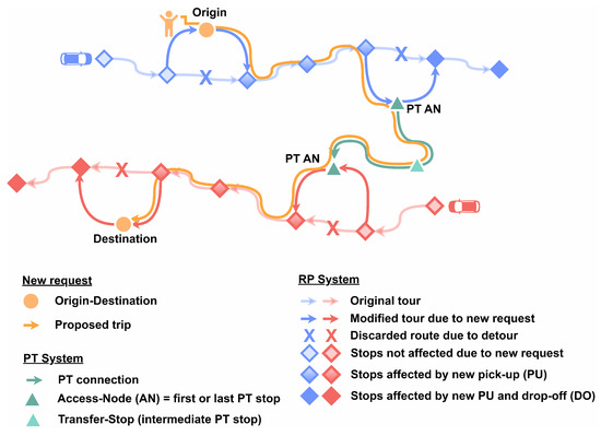
Figure 1.
Intermodal three-leg trip combining ride-pooling (blue and red legs) with public transportation (green leg). Source:created by the authors.
Figure 1.
Intermodal three-leg trip combining ride-pooling (blue and red legs) with public transportation (green leg). Source:created by the authors.

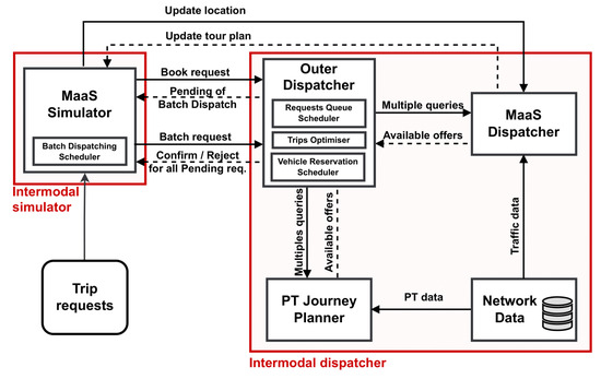
Figure 2.
Architecture of the intermodal system. Source: created by the authors.
Figure 2.
Architecture of the intermodal system. Source: created by the authors.
The intermodal simulator is a modified version of the MaaS simulator, which was originally designed for ride-pooling scenarios. It follows an event-scheduling approach in which two agents represent vehicles and customers. In the intermodal context, booking requests are handled by the intermodal dispatcher core, known as the outer dispatcher, while the ride-pooling fleet management requests are handled by the ride-pooling dispatcher, the so-called MaaS dispatcher. Within this simulator, journeys encompass up to three legs, with ride-pooling serving as a feeder for the transit network during the first and/or last legs. The preliminary version of this simulator was presented in [22].
The system employs a batch dispatching approach in which requests are grouped together and dispatched simultaneously to optimise the system’s resources, particularly those of the ride-pooling fleet. To manage requests that arrive early, it also incorporates a delayed-dispatch technique to handle the challenge of predicting the availability of suitable vehicles in cases when the entire timeframe for a tour is unoccupied. In the case of intermodal trips in which ride-pooling is the last leg (PT + RP and RP + PT + RP trips), the system dispatches the journey in two steps. Initially, the first part of the trip is dispatched according to an estimate of the remaining last leg, and the last leg is dispatched when its time window approaches. This approach considers new artificial requests—referred to here as last leg (LL) requests—which must be coordinated with the preceding public transport leg. This innovative dispatch methodology was first presented in [19].
The study by [19] focused on addressing fundamental operational policies, as mentioned in the introduction of this paper. Building upon the knowledge gained from these preliminary experiments, the authors recognise the need for further enhancements and have conducted additional computational experiments, which serve as the primary contribution of this present research. Our main objective here is to achieve the following:
- Fleet size: determine the optimal vehicle ratio necessary to efficiently handle requests within the system.
- Batch size: investigate the importance of batch size, taking into account queue lengths and considering computational issues.
- LL dispatch time advance: assess the impact of delaying the dispatch of last leg requests and evaluate different time advances or absences of delays.
- LL vehicle reservation time advance: monitor potential vehicles to serve last leg requests and evaluate different time advances for a vehicle reservation or assess the absence of vehicle reservations.
- Enable requests for multiple passengers sharing the same origin and destination, such as families, colleagues and so on.
Section 2 provides a summary of the approach adopted to address the issues described above. Section 3 presents the model enhancements. Section 4 outlines the full parametrisation of the system. The computational experiments are described in Section 5, and the results of those experiments are analysed in Section 6. Finally, the research findings are discussed in Section 7, where conclusions are drawn and potential future lines of research are identified.
2. Summary Description of the Approach Taken
For a more comprehensive understanding of the objectives and model enhancements discussed in this paper, detailed descriptions of the approach components can be found in [19]. To provide clarity and context, a summary description of the objectives and model enhancements relevant to this paper is included.
2.1. The Intermodal Simulator
The intermodal simulator is designed to emulate real-world scenarios and evaluate the case study by advancing simulation time, updating road network estimates and calculating relevant KPIs for scenario analysis. It uses an event-scheduling approach with a time-sorted event queue and two agents: vehicles and customers. These agents generate events that modify their states during the course of the trip.
2.1.1. Vehicle Agent
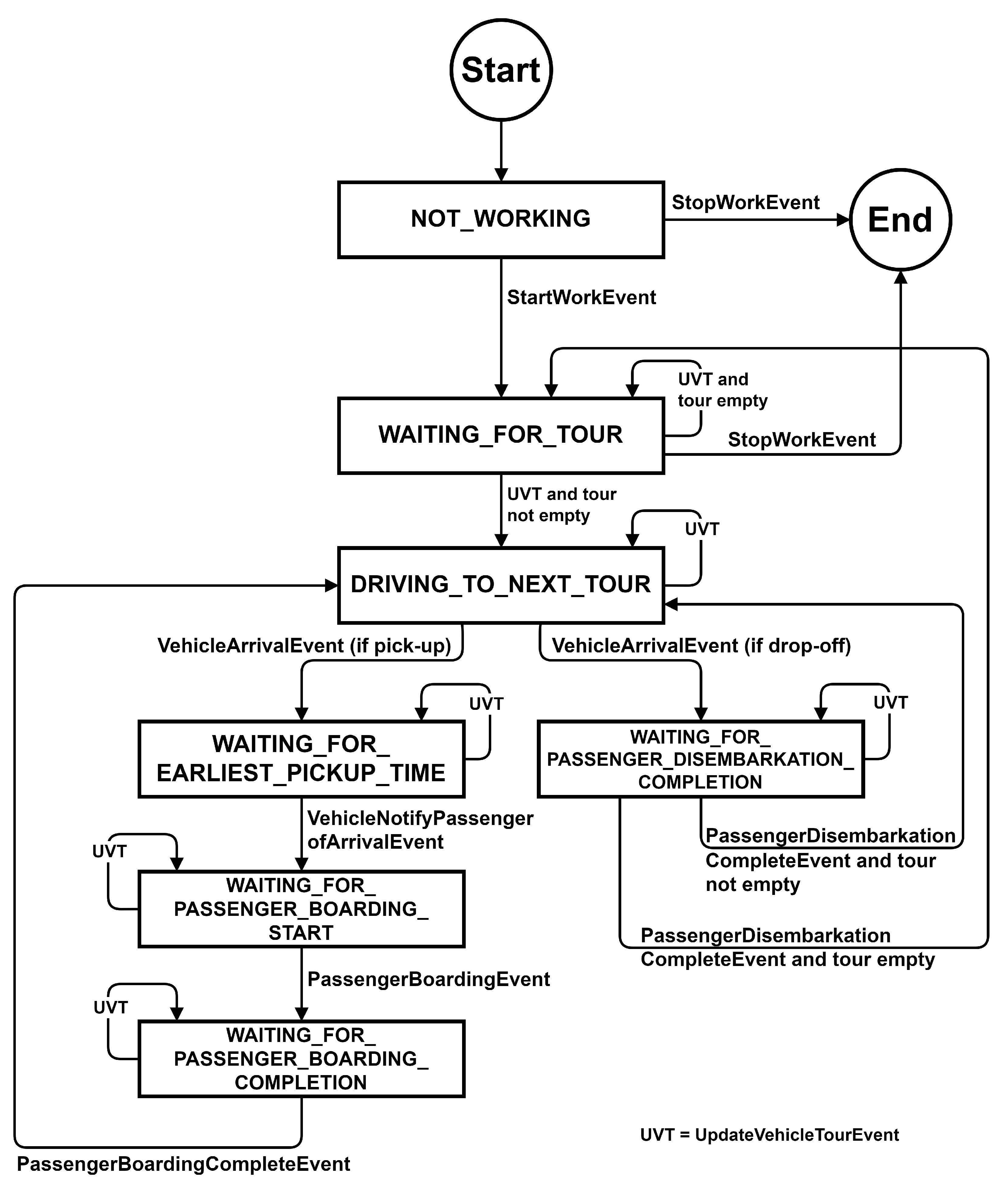
As depicted in the diagram in Figure 3, the states of the vehicle agents correspond to different stages of the vehicle’s journey, such as driving to the next point in the route, waiting at pick-up (PU) locations, waiting for passenger boarding to complete and completing a drop-off (DO) at a passenger’s destination. The intermodal approach does not impact the states of the vehicle agents, as each ride-pooling leg is treated as a separate request.
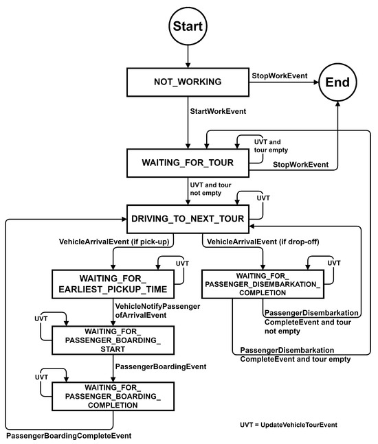
Figure 3.
Vehicle agent states. Source: created by the authors.
2.1.2. Customer Agent
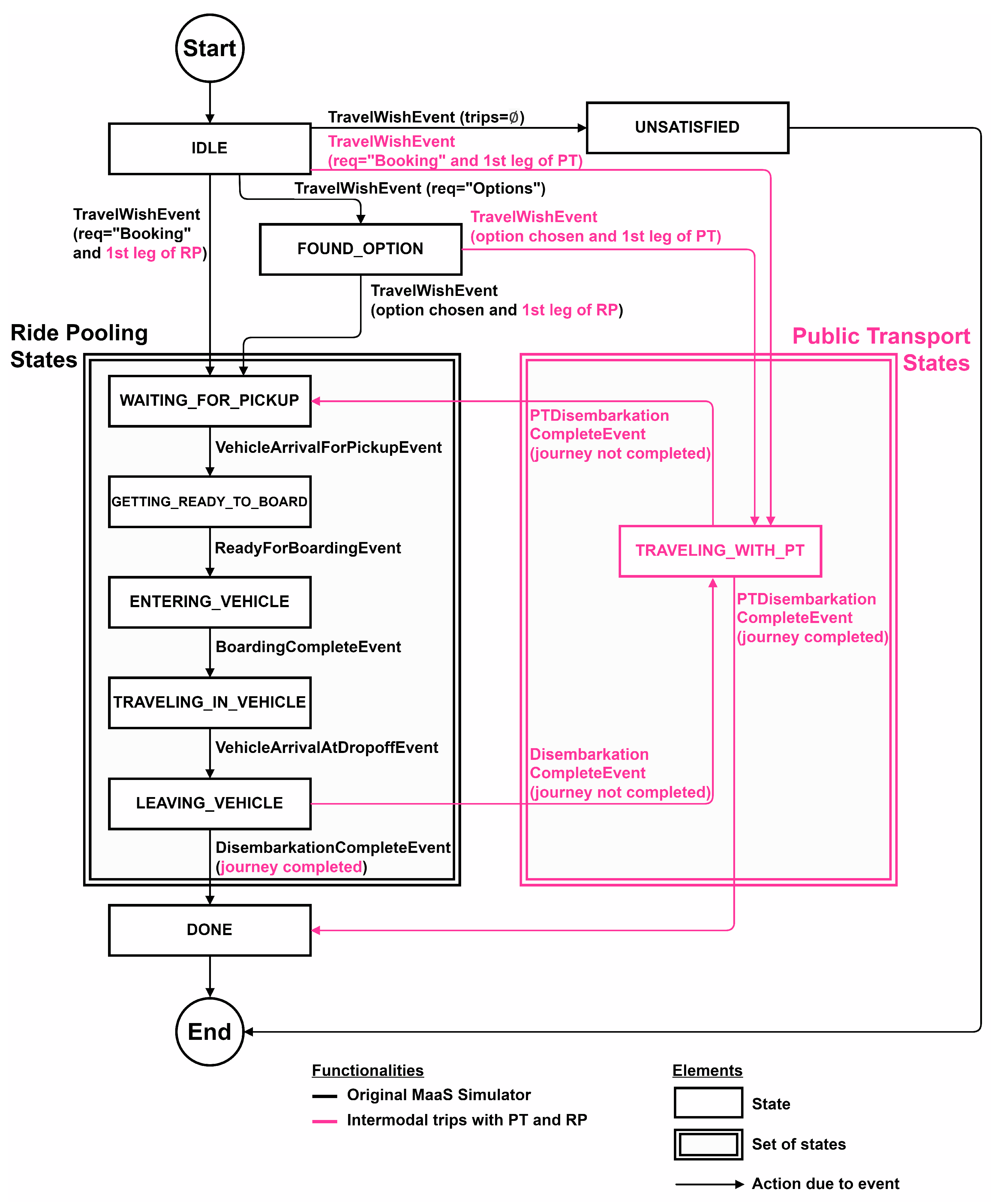
The customer agent manages the operations related to booking requests. In the original ride-pooling scenario depicted in black on the left-hand side of Figure 4, the customer could only take a ride-pooling-exclusive trip by transitioning through the corresponding states: WAITING-FOR-PICKUP, GETTING-READY-TO-BOARD, ENTERING-VEHICLE, TRAVELLING-IN-VEHICLE, LEAVING-VEHICLE and DONE. If no feasible trip is found, the customer agent transitions to the UNSATISFIED state.
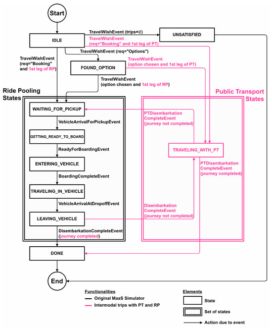
Figure 4.
Intermodal trips in customer agent states (pink shows modifications). Source: created by the authors.
In the intermodal scenario, customers have the option to book trips with up to three legs. The revised states are depicted in pink on the right-hand side of Figure 4. If the trip starts with a ride-pooling leg, customers transition to WAITING-FOR-PICKUP. On the other hand, if the trip starts with public transport, customers transition to a new state called TRAVELLING-WITH-PT. Including transfers allows customers to switch to the other transport mode when a leg is completed, utilising the “Disembarkation-Complete” event for RP and “PT-Disembarkation-Complete” event for PT. Finally, customers transition to the DONE state when the entire trip is completed.
In the batch dispatching approach, which is depicted in blue at the top of Figure 5, customers enter a PENDING state and wait for a batch response that resolves all of the requests in the queue. If a tour plan is provided, the simulation proceeds normally. Otherwise, customers may be offered another attempt to find a suitable solution. If no attempts remain, then the customer is ultimately rejected.
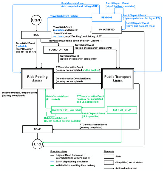
Figure 5.
Batch dispatching and correction for three-leg trips in customer agent states (blue and green are modifications). Source: created by the authors.
In situations where customers have already left the PT system but are still waiting for their last leg dispatch (PT + RP and three-leg trips), a WAITING-FOR-LAST-LEG state is introduced. This state is depicted in green at the bottom of Figure 5. If the system successfully books a ride-pooling vehicle, the customer proceeds as usual. If the system is unable to serve the customer, the agent remains in that state or transitions to a new state called LEFT-AT-STOP.
2.2. Enhanced Optimisation Model for Intermodal Dispatching
The information flow illustrated in Figure 2 depicts the interaction between the outer dispatcher, the MaaS dispatcher and the PT journey planner to determine intermodal tour plans for a group of requests. The procedure has been extended to include multiple-passenger requests and now comprises three steps: a candidate search method to identify suitable candidates, estimation of potential combinations that consider time restrictions and vehicle availability, and the use of an optimisation model to determine optimal assignment.
2.2.1. Step 1: Candidate Search Method
A filtering procedure identifies suitable interchange points. First, the search space is limited to a specific radius, and the transport mode is determined based on distances to the stops. Stops within a certain close distance are assumed to be reachable on foot, while those farther away are determined to require the use of ride-pooling. Estimated travel times are then used to select the most favourable candidates.
2.2.2. Step 2: Potential Intermodal Trip Determination
The PT journey planner and the MaaS dispatcher are utilised to identify suitable combinations of ride-pooling (RP) and public transport (PT) legs. The expected pick-up/drop-off (PUDO) times of RP vehicles are determined by taking the RP fleet’s congestion during the specific time window into account. Departure choices from an origin stop to a set of destination stops are made based on the concrete arrivals and departures listed on the public transportation system’s timetable.
The intermodal fare system takes into account the fare for each leg: using a single-ticket fare for a PT leg and a modified version of the fare system proposed by [24] for an RP leg. The modified system is summarised below in Formula (1), which assumes a regular taxi fare per kilometre, denoted as p. The distance travelled individually () is fully paid, while the distance shared with other passengers (, shared with m passengers) is evenly split, with a small inflation parameter . Additionally, a base fare b is included to reflect the functioning of shared services in practice. This formula imposes no minimum fee for the RP leg, as it is generally shorter in an intermodal scenario compared to an exclusive ride-pooling scenario.
To account for multiple-passenger requests, Formula (1) has been modified from the version presented in [19]. The formula expresses the amount to be paid for all r passengers in the request while also taking the common distance travelled together into account.
2.2.3. Step 3: Optimal Modal Trip Composition (OMTC) Module
The OMTC module uses an optimisation model to assign requests to candidate PT transit stops and RP vehicles. The model determines the modal composition of the trip requests based on the availability and capacity of RP vehicles and suitable PT-AN locations. Various factors are taken into account, such as the type of requests (here and now, placed at that instant; booking requests, placed in advance; or last leg requests, coming from an already initiated trip). Other factors include priority levels and the user’s intermodal preferences (requesting an RP-exclusive trip, PT included, or no preference). The model assumes a set of requests, a set of vehicles and a set of PT stops. Null-taxi and null-stop are used to represent trips that do not use the RP or PT system.
The graph in Figure 6 illustrates the decision-making process for each client. Blue arrows represent RP-exclusive trips, where an RP vehicle is assigned but no PT stop is involved. This also applies to the last leg of already initiated trips (PT + RP and RP + PT + RP). The pink arrows represent RP + PT and RP + PT + RP trips, where both an RP vehicle and a PT stop are assigned. In the case of RP + PT + RP trips, the estimated cost of the trip includes an estimation of the last leg, which will be dispatched in a subsequent iteration, if selected. Green arrows indicate PT-exclusive and PT + RP trips, with the latter also including an estimation of the last leg. Finally, black arrows represent customers who are not served.
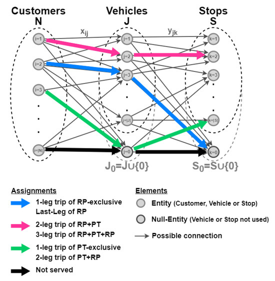
Figure 6.
Diagram of relationships between customers, vehicles and stops. Source: created by the authors.
The mathematical model presented in [19] calculates the trajectories for each request depicted in Figure 6. This is accomplished by incorporating cost coefficients based on trip travel times and user fares as well as a set of priorities based on the types of requests. Penalty terms are also included to enforce these priorities. The solutions provided by the model aim to satisfy both the system operator and the user. To account for multiple-passenger requests, the model has been extended with a new constraint, denoted as Equation (2). This constraint can be described as follows: if a request i is assigned to a vehicle j (), then the sum of the number of passengers in request and the passengers already onboard the vehicle cannot exceed the capacity of the vehicle, denoted as c.
3. Enhancements to the Approach
To enhance the accuracy and performance of the previous methodology and achieve better research outcomes, we have made the following improvements:
- Modification of the MaaS dispatcher to enable booking the specific ride-pooling legs determined by the optimisation model included in the outer dispatcher. This extension was then integrated into the intermodal system. Now, the booking is first requested to the MaaS dispatcher. If the dispatched vehicle does not align with the vehicle assigned by the outer dispatcher, the dispatched tour plan is discarded and the desired tour plan is substituted instead.
- Modification of the outer dispatcher for multi-passenger requests. This entailed the following two tasks:
- –
- Defining a new fare system, as described in Section 2.2.2.
- –
- Modifying the basic optimisation model to accommodate seat availability, as described in Section 2.2.3.
- Full parametrisation of the system: to enrich and facilitate the definition of scenarios and computational experiments, we converted the model into a virtual lab to test designs and policies.
4. Full Parametrisation of the System
The simulation-based intermodal system presented here was meticulously designed and incorporates numerous parameters that simplify the definition of scenarios and computational experiments. These parameters can be categorised into three main groups: those related to the scenario, quality of service, and system performance. The specific parameters are:
- Intermodal system configuration
- –
- Candidate search (first step in the dispatching algorithm):
- ∗
- Search areas to determine walkable access and RP access: These define the two search areas for transit stops and are directly related to the scenario being considered.
- –
- Potential intermodal trips (second step in the dispatching algorithm):
- ∗
- Fare system: This comprises the base fare b, fare per km p and fare inflation . The first two are scenario-related, while fare inflation is set to 0.5, as in [24,25].
- ∗
- Best number of vehicles for an LL estimate: This parameter helps to estimate waiting times for vehicle arrivals and travel times to destinations at stops. This parameter is related to the quality of service.
- –
- Optimal trip composition (third step in the dispatching algorithm):
- ∗
- Fare and time weights in the cost function: This accounts for the desirability of the fare and time with regard to trip assignments, represented using and , respectively. This parameter is related to both the scenario and quality of service.
- –
- Hybrid batch dispatching configuration
- ∗
- Batch frequency: This parameter is related to the quality of service and system performance and has a value set to 30 s, as used by [26,27].
- ∗
- Batch size: This parameter helps to protect the system during peak periods by processing the batch of pending requests once a specific number of requests is queued. This parameter is related to system performance.
- –
- Last leg configuration (LLC): This parameter configures the delayed last leg dispatching strategy. It is related to the quality of service:
- ∗
- Delayed LL dispatching time advance.
- ∗
- Vehicle reservation for LL availability time advance.
- Ride-pooling service configuration: This accounts for the fleet size and seat capacity c. This parameter is related to the quality of service.
- Demand profile: This accounts for input demand according to three essential factors:
- –
- Request type: Here-and-now (HN) requests (placed immediately) and booking (B) requests (placed in advance (assumed 30 min)).
- –
- Intermodal preference: This parameter indicates the preference for different modes. Pure-RP (a) identifies exclusively ride-pooling trips. PT (b) is included for trips that include public transport. Indifferent (=) indicates no preference.
- –
- Number of passengers per request: This parameter ranges from single-passenger requests (1) to the vehicle’s seating capacity (c) for multi-passenger requests.
The first two parameters were introduced with the new dispatching methodology presented in [19]. The latter parameter, the number of passengers, is a new addition that is required to analyse multi-passenger demand.
5. Addressing the Open Questions
The complexity of fully parameterising the system leads to a combinatorial explosion of scenarios when exploring numerous values for each parameter. To manage this, we have reduced the system to a computationally manageable number of alternatives for the most relevant factors. The chosen values, which are expected to significantly impact the system’s performance, are as follows:
- Intermodal system configuration:
- –
- Batch size: We assess different batch size limits of 1, 10 and 30 requests. A batch size of 1 dispatches the request immediately upon receipt, while larger batch sizes dispatch accumulated requests either when the limit is reached or every 30 s (hybrid batch dispatching).
- –
- LL configuration (LLC): We evaluate five different setups:
- LL dispatch not delayed (vehicle reservation not required);
- LL dispatch time advance of 40 min without vehicle reservation;
- LL dispatch time advance of 30 min without vehicle reservation;
- LL dispatch time advance of 40 min with vehicle reservation 60 min in advance;
- LL dispatch time advance of 30 min with vehicle reservation 60 min in advance.
- Ride-pooling service configuration: We explore various fleet sizes of 100, 200, 300 and 400 vehicles.
- Demand profile: We evaluate two different demand profiles:
- All requests consist of a single passenger.
- Requests consist of 77% single-passenger rides, 17% two-passenger rides, 4% three-passenger rides and 2% four-passenger rides. These realistic proportions have been obtained from published reports on yellow taxi fleet usage in New York City [28], as no information was available for the experimental area described below.
This experimental design comprises a total of 60 configurations for each demand profile, resulting in a total of 120 experiments.
The research focuses on the inner region of the metropolitan area of Barcelona, Spain. Information was obtained from the Virtual Mobility Lab network model, which incorporates all public and private transport modes, as presented in [29]. The study area, referred to as the test area (TA), is shown in Figure 7 and encompasses multiple municipalities. The transit network comprises the Integrated System of Metropolitan Mobility of Barcelona (SIMMB), which includes bus, metro, tram, rapid transit systems and commuter railways. It encompasses approximately 3000 stops, 300 distinct lines and over 6000 services during the operational horizon assumed in the tests. The private traffic network is composed of 114,000 links and 87,300 nodes.
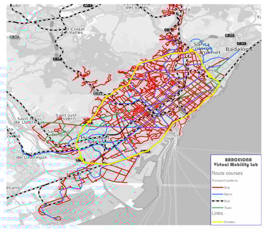
Figure 7.
Test area and its diverse modes of public transportation. Source: created by the authors with PTV Visum’s software, full version 2022 (academic license).
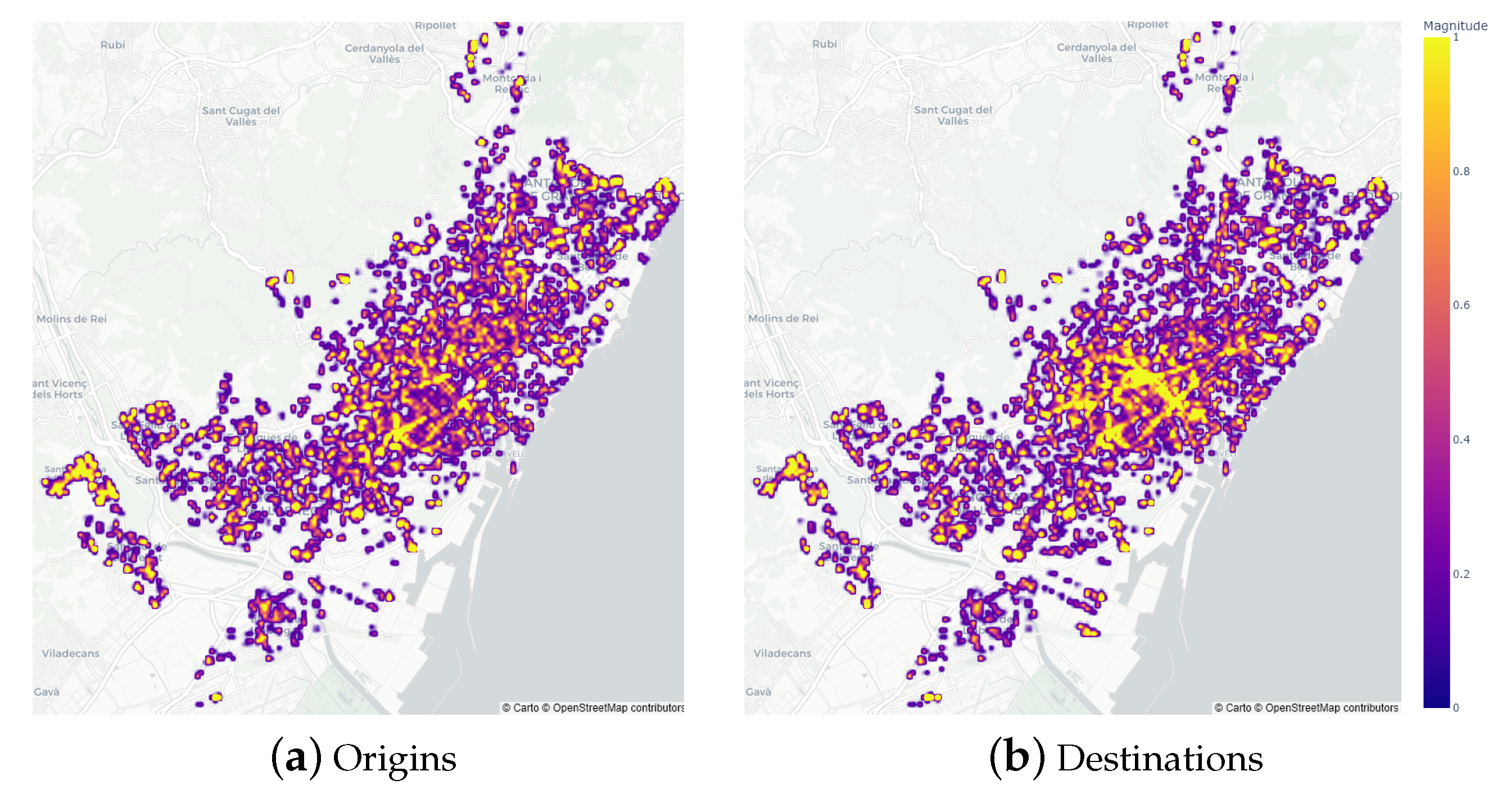
To analyse mobility patterns between the origin and destination areas of the demand, the TA was divided into two subareas: the IN area, which is within Barcelona’s Rondes, the city’s high-capacity belt road, and the OUT area, which is situated outside the belt road. The demand utilised consists of 10,031 trip requests spread over a 4-h period, with the request origins and destinations shown in Figure 8. This demand generation accounts for various factors of the global transport demand in the test area, which was calibrated using information collected from mobile operators and historical data published by the area’s transport authorities, as described in [29]. As depicted in the origin and destination maps, most morning commutes originate from various locations across the area but are primarily directed towards the city centre, where the majority of businesses and entertainment venues are situated. It is assumed that the majority (80%) of requests are immediate requests and that only 20% are bookings made 30 min in advance of travel. We additionally assume an intermodal preference distribution of 65% indifferent, 30% with integrated PT and only 5% as RP-exclusive. The demand is assumed to be distributed uniformly between the various groups considered.

Figure 8.
Volume of requests according to origin and destination locations. Source: created by the authors using the Plotly Express graphing library.
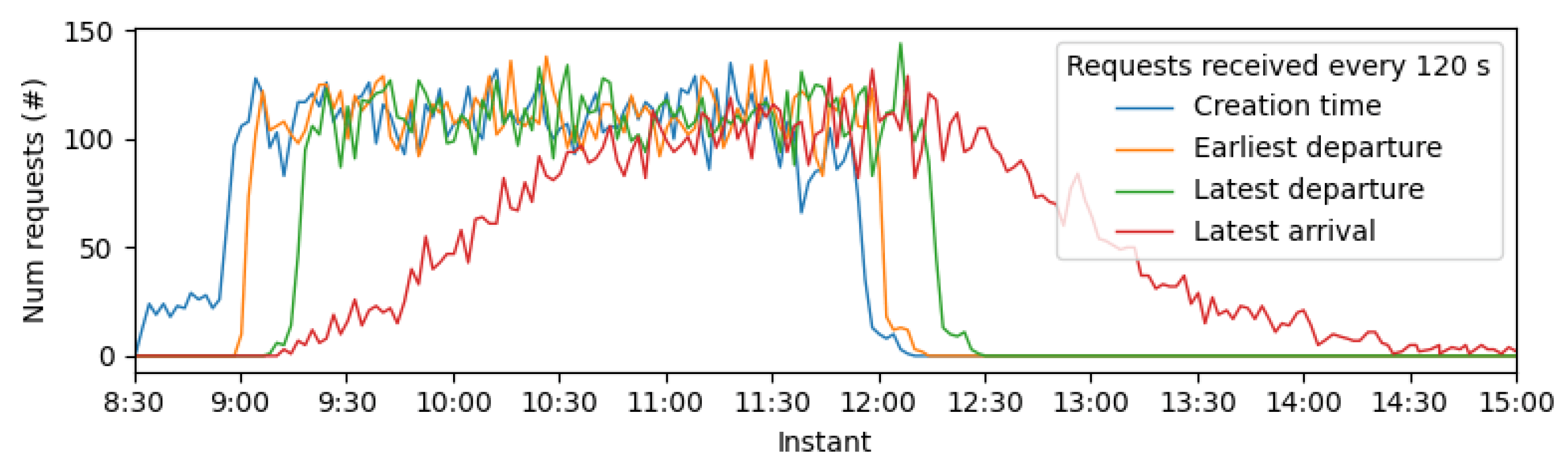
The generation rate of the requests, along with their earliest and latest departure times, is depicted in Figure 9. The requests are assumed to arrive continuously from 9 a.m. to noon at a rate of approximately 55 requests per minute. However, the latest arrival time for each request varies and is determined based on the distance between the origin and destination. The gap between 8:30 and 9 a.m. between the creation and earliest departure is due to the reception of booking requests, which arrive 30 min in advance.
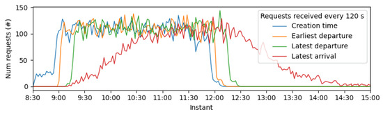
Figure 9.
Distribution over the simulation period for creation, earliest departure, latest departure and latest arrival times for the generated requests. Source: created by the authors.
6. Results Analysis
6.1. Demand Profile 1: All Single-Passenger Requests
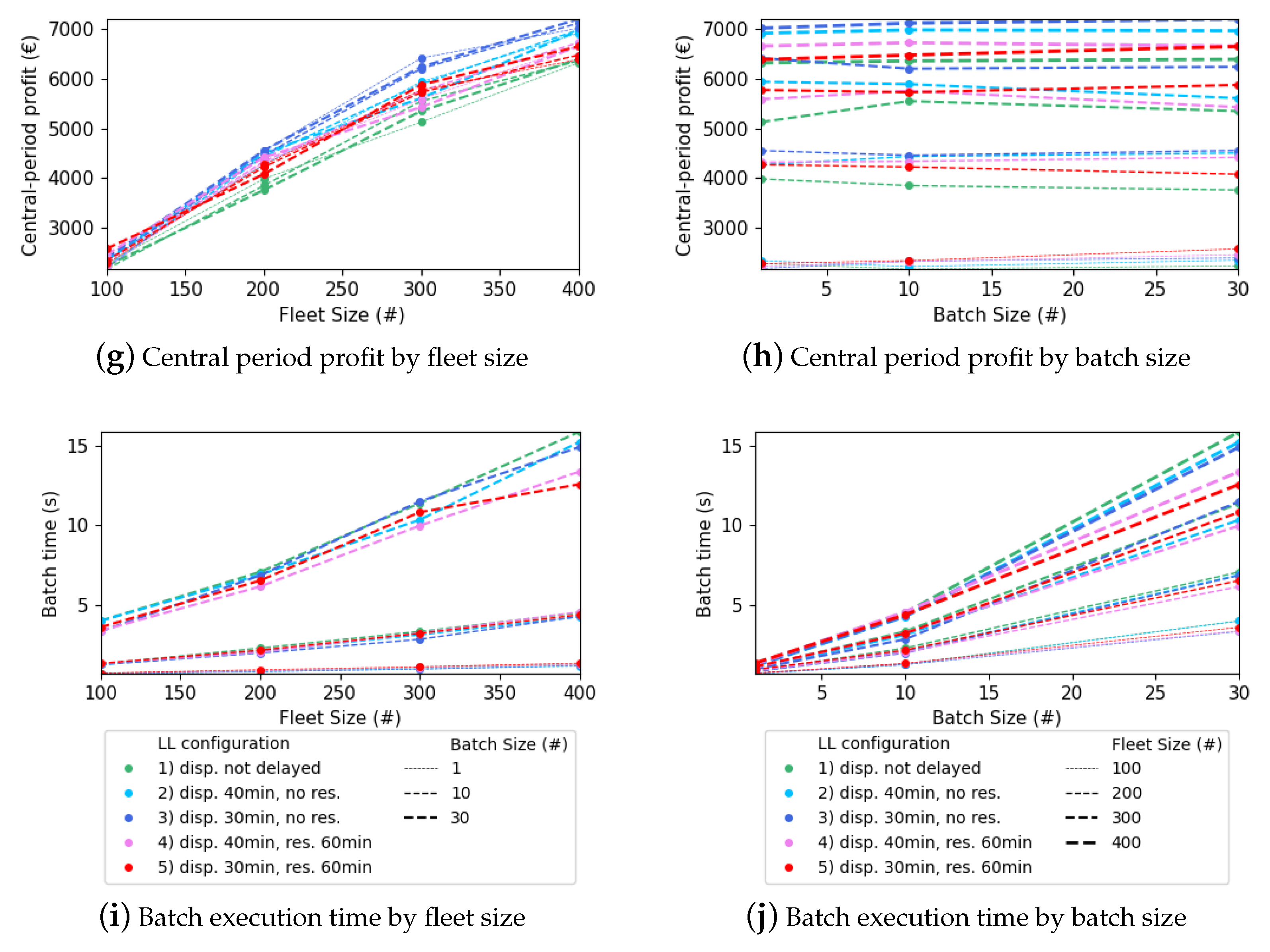
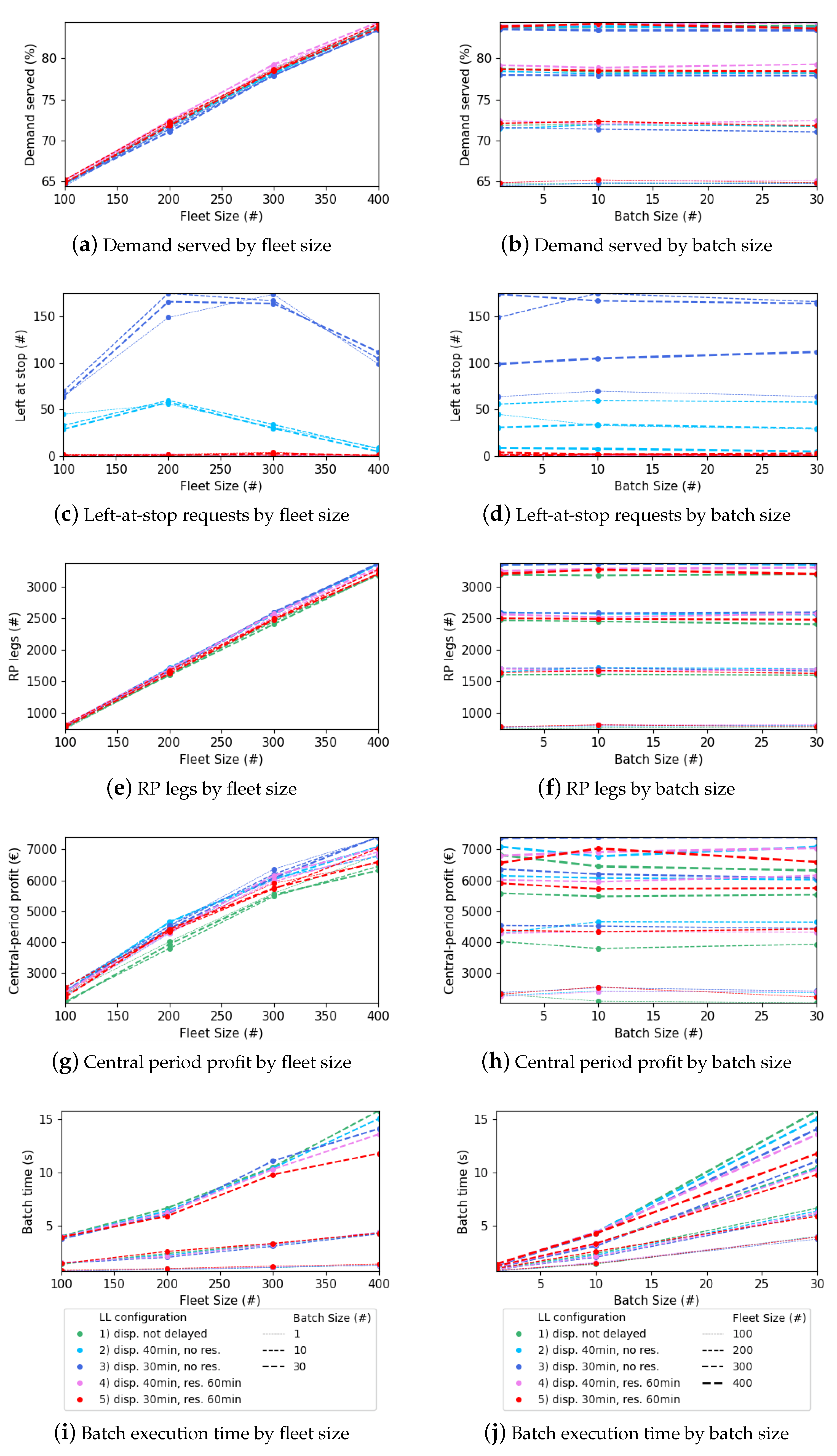
Several key performance indicators (KPIs) are used to evaluate the impact of each tested configuration. These KPIs include the service demand, uncompleted requests (left-at-stop), ride-pooling legs served, central period profit and batch execution time. Figure 10 shows the results of our analysis of these KPIs according to fleet size (left) and batch size (right). Different line widths distinguish batch sizes (left) and fleet sizes (right), while colours represent LL configurations. Based on this preliminary analysis, four aspects stand out:
- Batch size: The batch size has a significant impact on system performance. When the batch size is too small (e.g., one request), the execution times increase significantly. Grouping requests through batch dispatching allows for parallelisation of the dispatching algorithm: distributing calculations and reducing execution times. However, the batch size must be chosen carefully, as larger limits (30 requests in our design) increase the size of the optimisation model. An intermediate limit (10 requests) yields better time-performance outcomes without compromising the quality of the solution. The service demand only demonstrates minor fluctuations in the central period profit.
- Fleet size: Fleet size greatly impacts the service demand. Small fleets (100–200 vehicles) can service fewer requests, leading to an increase in the number of left-at-stop requests as the fleet becomes saturated. On the other hand, the number of ride-pooling legs served increases linearly with the fleet size, as the presence of more vehicles enables additional trips and RP legs to be completed. This, in turn, leads to an increase in the central period profit and system performance.
- LL dispatch delay: All LL configurations achieve similar levels of service demand. However, in configuration LLC1, the system is utilised less efficiently, resulting in lower profits. When an LL is dispatched, most vehicle tours during that time window are empty, thus constraining the dispatching of future requests.
- Vehicle reservation: This strategy has a significant effect on the number of left-at-stop requests when LL dispatch is delayed, nearly eliminating them all and increasing profits. Consequently, vehicle reservation outperforms configuration LLC1.
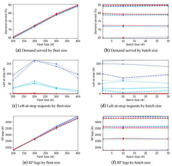
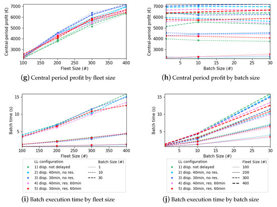
Figure 10.
Demand profile 1: analysis of demand served, left-at-stop requests, ride-pooling legs dispatched, central period profit and batch execution time according to fleet size and batch size. Source: created by the authors.
Figure 10.
Demand profile 1: analysis of demand served, left-at-stop requests, ride-pooling legs dispatched, central period profit and batch execution time according to fleet size and batch size. Source: created by the authors.
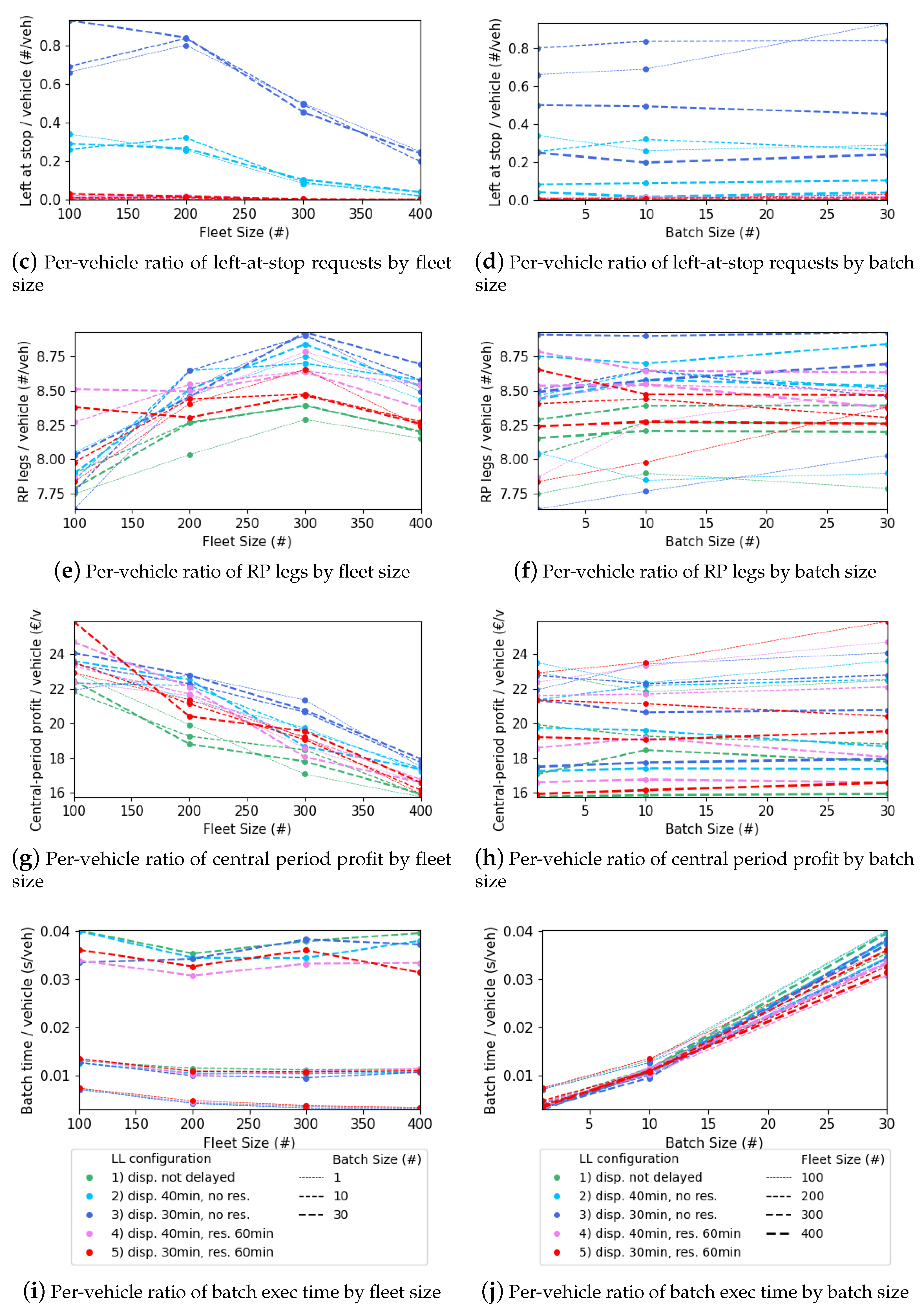
The analysis of these KPIs with respect to the fleet size reveals additional effects, as depicted in Figure 11.
- The number of served ride-pooling legs shows a linear increase with the fleet size. However, with a fleet of 400 vehicles, the number of served ride-pooling legs decreases slightly, which is unexpected considering the presence of unserved requests (around 20%, as shown in Figure 10). Moreover, configuration LLC1 clearly dispatches fewer ride-pooling legs compared to the other configurations, as indicated by the green lines consistently remaining below those of the other configurations.
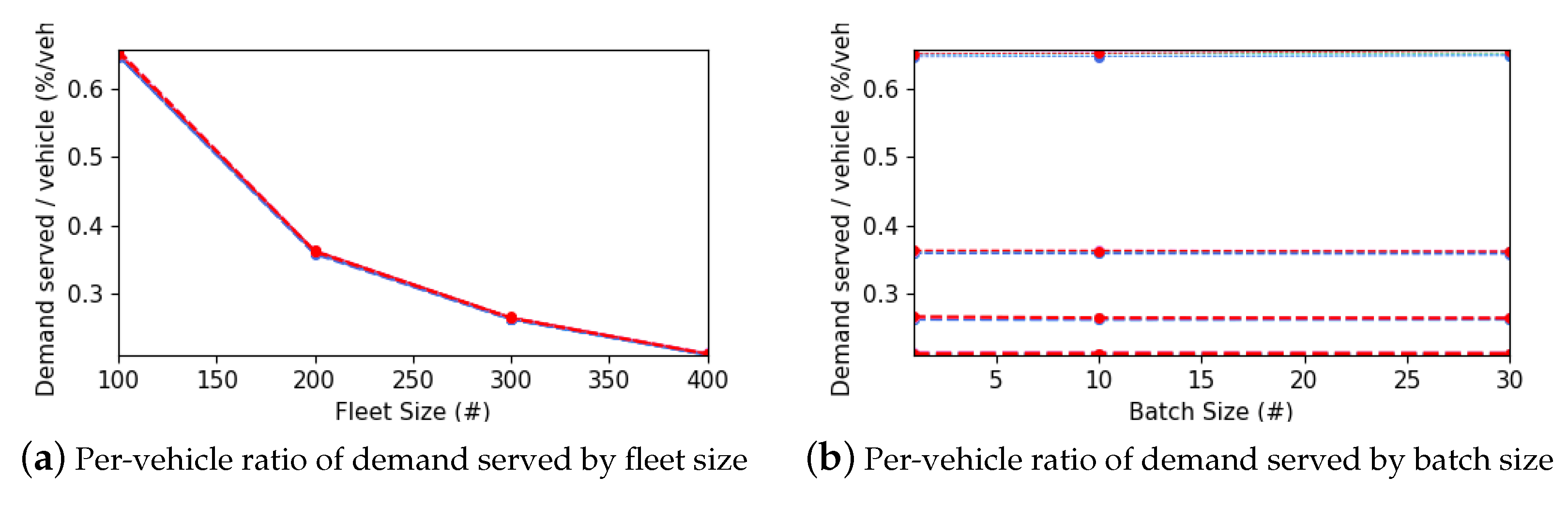
- The ratio of the service demand per vehicle decreases as the fleet size increases. This decline is accompanied by a reduction in the ratio of central period profit per vehicle since the increase in the service demand is insufficient to cover all the operational costs of the fleet. Moreover, configuration LLC1 notably achieves the lowest profits.
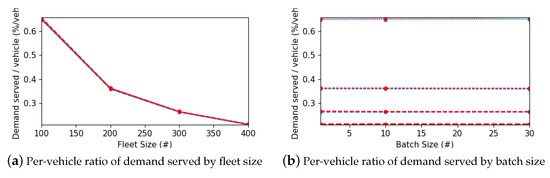
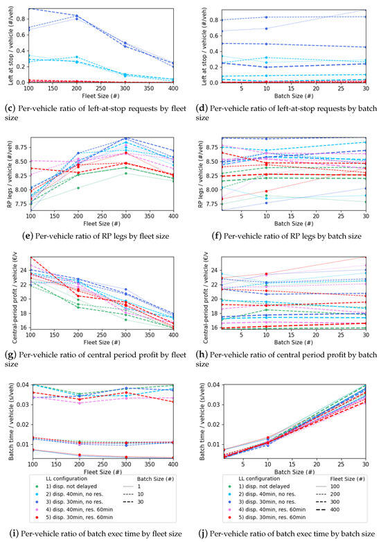
Figure 11.
Demand profile 1: analysis of the per-vehicle ratio of demand served, left-at-stop requests, ride-pooling legs dispatched, central period profit and batch execution time according to fleet size and batch size. Source: created by the authors.
Figure 11.
Demand profile 1: analysis of the per-vehicle ratio of demand served, left-at-stop requests, ride-pooling legs dispatched, central period profit and batch execution time according to fleet size and batch size. Source: created by the authors.
6.1.1. Performance Analysis of the Most Efficient Configurations
Based on the initial findings, the use of an intermediate batch size of 10 requests is recommended rather than 1 or 30. This choice offers similar outcomes but improves time performance. Configuration LLC3 is discarded due to its poor performance in handling left-at-stop requests. Furthermore, a fleet size of 400 vehicles is selected for further assessment, as it is able to achieve higher demand satisfaction and profitability while reducing travel time compared to smaller fleet sizes.
Among the four remaining LL configurations (LLC1, LLC2, LLC4 and LLC5), all yield similar results in terms of the service demand, with an average of approximately 8500 requests satisfied. The distribution across intermodal types is also similar, with an average of 1500 RP-exclusive trips, 5300 PT-exclusive trips, 660 RP + PT trips, 800 PT + RP trips and 190 three-leg trips.
The travel times, distances and fares for each intermodal trip type are comparable across all LL configurations. Therefore, Table 2 and Table 3 only present these KPIs for LLC4. The “Direct” row reports the travel time, distance and fare for a customer travelling in a private vehicle. The “Expected” row reports the system’s initial estimate, while the “Actual” row shows the outcome experienced after factoring in all future detours. PT trips have the shortest travel times, followed by RP and RP + PT trips, PT + RP trips and three-leg journeys. Although one might expect RP + PT and PT + RP trips to have similar travel times and distances, this is not the case. RP + PT trips allocate a smaller margin for detours in the RP leg to ensure the scheduled PT departure is not missed. In contrast, PT + RP trips allow more detours, as RP occurs at the end of the trip. Moreover, waiting times for the last ride-pooling leg are shorter in PT + RP trips since the vehicle is prescheduled to arrive on time. Regarding fares, it is evident how users transitioning from a private vehicle to PT or from an intermodal option experience significant reductions in fares. In this case, direct fares correspond to the direct costs of gasoline for private vehicles; however, this does not encompass the subsequent costs related to car ownership (purchase, maintenance and insurance) or the price of a parking spot at the destination. The expected and actual fares consider the combined fares for all legs, where the RP fare is based on the distance travelled and includes discounts if the vehicle is shared with other passengers (as per Formula (1)), and the PT fare accounts for the single-ticket cost.
Table 2.
Demand profile 1, 400V_10R experiments: summary of mean travel times for each intermodal type.
Table 3.
Demand profile 1, 400V_10R experiments: summary of mean distances and fares for each intermodal type.
Table 4 summarises the time delays during system decisions for each request type (HN, B and all combined) and for each kind of trip. This analysis focuses on configurations LLC1, LLC2 and LLC4 to show the most distinct scenarios (LL not delayed, LL delayed without reservation and LL delayed with reservation). The system quickly identifies whether or not a request can be serviced in the next batch, reducing the time customers wait for a response from the system. In LLC1, all LL requests are dispatched during the next batch. However, in the delayed configurations, the delay can range from 8 to 11 min for HN and from 20 to 23 min for B requests. Notably, LLC2 left seven customers waiting at a stop for an average of 38 min, indicating that these requests could have been discarded during a previous iteration to avoid wasting system resources.
Table 4.
Demand profile 1, 400V_10R experiments: summary of time delays during system decisions.
The profit analysis shown in Table 5 evaluates the RP system’s revenue from fares, driver salaries and fuel costs. Over the total period of 6.5 h, no configuration appears to be profitable. However, the warm-up and cool-down periods, each lasting 1 h, significantly affect the results. These periods represent a large portion of the total time, during which few requests are served but the full fleet of drivers remains active, leading to considerable losses. However, if the analysis is focused on the 3.5-h central period when the system is fully operational, the system appears to indeed be profitable. This period better reflects the characteristics of a full day’s operation, where the impact of warm-up and cool-down periods is minimised. Nevertheless, all of the LL configurations prove to be profitable, with the greatest profitability observed when LL is delayed, as this optimises the system resources more efficiently.
Table 5.
Demand profile 1, 400V_10R experiments: profit analysis for the 6.5-h total period (from 8:30 a.m. to 3 p.m.) and the 3.5-h central period (without warm-up and cool-down periods, from 9:30 a.m. to 1 p.m.).
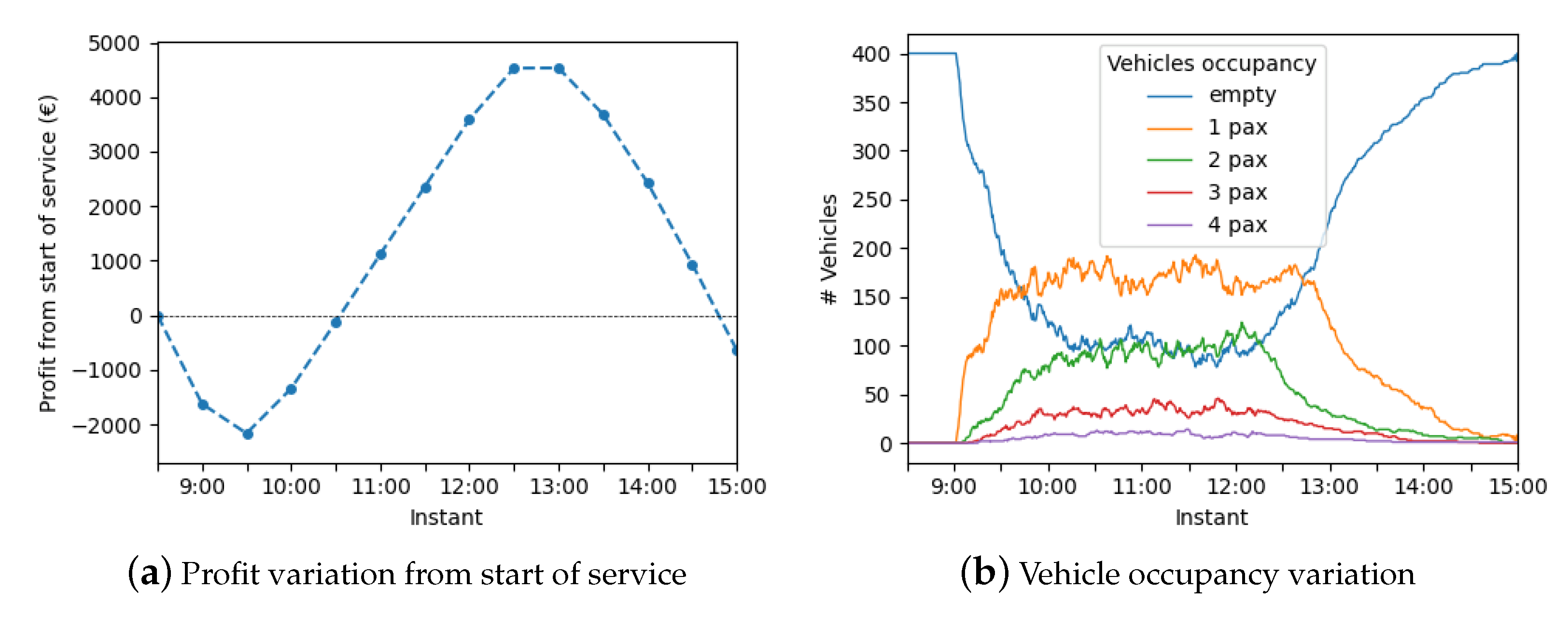
To highlight the changes in profitability over the total period, Figure 12 depicts the cumulative profit from the beginning of service on the left and the fluctuations in ride-pooling vehicle occupancy (directly linked to profit) on the right. As these results are comparable across all LL configurations, only the results for LLC4 are shown. The graph clearly demonstrates an increase in profit during the central period but decreases during the warm-up and cool-down periods. During our experiments, all of the drivers’ salaries were maintained over the course of the total period. Despite this, the system remains profitable for all LLs of the studied configurations, with better profitability being observed when LLs are delayed. Remarkably, the four-seat capacity used for the fleet of vehicles is not a limiting factor since very few vehicles carry four passengers at a time.
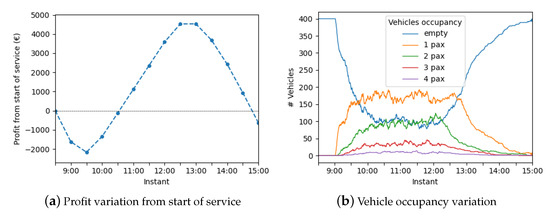
Figure 12.
Demand profile 1, 400V_10R_LLC4 experiment: comparison of the variation in profit with vehicle occupancy. Source: created by the authors.
The results indicate that the system consistently performs well across all of the studied LL configurations, with a batch frequency of 10.2 s to 11.5 s and an average execution time of 3.1 s per batch.
6.1.2. PT Network Utilisation Analysis
To gain further insights into the effects of combining ride-pooling and public transport on the use of the PT system and mobility patterns in the test area, the following analysis focuses on LLC4, and the results obtained are comparable across all of the studied LL configurations.
Figure 13 illustrates the access nodes used by the dispatched requests. It reveals that most of the stops are located along major roads in Barcelona, while in the periphery, where the transfer options are limited, stops are concentrated at only a few locations.
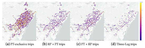
Figure 13.
Demand profile 1, 400V_10R_LLC4 experiment: volume of access nodes used. Source: created by the authors using the Plotly Express graphing library.
Table 6 provides a detailed analysis of PT usage, categorised by intermodal type. The table presents the number of trips made using each transit mode, specifying whether the PT leg includes a transfer or if only a single line was used. It also includes data on the proportion of trips in each category and the average transfer time, calculated as the interval between the arrival of the first transit mode and the departure of the next. The data indicate that most trips rely on a single transit line, with very few transfers occurring between lines, possibly due to long waiting times and the additional walking required. Intermodal trips that include a ride-pooling leg also incur waiting times at access nodes, making internal PT transfers less appealing. This also explains why the average transfer times during PT legs are relatively short; only options with stops that are situated close to one another and that can be reached quickly are appealing to users, as they do not cause significant idle times. The most popular transit modes for PT trips are the bus and subway systems, accounting for 82.3% of PT usage. However, as trips become longer, the usage of rapid transit modes increases, with train usage reaching 40.7% during three-leg trips, compared to only 14% in PT trips and 25% in two-leg trips.
Table 6.
Demand profile 1, 400V_10R_LLC4 experiment: analysis of transfers between principal transit modes used in dispatched PT legs.
To analyse mobility patterns, we divided the test area into two zones: the IN area and the OUT area. Table 7, Table 8 and Table 9 present the travel times, distances and fares for each trip type, which are categorised according to the IN and OUT areas containing the origin and destination points. The tables give the direct values (when using a private vehicle), expected values (when initially dispatched by the system) and actual values (after detours). The analysis shows that switching to the intermodal scenario significantly improves travel times for most types of trips (PT, two-leg and three-leg). The greatest reduction in travel time is observed for trips from the OUT area to the IN area, with a decrease of over 20 min. Fares for intermodal trips are also reduced to less than half of the costs associated with private vehicles, especially for trips starting and ending in the OUT area. However, RP trips do not result in reduced travel times compared to private vehicle options. Nevertheless, the service could still be competitive due to similar or slightly lower fares and the convenience of not having to drive or search for parking at the destination point.
Table 7.
Demand profile 1, 400V_10R_LLC4 experiment: distribution of travel times based on origin and destination points.
Table 8.
Demand profile 1, 400V_10R_LLC4 experiment: distribution of distances based on origin and destination points.
Table 9.
Demand profile 1, 400V_10R_LLC4 experiment: fare distribution based on origin and destination points.
Table 10 presents an overview of the service rates based on origin and destination points, intermodal preference and request type. Booking requests demonstrate a high service rate: exceeding 90% in most areas and for most preferences. However, accommodating trips with a preference of “Including PT” in the OUT–OUT area is more challenging, potentially due to limitations in the PT network. In such cases, an “RP” preference achieves a 100% service rate, proving that the proposed ride-pooling system may complement the transit network.
Table 10.
Demand profile 1, 400V_10R_LLC4 experiment: service rates based on origin and destination points, intermodal preference and request type.
6.2. Demand Profile 2: 77% Single-Passenger, 17% Two-Passenger, 4% Three-Passengers and 2% Four-Passenger Rides
The below analysis examines a multiple-passenger demand profile with up to four passengers per request. The objective is to assess the system’s performance with demand that could potentially fill a vehicle to capacity sooner. To evaluate the impact of each of the tested configurations, the analysis considers the service demand, number of uncompleted requests (left-at-stop), ride-pooling legs served, central period profit and batch execution time. Figure 14 presents these KPIs, which are aggregated by fleet size (left) and batch size (right). Different line widths distinguish between batch sizes (left) and fleet sizes (right), while different colours represent the different LL configurations. The system’s performance and service demand are similar to the single-passenger demand profile. Delaying LL dispatch and not implementing vehicle reservations results in a comparable pattern being observed with regard to left-at-stop requests. Analyses of per-vehicle ratios, the correlation matrix and relative travel time differences are omitted, as they yield comparable results.
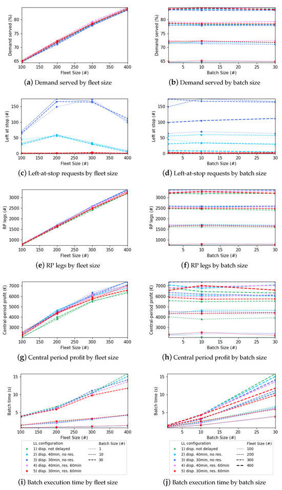
Figure 14.
Demand profile 2: analysis of demand served, left-at-stop requests, ride-pooling legs dispatched, central period profit and batch execution time according to fleet size and batch size. Source: created by the authors.
Furthermore, the analysis focuses on a batch size of 10 requests, as this number provides the best time performance, and excludes LLC3 due to its poor performance in left-at-stop requests. A fleet size of 400 vehicles is chosen as it produces a higher demand served, profitability and shorter travel times. However, the main focus is on the increase in passengers. Table 11 and Table 12 present the served, unserved and left-at-stop requests as well as the average passengers per request for each case, the ride-pooling legs served, and vehicle occupancy. The results obtained here are comparable to those observed for single-passenger demand. The service demand is slightly lower, but it still serves 2000 more passengers. There is a higher number of passengers with unserved and left-at-stop requests compared to served requests, indicating the challenge of finding suitable vehicles with the necessary capacity, as supported by increased vehicle occupancy.
Table 11.
Demand profile 2, 400V_10R experiments: summary of service demand.
Table 12.
Demand profile 2, 400V_10R experiments: summary of left-at-stop and unserved requests.
Table 13 presents the total travel times, distances and fares for each intermodal type and indicates a consistent pattern across all of the LL configurations. Only a slight increase in fares occurs, which can be attributed to the higher number of passengers per request. However, Table 14 reveals that the cost per passenger has actually improved for each individual passenger, even during RP trips, compared to single-passenger demand.
Table 13.
Demand profile 2, 400V_10R experiments: summary of mean travel times, distances and fares for each intermodal type.
Table 14.
Demand profile 2, 400V_10R experiments: summary of passengers per request and fare per passenger for each intermodal type.
Table 15 presents the profit analysis and highlights a significant difference between the LL configurations compared to single-passenger demand. Although minor losses are observed throughout the total period, delaying LL dispatch led to an increase of approximately 600 € in system profit compared to LLC1. This outcome was achieved with the new multi-passenger fare system, which rewards passengers for joining and distributes the cost among passengers travelling together.
Table 15.
Demand profile 2, 400V_10R experiments: profit analysis for the 6.5-h total period (from 8:30 a.m. to 3 p.m.) and 3.5-h central period (without warm-up and cool-down periods, from 9:30 a.m. to 1 p.m.)
Table 16 presents an overview of the service rates based on origin and destination points, request type and number of passengers. Booking requests consistently maintain a high service rate: exceeding 90% in most areas regardless of the number of passengers. However, for HN requests, there is a noticeable decrease in the service rate as the number of passengers increases, highlighting the challenge of accommodating such requests when an immediate departure is desired.
Table 16.
Demand profile 2, 400V_10R_LLC4 experiment: analysis of service demand by origin and destination point, request type and number of passengers.
7. Conclusions
This article explored various aspects of integrating a ride-pooling service with public transport, taking into account fleet size, batch size for grouping requests (using a batch dispatching approach) and a delayed dispatching technique using a vehicle reservation strategy to schedule requests based on time windows. Different demand profiles were investigated, ranging from single-passenger to multiple-passenger requests. The profitability analysis of the system reveals that the central period, characterised by peak request reception, proved to be particularly profitable. Delaying LL dispatch is recommended, as this leads to more profitable outcomes and higher demand served. However, although minor losses are observed in the total profits, this could potentially be remedied by implementing dynamic fleet size policies that can adapt to the system’s (currently unknown) demand profile, thereby gradually adhering to the warm-up and cool-down periods instead of deploying the entire fleet. Additionally, as pointed out in Section 1, the system is not intended to accommodate disruptions in the public transportation system (i.e., abrupt changes or service interruptions), representing a source of possible future research. This study found that vehicle capacity is not a limiting factor and that the inability to serve additional requests is primarily due to time window constraints rather than capacity limitations.
A generic methodology is proposed using two tools—a simulator and an optimisation model—and the methodology is applicable to almost any scenario. Its application was shown for the Barcelona metropolitan area, but it could have been applied to many other cities. Its application to another scenario may present some particularities of the transport system of the city/scenario in question. The methodology and adaptability of the model and its implementation, however, do not change thanks to the full parametrisation capability of the system.
Author Contributions
Conceptualization and methodology, E.L., E.C., J.B. and K.N.; writing—original draft preparation and formal analysis, E.L., E.C. and J.B.; software, data curation and visualization, E.L.; project administration, supervision and validation, E.C., J.B. and K.N. All authors have read and agreed to the published version of the manuscript.
Funding
This research was funded by an industrial PhD grant from the Generalitat de Catalunya and the company PTV-AG under grant DI-071 2019. This study was also a research project funded by the Spanish R+D Programs, MCIN/AEI/10.13039/501100011033, under project PID2020-112967GB-C31.
Institutional Review Board Statement
Not applicable.
Informed Consent Statement
Not applicable.
Data Availability Statement
Data sharing is not applicable to this article.
Acknowledgments
Many thanks to inLabFIB-UPC, a research laboratory of the Barcelona School of Informatics (FIB) at the Polytechnic University of Catalonia (UPC), for allowing us to use one of their machines for our experiments.
Conflicts of Interest
Authors Ester Lorente and Klaus Nökel were employed by the company PTV Group. The remaining authors declare that the research was conducted in the absence of any commercial or financial relationships that could be construed as a potential conflict of interest. authors declare no conflicts of interest.
Abbreviations
The following abbreviations are used in this manuscript:
| AN | Access node |
| B | Booking request (placed in advance) |
| DO | Drop-off |
| HN | Here-and-now request (placed immediately) |
| ITF | International transport forum |
| LL | Last leg request (request for a last leg of ride-pooling) |
| PT | Public transport |
| PU | Pick-up |
| RP | Ride-pooling |
| UITP | International Union of Public Transport |
References
- Zheng, Q. Would Uber Help to Reduce Traffic Congestion? Ph.D. Thesis, Skidmore College, Saratoga Springs, NY, USA, 2019. [Google Scholar]
- Erhardt, G.D.; Roy, S.; Cooper, D.; Sana, B.; Chen, M.; Castiglione, J. Do transportation network companies decrease or increase congestion? Sci. Adv. 2019, 5, eaau2670. [Google Scholar] [CrossRef] [PubMed]
- Diao, M.; Kong, H.; Zhao, J. Impacts of transportation network companies on urban mobility. Nat. Sustain. 2021, 4, 494–500. [Google Scholar] [CrossRef]
- UITP. Mobility as a Service; UITP Technical Report; International Association of Public Transport (UITP): Brussels, Belgium, 2019. [Google Scholar]
- UITP Policy Brief. Autonomous Vehicles: A Potential Game Changer for Urban Mobility; Technical Report; International Association of Public Transport (UITP): Brussels, Belgium, 2017. [Google Scholar]
- ITF. Shared Mobility Simulations for Auckland. In International Transport Forum Policy Papers; OECD Publishing: Paris, France, 2017; p. 114. [Google Scholar] [CrossRef]
- ITF. Shared Mobility Simulations for Dublin. In International Transport Forum Policy Papers; OECD Publishing: Paris, France, 2018; p. 95. [Google Scholar] [CrossRef]
- ITF. Shared Mobility Simulations for Helsinki. In International Transport Forum Policy Papers; OECD Publishing: Paris, France, 2017; p. 95. [Google Scholar] [CrossRef]
- Stone, T. MaaS Global Declares Bankruptcy; Traffic Technology International: London, UK, 2024. [Google Scholar]
- Liang, X.; de Almeida Correia, G.H.; van Arem, B. Optimizing the service area and trip selection of an electric automated taxi system used for the last mile of train trips. Transp. Res. Part Logist. Transp. Rev. 2016, 93, 115–129. [Google Scholar] [CrossRef]
- Stiglic, M.; Agatz, N.; Savelsbergh, M.; Gradisar, M. Enhancing urban mobility: Integrating ride-sharing and public transit. Comput. Oper. Res. 2018, 90, 12–21. [Google Scholar] [CrossRef]
- Pinto, H.K.; Hyland, M.F.; Mahmassani, H.S.; Ömer Verbas, I. Joint design of multimodal transit networks and shared autonomous mobility fleets. Transp. Res. Part Emerg. Technol. 2020, 113, 2–20. [Google Scholar] [CrossRef]
- Liu, Y.; Ouyang, Y. Mobility service design via joint optimization of transit networks and demand-responsive services. Transp. Res. Part Methodol. 2021, 151, 22–41. [Google Scholar] [CrossRef]
- Hickman, M.; Blume, K. Modeling Cost and Passenger Level of Service. In Computer-Aided Scheduling of Public Transport; Voß, S., Daduna, J.R., Eds.; Springer: Berlin/Heidelberg, Germany, 2001; pp. 233–251. [Google Scholar] [CrossRef]
- Huang, Y.; Kockelman, K.M.; Garikapati, V. Shared automated vehicle fleet operations for first-mile last-mile transit connections with dynamic pooling. Comput. Environ. Urban Syst. 2022, 92, 101730. [Google Scholar] [CrossRef]
- Maruyama, R.; Seo, T. Integrated Public Transportation System with Shared Autonomous Vehicles and Fixed-Route Transits: Dynamic Traffic Assignment-Based Model with Multi-Objective Optimization. Int. J. Intell. Transp. Syst. Res. 2023, 21, 99–114. [Google Scholar] [CrossRef]
- Kadem, K.; Ameli, M.; Zargayouna, M.; Oukhellou, L. An Analytical Approach for Intermodal Urban Transportation Network Equilibrium including Shared Mobility Services. arXiv 2024, arXiv:2402.00735. [Google Scholar] [CrossRef]
- Edirimanna, D.; Hu, H.; Samaranayake, S. Integrating On-demand Ride-sharing with Mass Transit at-Scale. arXiv 2024, arXiv:2404.07691. [Google Scholar] [CrossRef]
- Lorente, E.; Codina, E.; Barceló, J.; Noekel, K. An Approach Based on Simulation and Optimisation for the Intermodal Dispatching of Public Transport and Ride-Pooling Services. Appl. Sci. 2023, 13, 3803. [Google Scholar] [CrossRef]
- Frisch, R. Urbane Mobilität—Auf dem Weg zu Mobility on Demand. Int. Verkehrswesen Digit. Theor. Praxis Innov. Strateg. Mobilität Morgen 2018, 70, 53–54. [Google Scholar]
- Jamshidi, H. Dynamic Planning for Recharging Shared Electric Taxies. Ph.D. Thesis, Delft University of Technology, Delft, The Netherlands, 2019. [Google Scholar]
- Lorente, E.; Barceló, J.; Codina, E.; Noekel, K. An Agent-based Simulation Model for Intermodal Assignment of Public Transport and Ride Pooling Services. In Proceedings of the 2021 International Symposium on Transportation Data and Modelling (ISTDM 2021), Virtual, 21–24 June 2021. [Google Scholar]
- Lorente, E.; Barceló, J.; Codina, E.; Noekel, K. An Intermodal Dispatcher for the Assignment of Public Transport and Ride Pooling Services. Transp. Res. Procedia 2022, 62, 450–458. [Google Scholar] [CrossRef]
- Ma, S.; Zheng, Y.; Wolfson, O. T-share: A large-scale dynamic taxi ridesharing service. In Proceedings of the International Conference on Data Engineering, Brisbane, QLD, Australia, 8–12 April 2013; pp. 410–421. [Google Scholar]
- Asghari, M.; Deng, D.; Shahabi, C.; Demiryurek, U.; Li, Y. Price-Aware Real-Time Ride-Sharing at Scale: An Auction-Based Approach. In Proceedings of the SIGSPACIAL’16: 24th ACM SIGSPATIAL International Conference on Advances in Geographic Information Systems, New York, NY, USA, 31 October–3 November 2016. [Google Scholar] [CrossRef]
- Alonso-Mora, J.; Samaranayake, S.; Wallar, A.; Frazzoli, E.; Rus, D. On-demand high-capacity ride-sharing via dynamic trip-vehicle assignment. Proc. Natl. Acad. Sci. USA 2017, 114, 462–467. [Google Scholar] [CrossRef]
- Wallar, A.; Van Der Zee, M.; Alonso-Mora, J.; Rus, D. Vehicle Rebalancing for Mobility-on-Demand Systems with Ride-Sharing. In Proceedings of the 2018 IEEE/RSJ International Conference on Intelligent Robots and Systems (IROS), Madrid, Spain, 1–5 October 2018; IEEE Press: Piscataway, NJ, USA, 2018; pp. 4539–4546. [Google Scholar] [CrossRef]
- Schaller Consulting. The New York City Taxicab Fact Book; Technical Report; Schaller Consulting: New York, NY, USA, 2006; Available online: http://www.schallerconsult.com/taxi/taxifb.pdf (accessed on 2 April 2024).
- Barceló, J.; Montero, L.; Ros Roca, X. Virtual Mobility Lab: A Systemic Approach to Urban Mobility Challenges; Technical Report; UPC Commons: Barcelona, Spain, 2018; Available online: http://hdl.handle.net/2117/113344 (accessed on 2 April 2024).


Disclaimer/Publisher’s Note: The statements, opinions and data contained in all publications are solely those of the individual author(s) and contributor(s) and not of MDPI and/or the editor(s). MDPI and/or the editor(s) disclaim responsibility for any injury to people or property resulting from any ideas, methods, instructions or products referred to in the content. |
© 2024 by the authors. Licensee MDPI, Basel, Switzerland. This article is an open access article distributed under the terms and conditions of the Creative Commons Attribution (CC BY) license (https://creativecommons.org/licenses/by/4.0/).