Article

Estimation of Crash Modification Factors (CMFs) in Mountain Freeways: Considering Temporal Instability in Crash Data

1
School of Traffic and Transportation Engineering, Changsha University of Science and Technology, Changsha 410114, China
2
School of Civil Engineering, Hunan City College, Yiyang 413000, China
3
School of Transportation, Southeast University, Nanjing 211189, China
*
Author to whom correspondence should be addressed.
Sustainability 2024, 16(12), 5068; https://doi.org/10.3390/su16125068
Submission received: 22 April 2024 / Revised: 7 June 2024 / Accepted: 7 June 2024 / Published: 14 June 2024

Abstract

:
The combined contributions to mountain freeway safety of pavement performance, weather conditions, and traffic condition indicators have not been thoroughly investigated due to the complexity of their interactions and temporal instability. A cross-sectional analysis using a Generalized Linear Model (GLM) approach with negative binomial distribution considering time-correlation effects (TC-NB) was adopted to estimate the Crash Modification Factors (CMFs) of these indicators for different segment types, alignment types, and cross-sectional forms based on eight quarters of data from mountain freeways in China. According to the results, improving the pavement performance indexes positively impacts the safety of different freeway segments, especially for the curved segments. Quarterly Average Daily Traffic (QADT) has significantly negative safety effects on two-lane segments with relatively narrow spaces, while the proportion of large vehicles plays a decisive role in the safety impacts of tunnel segments. Small/moderate rain days in a quarter (SMR) were significantly positively correlated with crash frequency, while the percentage of torrential rain days in a quarter (TR) showed an opposite trend. The results of this study contribute to the effective coordination of traffic monitoring systems, pavement management systems, and traffic safety management systems to develop targeted improvement countermeasures for different freeway section types.

1. Introduction

The Crash Modification Factors (CMFs), which quantify the changes in road safety outcomes, specifically crash risk, resulting from implementing single or combined treatments, serve as one of the most critical reference indicators for traffic management authorities worldwide when preparing road safety improvement programs [1,2]. A CMF value of 1.0, for example, represents zero effect on safety in the evaluation process, whereas a CMF value greater than 1.0 indicates that the treatment results in a higher crash risk, while a CMF value less than 1.0 indicates a lower crash risk. Since the 1980s, a large number of studies have used different methods to confirm CMFs for both single and multiple safety management strategies on roads, and CMFs are gradually being recognized as good predictors of expected improvement outcomes. [3]. Observational before – after (BA) studies and the cross-sectional method are regarded as the two state-of-the-art methods for developing CMFs by the Highway Safety Manual (HSM) Volume 3, Part D (AASHTO, 2010) [4] and other studies [5,6,7,8]. Because of the following reasons, before–after study is not always practical. First, there could be insufficient before and after crash data. Second, the date of implementation of the treatment is unknown or it is difficult to distinguish the effect of the countermeasure from confounding factors [9]. The cross-Sectional approach is extremely competitive due to its data accessibility and ease of processing [10]. Establishing superior Safety Performance Functions (SPFs), which typically include counting models for crash frequency, is a prerequisite for reliable estimation of the CMFs.
Interactions of pavement performance, weather conditions, and traffic conditions combine to affect traffic safety. Over the past three decades, most studies have primarily evaluated CMFs for road design characteristics (e.g., geometric and cross-section characteristics) [1,7,11] and traffic characteristics (e.g., traffic volume, traffic composition) [10,12,13], with few CMFs considering pavement performance and weather conditions, which introduces bias for traffic management authorities when analyzing the economic benefits of road management. The introductions of efficient pavement performance and weather testing equipment have provided the opportunity to quickly obtain pavement performance indicators such as Pavement Surface Condition Index (PCI), Riding Quality Index (RQI), Skidding Resistance Index (SRI), and weather condition indicators such as the Percentage of small/moderate rainfall (SML) and the percentage of heavy/stormy rainfall (TR) [1].
It is worth noting that pavement performance, traffic characteristics, and weather conditions have significant temporal characteristics, i.e., their performance changes regularly over time (years, quarters, and months). Such changes lead to correlations of traffic crashes occurring in adjacent time units, which is known as temporal correlation [14]. Traditional SPFs (Poisson, Negative binomial, and their improved models) implicitly assume that the effects of statistically determined factors are constant (temporally stable) over time. Specifically, because crashes are relatively rare events, analysts typically aggregate crash data over time (months, quarters, or years) to provide a sufficient number of observations for statistical analysis. Thus, the time interval between two crash observations implies an assumption of temporal stability, which has far-reaching implications for the construction of SPFs and the analysis of CMFs [15].
The purpose of this study is to develop CMFs to quantify the combined effects of pavement performance, weather conditions, and traffic conditions on traffic safety on mountain freeways in China by developing innovative SPFs that consider temporal correlations in crash data.

2. Literature Review

In this section, we investigate the effects of indicators related to pavement performance, traffic conditions, and weather conditions on traffic safety and explain the sources of temporal correlations and their modeling approaches. Finally, studies that summarize the vacancies in the literature.

2.1. Impacts of Risk Factors on Traffic Safety

The main pavement performance indicators involving traffic safety include pavement skid resistance, pavement deterioration, pavement smoothness, etc. Several studies [16,17,18,19] have demonstrated that increasing the friction coefficient of pavements leads to significant positive safety effects, especially in wet pavements, intersections, and steeply sloped segments. For pavement deterioration indicators, the CMFs of Pavement Distress Ratio (DR) and Pavement Condition Index (PCI) verified that uneven pavements are prone to decreases in vehicle control, which increases the crash risks [20]. These effects are particularly pronounced on roadways with a high number of heavy vehicles [1]. Tang et al. [2] have shown that more than 60% of crashes on Chinese mountain freeways can be avoided or reduced by improving the current state of pavement deterioration. For pavement smoothness, uneven pavements increase the risk of vehicle skidding and rollover on the one hand [21], and on the other hand, they may paralyze the drainage system, resulting in excessive water on the road and increasing crash risks [22].
Traffic condition indicators affecting traffic safety mainly include traffic volume and traffic compositions. The Highway Safety Manual (HSM) [4] incorporates several Crash Modification Factors (CMFs) to quantify the change in crash frequency as a result of traffic conditions different from base conditions, primarily Annual Average Daily Traffic (AADT) and Lane Density (LD). It was found that both AADT and LD were positively correlated with crash frequency. In terms of traffic composition, most studies [23,24,25] specifically explored CMFs for heavy truck traffic, showing that heavy trucks significantly increase crash frequency due to line-of-sight obstruction. Vehicle speed is also an important factor influencing crashes. Yu et al. (2013) [26] developed CMFs for average vehicle speed on mountain freeways and found that average speed was negatively correlated with crash frequency, and this safety effect was particularly pronounced under dry seasons.
Research on the safety effects of weather conditions has been increasing in recent years. Collected meteorological data, such as annual/monthly rainfall, average/maximum/minimum temperatures, and other easily obtainable weather conditions data are widely used in road traffic safety studies [2,27,28,29,30]. For example, the results of Wen et al. (2019) [28] showed that an increase in monthly average wind speed, monthly average daily precipitation, and monthly average visibility were detrimental to freeway traffic safety. Tang et al. (2021) [2] showed that the higher the ratio of light/moderate and heavy/stormy rainfall, the higher the crash frequency in freeway tunnels, with the most pronounced effect observed for heavy/stormy rainfall. The impacts of rain on freeway safety are primarily reflected in (1) reduced visibility distance for drivers, thereby compressing the space for safe operations, and (2) reduced adhesion between the road and tires, especially on roads with heavy vehicle traffic, increasing the likelihood of heavy vehicles losing control.

2.2. Temporal Correlations in Crash Data

There is a perception in freeway safety analysis based on crash data that the influence of factors affecting crash frequency may not stabilize over time [31]. A growing number of studies have reached similar conclusions: there is at least some temporal instability in collecting a sufficient number of incident observations for statistical analysis over a given time period (annual, quarterly, or monthly), especially for risk factors with significant time series effects considered in the construction of Safety Performance Functions (SPFs), such as traffic conditions and weather conditions. For example, Malyshkina and Mannering (2010) [32] estimated Markov switching models, in which crash models alternate between two states over time. This provides statistical support for temporal instability, even over the short time periods they considered. Ignoring the transitions between states over time can lead to biased parameter estimates. Xu et al. (2014) [33] similarly found statistical support for Markov transformations in injury severity models using detailed data conditioned on crash occurrence. In addition, with the advancement of modeling methods, more methods for portraying temporal heterogeneity have emerged, including Generalized Estimating Equations (GEE) [14,15], Autoregressive Models (AM) [34], Autoregressive Moving Average Models (AMAM) [35], and Integer-valued Autoregressive Poisson models (IVAP) [36]. The common feature of these methods is to characterize the instability of risk effects by embedding correlation functions with lagged effects to portray the relationship between sample data at different time periods. It is worth noting that the AM model is simple in structure and has less impact on the original model, and thus can stand out from the many time-correlated models.

2.3. Gaps in the Literature

There are two shortcomings in the current research results. One is that the combined safety effects of pavement performance, traffic conditions, and weather conditions have not yet been reported as CMFs. As studies at this stage explore CMFs for only one or two of these risk factors, this limits the development of reliable safety improvement plans for managers. Second, considering the time-varying characteristics of the aforementioned risk factors, the SPFs in the cross-section-based estimation method of CMFs fail to provide a superior way of portraying them, resulting in significant deviations in CMF estimates from actual conditions. In response to these research gaps, this paper makes two main contributions:
(1)
The pavement performance and meteorological condition indicators of five mountainous freeways in China were investigated using multifunctional inspection vehicles and meteorological observation equipment, and combined with traffic conditions and crash data from different environments to establish a standard crash dataset representative of Chinese freeway conditions;
(2)
Autocorrelation priors were embedded into the traditional SPF structure to characterize temporal instability in the modeled data and CMFs were estimated for pavement performance, traffic conditions, and weather conditions to quantify the safety effects of each significant risk factor.

3. Data Collection and Description

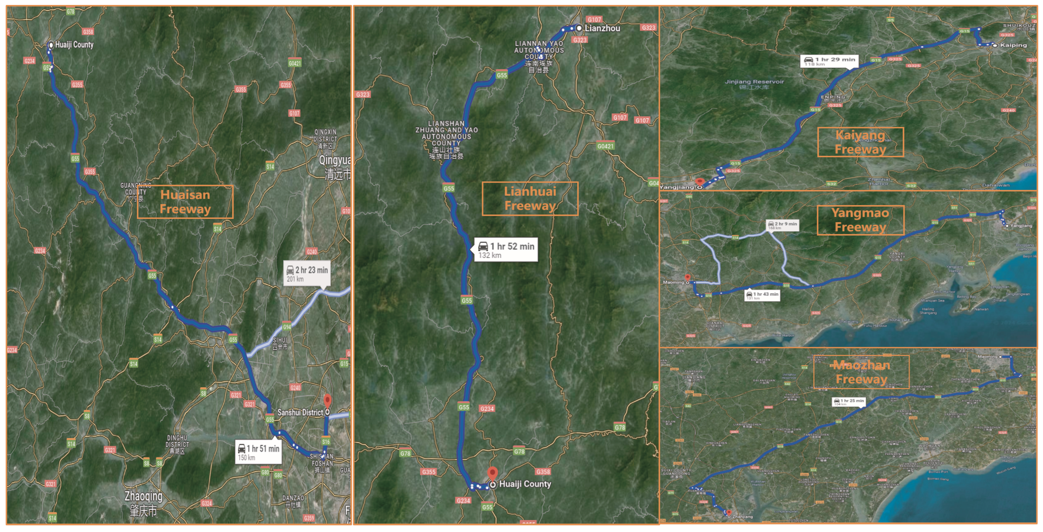
3.1. Research Objects

The database used in this paper covers five typical mountain freeways in Guangdong Province, China, including Kaiping to Yangjiang segments of the G15 Freeway (referred to as Kaiyang Freeway), Yangjiang to Maoming segments of the G15 Freeway (referred to as Yangmao Freeway), Maoming to Zhanjiang segments of the G15 Freeway (referred to as Maozhan Freeway), Lianzhou to Huaiji segments of the G55 Freeway (referred to as Lianhuai Freeway), and Huaiji to Sanshui segments of the G55 Freeway (referred to as Huaisan Freeway). The dataset was collected in the direction of Kaiping to Zhanjiang and Lianzhou to Sanshui. The route diagram and basic overview of each freeway are presented in Figure 1 and Table 1.

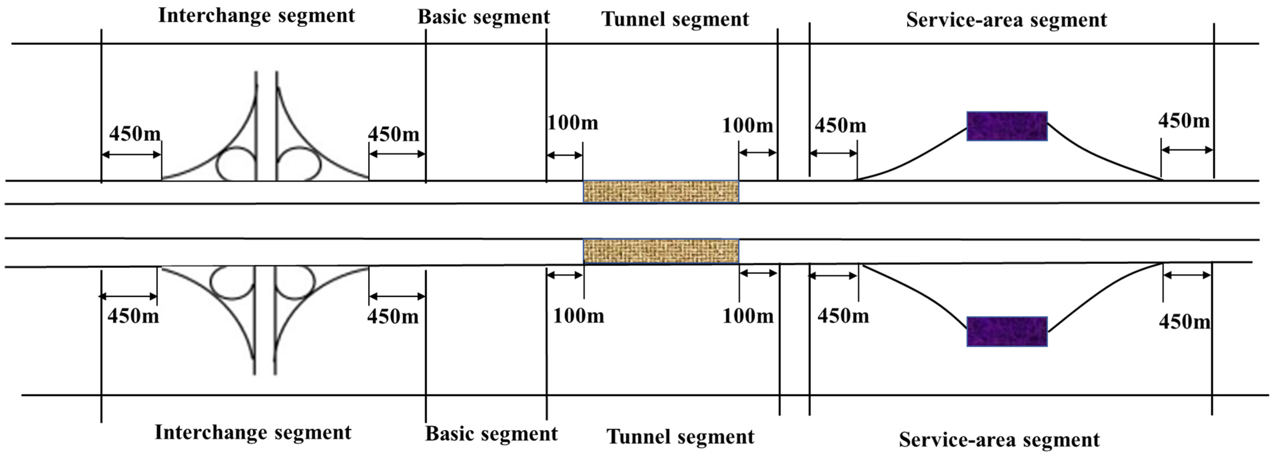
3.2. Sample Division Methods

The time scale of freeway safety analysis is mainly annual, quarterly, and monthly, while the time division unit in this paper is finally determined as quarterly for the following reasons (according to the seasonal division in southern China, February–April, May–July, August–October, and January–November in a year are defined as quarters 1–4, respectively) [2]: (1) The quarterly segmentation criterion can reduce the random interference of crashes compared to the micro-segmentation criterion represented by months. (2) The micro-segmentation criterion generates more zero-valued samples, which imposes more stringent requirements on the performance of SPFs. (3) Quarterly segmentation criteria can capture time-series type of risk factors such as pavement performance and weather conditions. Crashes and potential influencing factors for a total of eight quarters in 2015 and 2016 were used in this paper.
The spatial partitioning methods for the calibration samples of SPFs mainly include the fixed-length method and the uncertain-length method [37]. The fixed-length method divides freeways into a series of segments of the same length, usually 500 m, 1 km, or 1.5 km, by the non-overlapping equipartition method or the sliding equipartition method. Although this method is simple and efficient to operate, the values obtained after averaging indicators do not reflect the real impacts of risk factors on crashes, especially for mountainous freeways with complex conditions. The uncertain-length method cleverly circumvents this defect, which divides the freeway into segments with the same characteristic indicators but different lengths according to the principle of homogeneity. This approach does not require secondary processing of risk factor indicators for each segment, which can truly reflect the risk characteristics. Hou et al. (2018) [30] also verified that using the uncertain-length method to calibrate SPFs is more effective than that of fixed-length methods, providing a reliable basis for using the uncertain-length method in this paper.
The criteria for segmentation in this paper are truncated where the type of segment, plan geometric design, slope, and number of lane changes, and the following principles are developed. (1) The elements of smooth curves and circular curves in planar geometric design are collectively referred to as curve segments, and thus only straight segments and curve segments exist in planar geometric design. (2) The location where the slope change is greater than 1% is uniformly set as the longitudinal slope index change point, while the average slope value is used as the alternative value in the composite section where the slope change is less than 1%. (3) Segment types include basic segments, interchanges, service areas, and tunnels (as shown in Figure 2). The interchanges are defined as the area 450 m before the ramp entrance to 450 m after the ramp exit. The service area is defined as the area 450 m before the entrance to 450 m after the exit. Tunnels are defined as an area 100 m in front of the entrance to 100 m behind the exit. A total of 5568 samples (i.e., 696 × 8) were obtained by combining the initial 696 homogeneous segments with eight quarters.
Once all samples were obtained, an important task was to classify them based on the road facility environment. The purpose of this classification is to explore the variability of the safety effects of pavement performance, traffic conditions, and weather conditions across different road facility environments. Based on the clues provided by Hou et al. (2020) [37] and Cai et al. (2020) [27] special road facility segments, alignment geometry, and cross-sectional design all impact the CMFs for the risk factors discussed in this paper. For example, there is a large variability in the improvement of traffic safety for the same measures implemented on conventional freeway segments and interchanges, validating the importance of sample categorization. The selection criteria for the road facility environments in this paper include different road types (conventional segments (CS), tunnel segments (TS), interchange segments (IS), and service area segments (SAS)), straight segments (SS) and curved segments (CUS), and two-lane segments (TWS) and three-lane segments (THS). The final number of homogeneous samples obtained under each road facility environment is shown in Figure 3.
The sample sizes are strongly correlated with the standard deviation of the estimated parameters of the SPFs. In general, the larger the sample size, the smaller the standard deviation of the coefficients of each risk factor, and the more stable the variation of its CMFs across segments. As seen in Figure 3, the sample size of conventional segments dominates among all segment types, while the sample sizes of straight and curved segments, one-way two-lane segments, and one-way three-lane segments are close to each other, with slightly higher sample sizes for curved segments and three-lane segments. Based on the clues provided by the study [28], the sample sizes of all types in this paper exceed the minimum sample sizes required for crash modeling, meeting the basic requirements for CMF estimation.

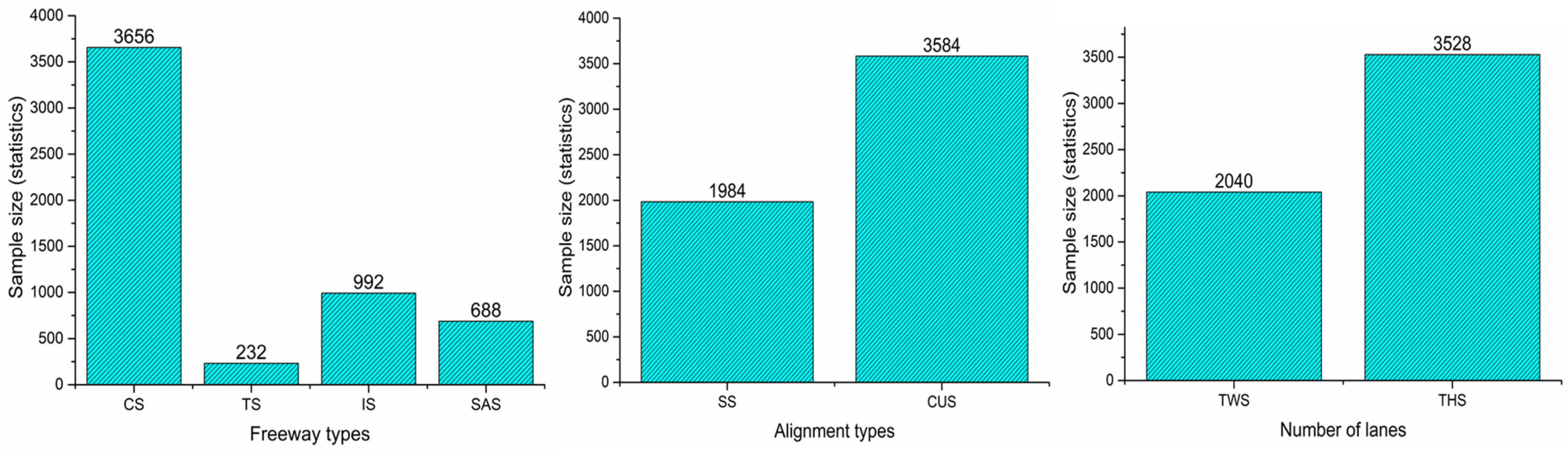
3.3. Statistical Description of Accident Modeling Data Sets

The number of crashes and risk factors were collected according to the divided segments and quarters, and a complete crash dataset was created, with statistical descriptions of each variable shown in Table 2. The following details are intended to clarify the analysis:
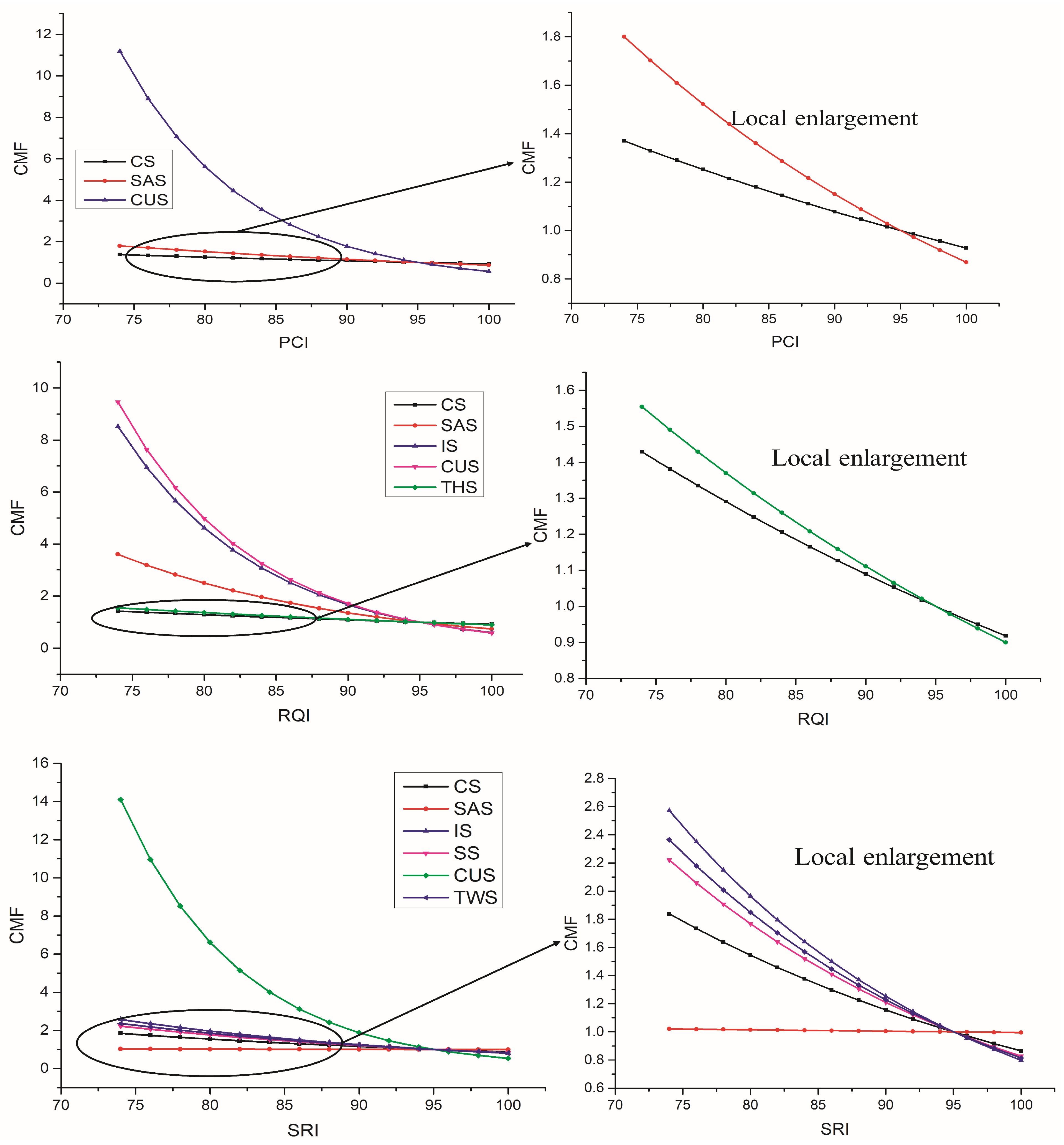
The acquisition of pavement performance indexes in Table 2 involves two steps: (1) the Pavement Distress Ratio (DR), International Roughness Index (IRI), and Sideway Force Coefficient (SFC) were obtained using a Multifunctional Road Condition Rapid Test Vehicle (SCANNER CiCS II). (2) According to the pavement performance evaluation indexes and calculation methods stipulated in the Highway Technical Condition Evaluation Standard (JTG 5210-2018) [38], the Pavement Condition Index (PCI), Riding Quality Index (RQI), Rutting Depth Index (RDI), and Skidding Resistance Index (SRI) were subsequently obtained (as shown in Table 3). The PCI represents the degree of surface damage, such as pavement cracking, potholes, and collapse, with higher PCI values indicating less surface damage. The RQI evaluates the driving quality of pavements by considering the impact of road surface roughness on driving comfort, with higher RQI values signifying better pavement leveling and driving comfort. The SRI represents the skid resistance of the pavement, derived by converting the lateral force coefficient of the pavement, where higher SRI values indicate better skid resistance;
The Guangdong Freeway Network Toll System (GFNTS) classifies vehicles into five types according to vehicle height, number of axles, number of wheels, and wheelbase (as shown in Table 4). Based on the clues provided by Wen et al. [28], the calculation of the Quarterly Average Daily Traffic Volume (QADT) and traffic compositions, whose formulas are shown in Equations (1)–(5), requires the conversion of Class 1 to Class 5 vehicles into standard traffic volumes by a coefficient of 1:1.5:2:3:3.5, respectively. According to the clues provided by Tang et al. [2], the proportion of Class 1–5 vehicles in a quarter (denoted by the symbols IVE, IIVE, IIIVE, IVVE, and VVE) is strongly associated with crash risks, forming the basis for its inclusion in the risk factors of this study. It should be noted that the proportion of Class 3 vehicles is collinear with other variables, so this variable is excluded;
The weather data, recorded on a county (district) basis, come from the Guangdong Meteorological Data Center. The freeways studied in this paper cover 41 meteorological stations, with an average distance of 36 km between them. The shortest and longest distances between meteorological stations and freeways are 18 km and 34 km, respectively. For counties (districts) containing multiple meteorological observation stations, data were averaged. The weather condition variables selected in this paper include the percentage of small/moderate rain days in a quarter (SMR), the percentage of torrential rain days in a quarter (TR), the percentage of days with no sustained wind in a quarter (WD), and the percentage of days with wind power ≥ 4 in a quarter (WP);
The crash data come from the record ledger of each freeway management center, which documents the geographical location of crashes, the cause of crashes, the related vehicle information, the severity, and the casualty situation. In the initial screening of crash data, we removed crashes caused by parking violations, spilled vehicle contents, and crashes with missing dates or locations, resulting in 1633 crashes for this study.
Q A D T k , t = V k , 1 , t + 1.5 V k , 2 , t + 2 V k , 3 , t + 3 V k , 4 , t + 3.5 V k , 5 , t Q t
V P k , 1 , t = V k , 1 , t V k , 1 , t + 1.5 V k , 2 , t + 2 V k , 3 , t + 3 V k , 4 , t + 3.5 V k , 5 , t
V P k , 2 , t = V k , 2 , t V k , 1 , t + 1.5 V k , 2 , t + 2 V k , 3 , t + 3 V k , 4 , t + 3.5 V k , 5 , t
V P k , 4 , t = V k , 4 , t V k , 1 , t + 1.5 V k , 2 , t + 2 V k , 3 , t + 3 V k , 4 , t + 3.5 V k , 5 , t
V P k , 5 , t = V k , 5 , t V k , 1 , t + 1.5 V k , 2 , t + 2 V k , 3 , t + 3 V k , 4 , t + 3.5 V k , 5 , t
where V k , 1 , t V k , 5 , t represent the number of vehicles of category 1 to 5 passing through the toll section in quarter t ( t = 1 ,   2 , ,   8 ). Q t represents the number of days in the quarter t . Q A D T k , t represents the average daily standard traffic flow of segment k in quarter t . V P k , 1 , t , V P k , 2 , t , V P k , 4 , t and V P k , 5 , t represent the proportions of class 1, 2, 4, and 5 vehicles in segment k and quarter t, respectively.

4. Methodology

4.1. Model Description

This study used SPFs that consider temporal correlations to develop CMFs for different segment types (conventional segments, interchange segments, tunnel segments, service area segments), geometric design conditions (straight and curved segments), and the number of lanes (two-lane segments and three-lane segments). SPFs were employed to quantify the effects of specific variables on the occurrence of crashes, and then CMFs were derived from the model coefficients. A recent study showed that cross-sectional studies based on regression models can provide reliable estimates of CMFs, offering valuable insights for the selection of SPFs in this paper [8].
SPFs are developed based on the premise that set count values for a specific time interval (annual, quarterly, monthly, etc.), such data decomposition generates temporal correlation and observations may be interdependent [39]. Traditional regression models implicitly assume that the effects of statistically identified determinants are constant (temporally stable) over time, introducing some bias in the results inferred for CMFs [31]. To eliminate the effects of this time stability assumption, this study embedded time correlation effects into the traditional negative binomial (NB) model to form a first-order autoregressive model.
Assuming that the crash frequency of segment i in time t follows the NB distribution, the probability distribution of Y i , t = y i , t is:
p Y i , t = y i , t = ( 1 / α 1 / α + η i , t ) 1 / α Γ ( 1 / α + y i , t ) Γ ( 1 / α ) y i , t ! ( λ i , t 1 / α + λ i , t ) y i , t
where α is the overdiscretized parameter of NB distribution; λ i , t is the expected crash frequency, which represents the product of crash chance e i , t and crash risk u i , t (as shown in Equation (7)). e i , t   is defined as the product of powers of segment lengths L i and Q A D T i (as shown in Equation (8)), and u i , t is assumed to have a generalized linear association with potential crash risk factors (as shown in Equation (9)).
λ i , t = e i , t u i , t
e i , t = ( L i ) α 1 ( Q A D T i ) α 2
I n   u i , t = β 0 + m = 1 M β m x m , i , t
where α 1 and α 2 are the coefficients to be estimated, x m , i , t is the observed value of the m t h risk factor in segment i and in quarter t , β m is its corresponding regression coefficient, M   is the total number of risk factors; and β 0 is a constant term.
The above-shown equations can be combined to obtain
I n   λ i , t = α 1 I n   L i + α 2 I n   Q A D T i , t + β 0 + m = 1 M β m x m , i , t
Equations (6)–(10) represent the complete structure of the NB model, which is also the basic model in the field of crash frequency modeling. Several studies have illustrated the increasing inappropriateness of NB models for analyzing CMFs of risk factors in complex environments. The main reason is that the fixed time effects assumption contradicts the temporal instability present in the data structure, affecting the reliability of risk factor inferences [40]. Specifically, Equation (10) assumes that the parameters β m are independent of each other, which is seriously contrary to the actual situation. A practical example fully validates this conclusion: pavement performance (PCI, RQI, SRI) decreases regularly over time, indicating a correlation between pavement performance indicators in neighboring quarters, which in turn leads to a strong correlation between crash frequencies in different quarters. Therefore, to obtain reliable CMFs, the temporal correlation of crash data must be taken into account by SPFs.
To explain this temporal correlation, this study adds the residual term ɸ i , t   with a first-order hysteresis effect to Equation (10), and the crash frequency still obeys an NB distribution with mean λ i , t :
I n   λ i , t = α 1 I n   L i + α 2 I n   Q A D T i , t + β 0 m = 1 M β m x m , i , t + ɸ i , t
Under the assumption of temporal correlations, the structured time effects ɸ i , t   obeys a normal distribution:
ɸ i , 1 ~ N ( 0 ,   2 1 γ 2 )
ɸ i , t ~ N ( γ ɸ i , t 1 ,   2 ) ,   t > 1
where γ is the autocorrelation coefficient and is the standard deviation of the time term. Equations (6)–(9) combined with Equations (11)–(13) are the complete structure of the time-correlated NB (TC-NB) model.
The most important feature of TC-NB is the embedding of random parameters with time-series effects ɸ i , t in the model structure, which to some extent captures the changing patterns of pavement performance, weather conditions, and traffic conditions with the seasons.
The CMFs were inferred from the estimated model parameters of the count model, i.e., coefficients; as the model form is log-linear, the CMFs were calculated as the exponent of the associated coefficient of the countermeasure variable as presented in Equation (14) [1,41]:
C M F K = e x p ( β k X k r X k b )
where X k r is the range of values for roadway characteristic k , and X k b is the baseline condition for roadway characteristic k (when needed or available).

4.2. Parameter Estimation Method and Goodness-of-Fit Measures

The parameter estimation method of the candidate models is full Bayesian estimation, which is implemented in the WinBUGS 1.4.3 platform based on the R language. WinBUGS is one of the most reliable tools for implementing Bayesian estimation methods, which infer the posterior mean of the parameters by virtue of Markov chain Monte Carlo (MCMC) simulation and the Metropolis–Hastings algorithm [28]. Since there is no reliable prior information, all regression coefficients α 1 , α 2 , β 1 and autocorrelation coefficients γ in the candidate models are assigned uninformative prior distributions N ( 0 , 10,000 ) , the parameter 1 / 2 is given as a priori Gamma distribution G ( 0.001 , 0.001 ) . Set 1 chain for 180,000 Markov chain Monte Carlo simulation iterations and discard the first 15,000 simulation iterations. The convergence of MCMC simulation is judged by the Gelman–Rubin statistics in WinBUGS.
The three most classical test indicators of the crash model’s goodness of fit are the Deviation Information Criterion (DIC), Mean Absolute Deviation (MAD), and Root Mean Square Error (RMSE). DIC is one of the comprehensive quantitative indicators of the goodness of fit and complexity of the models [2]. MAD denotes the mean of the absolute value of the difference between the actual observed value and the posterior mean across all samples [2]. RMSE represents the mean of the square root of the difference between the actual observed value and the posterior mean across all samples [27]. The smaller the abovementioned test indexes are, the better the goodness of fits are. The specific calculation method of each performance test index is as follows:
D I C = D ¯ + P D
M A D = 1 I X T i = 1 I t = 1 T | y i , t ¯ y i , t |
R M S E = i = 1 I t = 1 T ( y i , t ¯ y i , t ) 2 / N
where D ¯ is the posterior average deviation used to represent the model fitting degree; P D is the number of valid parameters used to measure the complexity of the models; N is the number of samples; I is the total number of segments, T is the total number of quarters; y i , t ¯ represent the predicted value of crash frequency of the segment i in the time period t ; and y i , t represent the actual value of crash frequency of the segment i in the time period t .

5. Results and Analysis

5.1. Explanatory of Temporal Instability

To verify the superiority of the temporal correlation method proposed in this paper, the NB model and TC-NB model were used to calibrate all the data sets established in this paper. The applicability of the TC-NB model was verified with DIC, MAD, and RMSE and time-correlated parameters γ and ∧, and the results are shown in Table 5.
Two conclusions can be summarized from Table 5. (1) The TC-NB model has smaller DIC, MAD, and RMSE values than the corresponding NB model for all freeway environments, indicating that the TC-NB model has a better goodness-of-fit for the same dataset. This finding is within expectation and consistent with the results of research [14,39,42], suggesting that the temporal term in the lag-1 structure can consistently characterize the temporal correlations present in the data structure, especially for variables with significant time-series characteristics such as traffic conditions, pavement performance, and weather conditions. (2) Both γ and   are significant at the 90% or 95% Bayesian intervals, verifying that temporal correlations in the data structure can be explained by the lag-1 structure proposed in this paper. This indicates that the effects of traffic conditions, pavement performance, and weather conditions on traffic safety change with the seasons.

5.2. Analysis of Parameter Estimation Results for SPFs

The optimal TC-NB model was used as a benchmark to explore the parameter estimation results, as shown in Table 6. The effects of pavement performance on safety vary significantly across freeway environments: (1) All pavement performance indicators have significant negative safety effects in the CS, SAS, and CUS. (2) RQI and SRI have significant safety effects in the IS. (3) Only one of the pavement performance indicators is significantly negatively associated with traffic safety in the SS, TWS, and THS. (4) It is worth noting that pavement performance in the TS has no effects on traffic safety, which is consistent with the results of Hou et al. (2020) [30], suggesting that the lower speed of vehicles traveling in the tunnel segments eliminates some of the significant safety effects of pavement performance. In addition, the closed environment allows the tunnel pavement to avoid the erosive effects of sunlight and precipitation, which to some extent helps protect the pavement.
In terms of traffic conditions, all variables were significantly correlated with crash frequency in all segment types, except for IIVE, which had no significant safety effect under TS, i.e., QADT, IVE, and VVE are significantly positively correlated with crash frequency, while IIVE and IVVE have opposite safety effects. This finding is consistent with the results of Wen et al. (2019) [28], where the structural composition of the traffic system directly impacts its stable operation, which in turn can affect traffic safety.
In terms of weather conditions, SMR was positively associated with crash frequency in the segment types of CS, SAS, SS, CUS, and THS, while TR was negatively associated with crash frequency in the segment types of CAS, TS, CUS, TWS, and THS. This finding is consistent with Tang et al. (2021) [2], which stated that small/moderate rain elevates crash risk by reducing driving visibility and damaging road conditions, while heavy rainstorms reduce crash risk by affecting travel patterns.

5.3. Analysis of CMFs

In order to understand the CMFs of various indicators, we calculated the minimum and maximum CMFs under different base values.

5.3.1. Pavement Performance

As shown in Table 7 and Figure 4, when the PCI value decreases from 91 to 82, the average crash rates in the CS, SAS, and CUS increased by 14.45%, 28.66%, and 181.51%, respectively. This conclusion is consistent with Tang et al. (2021) [2], indicating that pavement deterioration directly affects driver stability and vehicle driving conditions. Particularly when a sharp turn is required, poor pavement conditions significantly increase the likelihood of vehicle overturning. From the CMFs of the RQI index, it is clear that driving comfort has significant safety effects in multiple environments (CS, SAS, SS, TWS, CUS), and such safety effects are significantly higher in interchange and curve segments than in conventional and service area segments. Specifically, when the RQI decreased from 91 to 82, the average crash rates of CS, SAS, SS, TWS, and CUS increased by 16.53%, 73.15%, 150.43%, 161.95%, and 20.80%, respectively. These results are consistent with the findings of Wang et al. (2020) [36], which indicate that frequent lane changes and speed shifts in interchanges, steering behavior in curved segments, and narrow maneuvering space in two-lane segments demand high roadway smoothness. A slight dip in smoothness in these segments leads to a sharp increase in crash frequency. As shown by the CMFs of the SRI index, the skid resistance of pavement significantly affects traffic safety in six traffic environments (CS, SAS, IS, SS, CUS, and TWS), with curved segments exhibiting the most pronounced safety effects: when the SRI value of pavement decreased from 91 to 82, the average crash rates of CS, SAS, IS, SS, CUS, and TWS increased by 29.8%, 2.74%, 49.93%, 40.78%, 210.81%, and 44.63%, respectively. According to Roy et al. (2023) [17] and Hussein et al. (2021) [43], who conducted an EB before–after study, deceleration and lane change behaviors on interchange segments are highly susceptible to driving instability on sections with poor skid resistance, thus increasing the likelihood of crashes. The least sensitive safety effects of SRI indicators on service area segments may result from heterogeneity and data endogeneity [30].

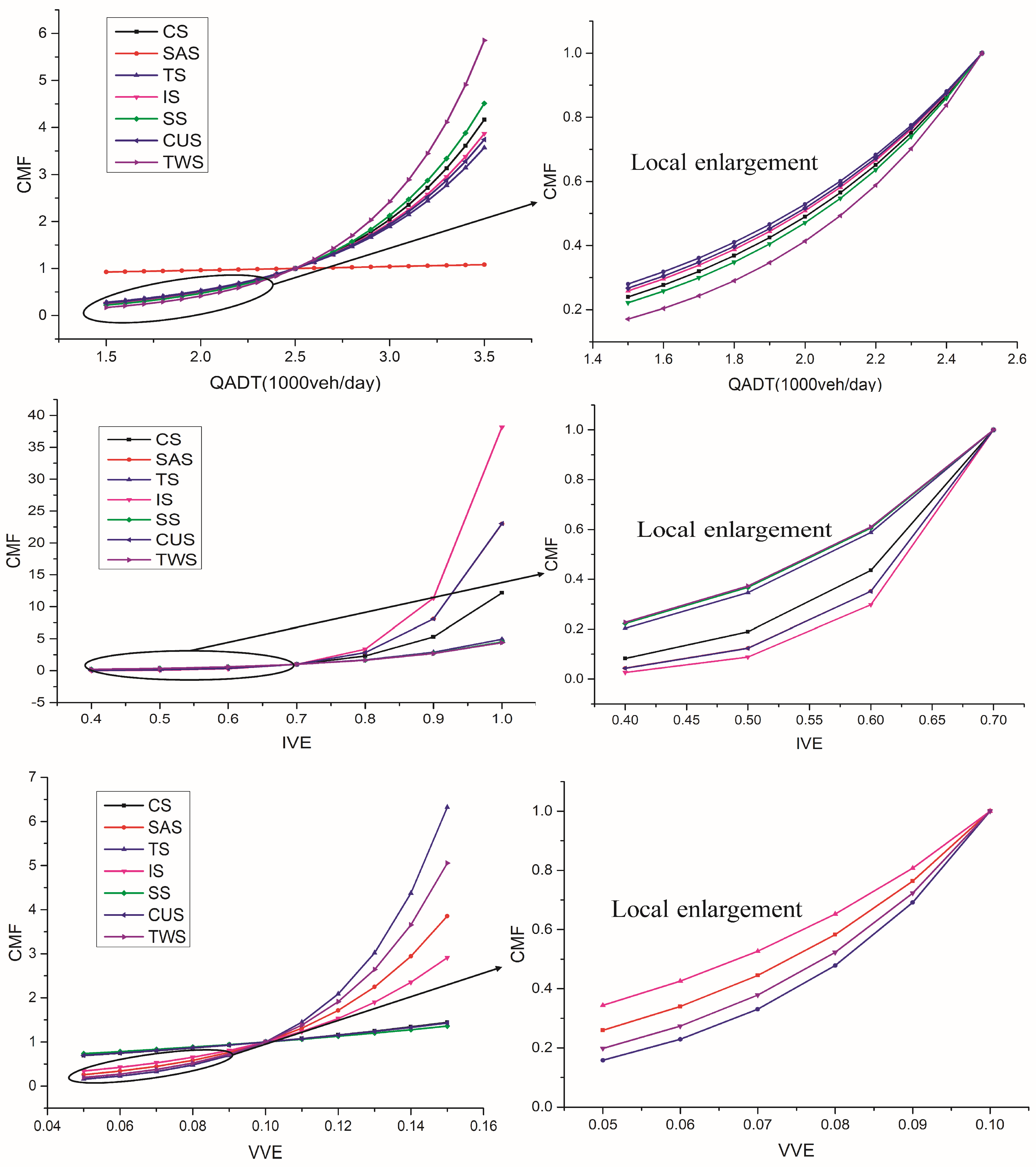
5.3.2. Traffic Conditions

As shown in Table 8 and Figure 5, the CMFs for the QADT indicate that traffic volume significantly affects safety in all road environments, particularly in two-lane segments: when QADT decreased from 3 (1000 vehicles/day) to 0.24 (1000 vehicles/day), the average crash rates reduced by 57.25%, 4.57%, 53.41%, 55.59%, 59.51%, 54.71%, 65.36%, and 44.32% for CS, SAS, TS, IS, SS, CUS, TWS, and THS, respectively. This conclusion is similar to those of several studies [18,25,30] and aligns with real-world observations: higher traffic volume constricts the operating space of vehicles and reduces the stability of the traffic system, thereby increasing the likelihood of accidents. Particularly for two-lane segments, where the driving space is already relatively small, the impact of traffic volume on safety is especially pronounced. It follows that regular highway level of service assessments are essential, along with discussions on whether to undertake renovation and expansion projects. When IVE decreased from 70% to 20%, the average accident rates reduced by 56.50%, 64.84%, 41.19%, 70.29%, 39.43%, 64.86%, 38.98%, and 50.04% for CS, SAS, TS, IS, SS, CUS, TWS, and THS, respectively. This finding is similar to the literature [2,28] indicating that more Class I vehicles increase the frequency of overtaking and lane changing, thereby increasing the likelihood of crashes. Additionally, more frequent lane-changing and lane-shifting behaviors in the weaving areas of interchanges exacerbate these safety effects. Similarly, the proportion of Class V vehicles showed significant positive correlations with crash frequency in all environments, with these safety effects being more pronounced in tunnel segments than in conventional, interchange, and service area segments; in one-way two-lane segments than in one-way three-lane segments; and in curved segments than in straight segments. Specifically, when VVE decreased from 10% to 8%, the average crash rates reduced by 13.64%, 41.71%, 52.17%, 34.78%, 11.58%, 13.34%, 47.70%, and 17.92% for CS, SAS, TS, IS, SS, CUS, TWS, and THS, respectively. The findings of Tang et al. (2021) [2] and Wen et al. (2019) [28] support this paper’s viewpoint that Class V vehicles, characterized by slow speed, large size, and sluggish braking effects, lead to instabilities such as large speed differences and restricted visibility within the traffic system, thereby elevating crash risk. The closed environment of tunnel segments, restricted visibility of curved segments, and limited operating space of one-way two-lane roads all exacerbate the sensitivity of such safety effects.

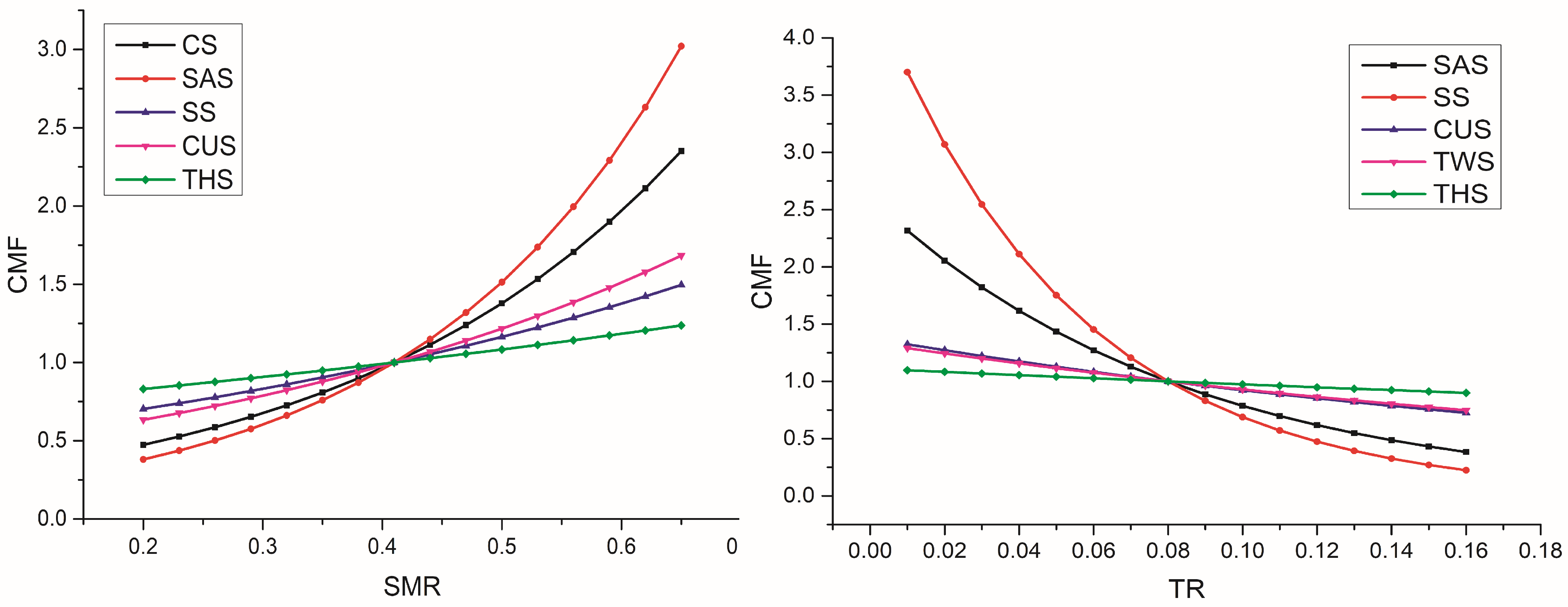
5.3.3. Weather Conditions

As shown by the CMFs of SMR, the percentage of light/medium rainfall in a season significantly impacts the safety of CS, SAS, SS, and THS (as shown in Table 9 and Figure 6), with these impacts being more pronounced for interchange segments: when the SMR is reduced from 40% to 10%, the average crash rates reduce by 65.38%, 74.89%, 39.55%, and 23.27% for CS, SAS, SS, and THS, respectively. Sawtelle et al. (2023) [44] showed that the monthly average daily precipitation on Chinese freeways is positively correlated with crash frequency, supporting this paper’s view. In fact, the impacts of rain on freeway safety are mainly reflected in (1) reduced visibility for drivers, thus compressing the space for safe operation, and (2) reduced traction between the road surface and tires, especially in segments with more heavy vehicles, which are more likely to lose control. For service area segments, frequent lane changes and speed variations exacerbate the instability of the traffic system, thus increasing the negative safety effects of rain. Cai et al. (2022) [27] proposed measures to improve road safety in rainy weather, providing a good reference for using dynamic speed-limiting strategies to mitigate unstable road–tire contact and enhance driving maneuvering space, thereby eliminating some rain-induced risky driving behaviors. Additionally, TR’s CMFs indicate that heavy rainfall actually improves freeway traffic safety: when TR increases from 7% to 12%, the average crash rates of SAS, TS, CUS, TWS, and THS reduce by 45.14%, 86.93%, 16.29%, and 6.41%, respectively. The findings of Wen et al. (2019) [28] explain these phenomena well: (1) heavy or stormy rains prevent people from planning their trips, indirectly reducing traffic volume on the highway and therefore the likelihood of accidents. (2) Heavy or stormy rains further enhance drivers’ alertness, which in turn enhances driving safety.

6. Discussing

The innovative model, which considers temporal correlation, proposed in this study provides reliable SPFs for the estimation of CMFs for risk factors with significant temporal effects. The significance of this innovative model is not limited to the analysis of CMFs on mountain freeways but also extends to various scenarios such as urban intersections and rural roads, provided there are temporal effects on the risk factors [45].
The CMFs for pavement performance indicators suggest that pavement preservation measures, whether aimed at increasing friction and smoothness or reducing pavement damage, will positively impact safety, particularly on curved segments and interchanges. This conclusion’s deeper significance lies in the ability of traffic managers to prioritize limited funds toward improving pavement performance on highway segments with sharp curves and interchanges, while selectively improving other segments based on the remaining funds [1].
A practically significant result is that large vehicles pose extreme risks at mountainous freeway entrances and exits, a factor often overlooked by most transportation agencies in their safety evaluation procedures during the design and operation phases of freeways. [46]. Although the addition of control facilities for large vehicles will increase the daily operation cost, the crash risk reduction can be estimated by the CMF of this study. It is strongly recommended that the cost–benefit ratios of corrective large-vehicle control measures be estimated for safety improvements at highway entrances and exits in mountainous areas of China. If the cost–benefit values are favorable, this intervention should be routinely implemented to significantly reduce the economic losses and negative social impacts caused by serious collisions with large vehicles and the resulting congestion.
The incorporation of refined meteorological data provides valuable foresight for safety management systems, allowing management units to dynamically adjust control measures based on the CMFs of meteorological parameters. For example, traffic control restrictions can be imposed at highway entrances and exits before the arrival of light/moderate rainfall to enhance road safety. Another interesting finding that warrants extended study by researchers is that rainstorms can instead promote traffic safety. We speculate that this is due to human factors, such as changes or interruptions in travel plans and increased driving caution. Thus, with limited funding, transportation managers can implement distinct improvement measures for light to moderate rain and heavy rain, focusing on traffic restriction measures to reduce accidents during light to moderate rain and fast rescue measures to mitigate impacts after accidents in heavy rain [27,28].
It should be noted that the reason this study is based on data from typical mountain highways in China is that the driving environment of mountainous highways is relatively complex, and the interactions between pavement performance, traffic conditions, and weather conditions are more pronounced. For other regions or types of highways (e.g., highways in flat terrain regions in northern China), the value of this study lies in providing a set of methodological templates for estimating CMFs for risk factors with time-varying patterns. When other regions or types of highways follow the data processing and CMF estimation methods provided in this paper, reliable traffic safety effects of each risk factor can also be obtained.

7. Conclusions

Using data from typical mountain expressways in China, this study employed SPFs fitted with generalized linear modeling techniques and a negative binomial distribution error structure, incorporating time-related parameters, to develop CMFs for pavement performance, traffic conditions, and weather indicators for different facility types (e.g., conventional segments, tunnel segments, interchange segments, and service area segments), alignment types (e.g., straight and curved segments), and cross-section types (e.g., one-way two lanes and one-way three lanes). CMFs for the following parameters were developed: PCI, RQI, SRI, QADT, IVE, VVE, SMR, and TR.
The main conclusions of this paper include the following. (1) The NB model with embedded auto-correlation regression function (TC-NB) has superior goodness-of-fit (DIC, MAD, RMSE) compared to the traditional NB model, demonstrating its ability to capture time-correlated features of the crash dataset, thereby providing superior safety performance functions (SPFs) for estimating CMFs. (2) In terms of CMFs for pavement performance indicators, improving the pavement condition index (PCI) has positive safety effects, with curved segments benefiting the most. Enhanced driving comfort (RQI) has significant positive safety effects, with significantly greater effects on interchanges and curved segments than on conventional segments and service areas. Improved skid resistance (SRI) is decisive for increasing the level of safety on curved segments. (3) In terms of CMFs for traffic condition indicators, controlling traffic volumes (QADT) is effective in reducing crash risks, especially on two-lane segments. Measures to control the proportion of heavy vehicles can significantly reduce the crash risks on highways, with more pronounced improvements on one-way two-lane roads, tunnel segments, and curved segments. (4) The proportion of light/moderate rainfall in a season has a significant effect on the safety of CS, SAS, SS, and THS, and these effects are more pronounced for the interchanges. Stormy weather is beneficial for improving highway traffic safety due to changes in human travel plans and increased driving alertness.
Our study results allow us to effectively integrate pavement management systems and safety management systems. The role of pavement condition in highway safety can be further emphasized based on CMFs when developing pavement management systems and maintenance programs, in addition to considering life-cycle cost analyses and pavement condition objectives. The opportunity for pavement monitoring provided by high-efficiency equipment and technological advancements makes the availability of CMFs for both pavement surface and traffic condition parameters crucial and adds significant value in maintaining pavement conditions and improving traffic characteristics considering their safety effects. In addition, the incorporation of refined meteorological data provides reliable foresight for the safety management system, and management units can dynamically adjust control measures based on the CMF of meteorological parameters.
Further research could be conducted in two ways. The first is to continue to expand the standardized crash dataset, preferably by including human risk factors (driving age, DUI or not, route familiarity, etc.) in the discussion of CMFs to form a full-factor crash data set that encompasses “human–vehicle–road–environment”. The second is to investigate the spatial heterogeneity within the modeling samples by correlating the risk factors of adjacent road segments using hierarchical modeling techniques, spatial autoregression techniques, etc. to overcome the limitation of assuming spatial independence among the samples.

Author Contributions

L.Z.: conceptualization, methodology, validation, writing—original draft, writing—review and editing, supervision, funding acquisition. Z.H.: conceptualization, methodology, validation, supervision, funding acquisition. A.K.: investigation, formal analysis, data curation, writing—original draft, writing—review and editing. J.Y.: formal analysis, data curation, writing—original draft, writing—review and editing. M.C.: formal analysis, data curation, writing—original draft, writing—review and editing. All authors have read and agreed to the published version of the manuscript.

Funding

(1) National Natural Science Foundation of China (No. 52302429, No. 52302385); (2) Scientific Research Fund of Hunan Provincial Education Department (No. 22B0325); (3) Open Fund of Engineering Research Center of Catastrophic Prophylaxis and Treatment of Road & Traffic Safety of Ministry of Education (Changsha University of Science & Technology) (No. kfj220403); (4) the Foundation of Hunan Province Educational Committee (grant No. 22C0173).

Institutional Review Board Statement

Not applicable.

Informed Consent Statement

Not applicable.

Data Availability Statement

The data presented in this study are available on request from the corresponding author.

Acknowledgments

The authors would like to acknowledge with sincere thanks the Guangdong Transportation Group for providing the raw data and their invaluable cooperation throughout the course of the project.

Conflicts of Interest

The authors declare no conflicts of interest.

References

  1. Cafiso, S.; Montella, A.; D’Agostino, C.; Mauriello, F.; Galante, F. Crash modification functions for pavement surface condition and geometric design indicators. Accid. Anal. Prev. 2021, 149, 105887. [Google Scholar] [CrossRef]
  2. Tang, F.; Fu, X.; Cai, M.; Lu, Y.; Zhong, S. Investigation of the Factors Influencing the Crash Frequency in Expressway Tunnels: Considering Excess Zero Observations and Unobserved Heterogeneity. IEEE Access 2021, 9, 2169–3536. [Google Scholar] [CrossRef]
  3. Al-Marafi, M.N.; Somasundaraswaran, K. A review of the state-of-the-art methods in estimating crash modification factor (CMF). Transp. Res. Interdiscip. Perspect. 2023, 20, 100839. [Google Scholar] [CrossRef]
  4. AASHTO. Highway Safety Manual. 2010, p. 20. Available online: https://www.highwaysafetymanual.org/Pages/support_answers.aspx (accessed on 15 January 2024).
  5. Davis, G.A. Mechanisms, mediators, and surrogate estimation of crash modification factors. Accid. Anal. Prev. 2021, 151, 105978. [Google Scholar] [CrossRef]
  6. Mbatta, G. Developing Crash Modification Factors for Urban Highway with Substandard Wide Curb Lane; Florida State University: Tallahassee, FL, USA, 2017. [Google Scholar]
  7. Vinayaraj, V.S.; Perumal, V. Developing Safety Performance Functions and Crash Modification Factors for Urban Roundabouts in Heterogeneous Non-Lane-Based Traffic Conditions. Transp. Res. Rec. 2023, 8, 644–661. [Google Scholar] [CrossRef]
  8. Gayah, V.V.; Donnell, E.T.; Zhang, P. Crash modification factors for high friction surface treatment on horizontal curves of two-lane highways: A combined propensity scores matching and empirical Bayes before-after approach. Accid. Anal. Prev. 2024, 199, 107536. [Google Scholar] [CrossRef]
  9. Park, J.; Abdel-Aty, M.; Wang, J.; Lee, C. Assessment of safety effects for widening urban roadways in developing crash modification functions using nonlinearizing link functions. Accid. Anal. Prev. 2015, 79, 80–87. [Google Scholar] [CrossRef]
  10. Galgamuwa, U.; Vahl, C.I.; Dissanayake, S. Role of driver behaviors and environmental characteristics in evaluating safety effectiveness of roadway countermeasures: A novel approach of estimating crash modification factors. J. Transp. Saf. Secur. 2020, 12, 764–781. [Google Scholar] [CrossRef]
  11. Park, J.; Abdel-Aty, M.; Lee, J. Developing crash modification functions to assess safety effects of adding bike lanes for urban arterials with different roadway and socio-economic characteristics. Accid. Anal. Prev. 2015, 74, 179–191. [Google Scholar] [CrossRef] [PubMed]
  12. Zhao, J.; Kargel, A.; McDaniel-Wilson, C.; Kolody, K.; Zhou, H. Evaluating Safety Treatments with Crash Modification Function: Case Study on Combined Safety Treatments for Rural Two-Lane Highways. J. Transp. Eng. Part A Syst. 2023, 149, 04023021. [Google Scholar] [CrossRef]
  13. Chen, Y.; Wu, L.; Huang, Z. Assessing quality of crash modification factors estimated by empirical Bayes before-after methods. J. Cent. South Univ. 2020, 27, 2259–2268. [Google Scholar] [CrossRef]
  14. Yan, X.; He, J.; Zhang, C.; Wang, C.; Ye, Y.; Qin, P. Temporal instability and age differences of determinants affecting injury severities in nighttime crashes. Anal. Methods Accid. Res. 2023, 38, 100268. [Google Scholar] [CrossRef]
  15. Alnawmasi, N.; Ali, Y.; Yasmin, S. Exploring temporal instability effects on bicyclist injury severities determinants for intersection and non-intersection-related crashes. Accid. Anal. Prev. 2024, 194, 107339. [Google Scholar] [CrossRef]
  16. Cafiso, S.; D’Agostino, C.; Delfino, E. From manual to automatic pavement distress detection and classification. In Proceedings of the 2017 5th IEEE International Conference on Models and Technologies for Intelligent Transportation Systems (MT-ITS), Naples, Italy, 26–28 June 2017; pp. 433–438. [Google Scholar]
  17. Roy, U.; Farid, A.; Ksaibati, K. Effects of Pavement Friction and Geometry on Traffic Crash Frequencies: A Case Study in Wyoming. Int. J. Pavement Res. Technol. 2023, 16, 1468–1481. [Google Scholar] [CrossRef]
  18. Montella, A.; Chiaradonna, S.; Criscuolo, G.; De Martino, S. Development and evaluation of a web-based software for crash data collection, processing and analysis. Accid. Anal. Prev. 2019, 130, 108–116. [Google Scholar] [CrossRef]
  19. Angelo, A.A.; Sasai, K.; Kaito, K. Assessing Critical Road Sections: A Decision Matrix Approach Considering Safety and Pavement Condition. Sustainability 2023, 15, 7244. [Google Scholar] [CrossRef]
  20. Chen, S.; Saeed, T.U.; Labi, S. Impact of road-surface condition on rural highway safety: A multivariate random parameters negative binomial approach. Anal. Methods Accid. Res. 2017, 16, 75–89. [Google Scholar] [CrossRef]
  21. Khayesi, M. The Handbook of Road Safety Measures. Inj. Prev. 2006, 12, 63–64. [Google Scholar]
  22. Chan, C.; Huang, B.; Yan, X.; Richards, S. Investigating effects of asphalt pavement conditions on traffic accidents in Tennessee based on the pavement management system (PMS). J. Adv. Transport. 2010, 44, 150–161. [Google Scholar] [CrossRef]
  23. Chen, S.; Chen, Y.; Xing, Y. Comparison and analysis of crash frequency and rate in cross-river tunnels using random-parameter models. J. Transp. Saf. Secur. 2022, 14, 280–304. [Google Scholar] [CrossRef]
  24. Cheng, W.; Gill, G.S.; Zhou, J.; Ensch, J.L.; Kwong, J.; Jia, X. Alternative multivariate multimodal crash frequency models. J. Transp. Saf. Secur. 2019, 12, 628–652. [Google Scholar] [CrossRef]
  25. Aguilar, C.; Russo, B.J.; Mohebbi, A.; Akbariyeh, S. Analysis of factors affecting the frequency of crashes on interstate freeways by vehicle type considering multiple weather variables. J. Transp. Saf. Secur. 2022, 14, 973–1001. [Google Scholar] [CrossRef]
  26. Yu, R.; Abdel-Aty, M. Utilizing support vector machine in real-time crash risk evaluation. Accid. Anal. Prev. 2013, 51, 252–259. [Google Scholar] [CrossRef] [PubMed]
  27. Cai, M.; Tang, F.; Fu, X. A Bayesian Bivariate Random Parameters and Spatial-Temporal Negative Binomial Lindley Model for Jointly Modeling Crash Frequency by Severity: Investigation for Chinese Freeway Tunnel Safety. IEEE Access 2022, 10, 38045–38064. [Google Scholar] [CrossRef]
  28. Wen, H.E.A.; Zhang, X.; Zeng, Q.; Sze, N.N. Bayesian spatial-temporal model for the main and interaction effects of roadway and weather characteristics on freeway crash incidence. Accid. Anal Prev. 2019, 132, 105249. [Google Scholar] [CrossRef] [PubMed]
  29. Wang, J.; He, S.; Zhai, X.; Wang, Z.; Fu, X. Estimating mountainous freeway crash rate: Application of a spatial model with three-dimensional (3D) alignment parameters. Accid. Anal. Prev. 2022, 170, 106634. [Google Scholar] [CrossRef] [PubMed]
  30. Hou, Q.; Tarko, A.; Meng, X. Investigating factors of crash frequency with random effects and random parameters models: New insights from Chinese freeway study. Accid. Anal. Prev. 2018, 120, 1–12. [Google Scholar] [CrossRef] [PubMed]
  31. Islam, M.; Alnawmasi, N.; Mannering, F. Unobserved heterogeneity and temporal instability in the analysis of work-zone crash-injury severities. Anal. Methods Accid. Res. 2020, 28, 100130. [Google Scholar] [CrossRef]
  32. Mannering, F.L.; Shankar, V.; Bhat, C.R. Unobserved heterogeneity and the statistical analysis of highway accident data. Anal. Methods Accid. Res. 2016, 11, 1–16. [Google Scholar] [CrossRef]
  33. Xu, C.; Li, Z.; Yang, Z. A Markov switching regression analysis of freeway crash risks considering spatial effect. Transport 2020, 173, 159–170. [Google Scholar] [CrossRef]
  34. Hussain, F.; Ali, Y.; Li, Y.; Haque, M.M. Real-time crash risk forecasting using Artificial-Intelligence based video analytics: A unified framework of generalised extreme value theory and autoregressive integrated moving average model. Anal. Methods Accid. Res. 2023, 40, 100302. [Google Scholar] [CrossRef]
  35. Chang, F.; Huang, H.; Chan, A.H.; Man, S.S.; Gong, Y.; Zhou, H. Capturing long-memory properties in road fatality rate series by an autoregressive fractionally integrated moving average model with generalized autoregressive conditional heteroscedasticity: A case study of Florida, the United States, 1975–2018. J. Saf. Res. 2022, 81, 216–224. [Google Scholar] [CrossRef]
  36. Wang, Y.; Kockelman, K.M. A Poisson-lognormal conditional-autoregressive model for multivariate spatial analysis of pedestrian crash counts across neighborhoods. Accid. Anal. Prev. 2013, 60, 71–84. [Google Scholar] [CrossRef]
  37. Hou, Q.; Huo, X.; Leng, J. A correlated random parameters tobit model to analyze the safety effects and temporal instability of factors affecting crash rates. Accid. Anal. Prev. 2020, 134, 105326. [Google Scholar] [CrossRef]
  38. Highway Technical Condition Evaluation Standard. In Institute of Highway Science, Ministry of Transportation and Communications. 2018.
  39. Zhao, L.; Li, F.; Sun, D.; Dai, F. Highway Traffic Crash Risk Prediction Method considering Temporal Correlation Characteristics. J. Adv. Transport. 2023, 2023, 9695433. [Google Scholar] [CrossRef]
  40. Zheng, L.; Hou, Q.; Meng, X. Comparison of modelling methods accounting for temporal correlation in crash counts. J. Transp. Saf. Secur. 2020, 12, 245–262. [Google Scholar] [CrossRef]
  41. Lan, B.; Srinivasan, R. Comparison of Crash Modification Factors for Engineering Treatments Estimated by Before–After Empirical Bayes and Propensity Score Matching Methods. Transp. Res. Rec. 2021, 2675, 148–160. [Google Scholar] [CrossRef]
  42. Wang, K.; Shirani-Bidabadi, N.; Shaon MR, R.; Zhao, S.; Jackson, E. Correlated mixed logit modeling with heterogeneity in means for crash severity and surrogate measure with temporal instability. Accid. Anal. Prev. 2021, 160, 106332. [Google Scholar] [CrossRef]
  43. Hussein, N.A.; Hassan, R.; Fahey, M.T. Effect of pavement condition and geometrics at signalised intersections on casualty crashes. J. Saf. Res. 2021, 76, 276–288. [Google Scholar] [CrossRef]
  44. Sawtelle, A.; Shirazi, M.; Garder, P.E.; Rubin, J. Driver, roadway, and weather factors on severity of lane departure crashes in Maine. J. Saf. Res. 2023, 84, 306–315. [Google Scholar] [CrossRef]
  45. Wu, L.; Meng, Y.; Kong, X.; Zou, Y. Incorporating survival analysis into the safety effectiveness evaluation of treatments: Jointly modeling crash counts and time intervals between crashes. J. Transp. Saf. Secur. 2022, 14, 338–358. [Google Scholar] [CrossRef]
  46. Assemi, B.; Hickman, M. Relationship between heavy vehicle periodic inspections, crash contributing factors and crash severity. Transp. Res. Part A Policy Pract. 2018, 113, 441–459. [Google Scholar] [CrossRef]
Figure 1. Roadmap for the subjects of this study.
Sustainability 16 05068 g001
Figure 2. Segment types, definitions, and divisions.
Sustainability 16 05068 g002
Figure 3. Sample size statistics of different road facility environments.
Sustainability 16 05068 g003
Figure 4. Crash modification functions for the pavement performance indicators.
Sustainability 16 05068 g004
Figure 5. Crash modification functions for the traffic volume and traffic composition.
Sustainability 16 05068 g005
Figure 6. Crash modification functions for the weather conditions.
Sustainability 16 05068 g006
Table 1. Summary information of the study subjects.
FreewaysLength (km)Design Speed (km/h)Number of Interchanges Number of Service AreasNumber of Tunnels
Kaiyang 1251001220
Yangmao 791001610
Maozhan 102120810
Lianhuai18610014220
Huaisan1161208330
Total611--50850
Table 2. Statistical characteristics of indicators in the crash data.
IndicatorsCSTSISSASSSCUSTWSTHS
MeanMeanMeanMeanMeanMeanMeanMean
PCI97.15197.34295.40495.81696.93596.69497.76996.208
RQI94.45289.24193.50693.48393.89894.07794.63893.652
SRI92.41287.83290.31391.32592.19191.56590.44192.567
QADT (1000 veh/d)21.8697.33623.72420.90623.12320.6547.32329.753
IVE (%)0.7420.7520.7360.7360.740.7410.7550.733
IIVE(%)0.0290.0110.0250.020.0310.0260.0110.037
IVVE(%)0.0250.0090.0220.0180.0270.0220.0090.032
VVE(%)0.1140.160.1280.0110.1110.1240.1580.098
SMR(%)0.4170.4040.4140.4090.4180.4140.4010.424
TR(%)0.0660.0620.0670.0680.0660.0660.1180.067
WD(%)0.8410.9020.8470.8580.8370.8510.9040.812
WP(%)0.1690.1810.1840.1880.170.1750.1760.172
Crashes0.2590.2630.4450.4060.2980.2910.0940.409
Table 3. Calculation method analysis of related parameters in pavement performance.
IndicatorsCalculation MethodsParameter Analysis
PCI P C I = 100 a 0 D R a 1
D R = 100 x i = 1 i 0 w i A i A
(1)
DR is the pavement deterioration rate, representing the percentage of the total folded damaged area of the pavement to the surveyed area of the pavement, obtained from pavement inspection experiments using SCANNER CiCS II.
(2)
A i and w i represent the area and weight of the type i pavement damage respectively, and the classification criteria and weight of pavement damage are taken with reference to the Highway Technical Condition Assessment Standard (JTG 5210-2018) [38].
(3)
A is the total area of the tested pavement, obtained from pavement inspection experiments using SCANNER CiCS II.
(4)
a 0 and a 1 are the damage degree coefficients, respectively. According to the clues provided by the Highway Technical Condition Assessment Standard (JGT H20-2018), a 0 and a 1 are taken as 15 and 0.412 for asphalt pavement, and are taken as 10.66 and 0.461 for concrete pavement.
(5)
i 0 indicates the total number of damage types for the degree of damage (light, medium, and heavy), which is taken as 21 for asphalt pavement and 20 for cement pavement.
RQI R Q I = 100 1   +   a 0 e a 1 I R I
(1)
IRI is the International Roughness Index, obtained from pavement inspection experiments using SCANNER CiCS II. a 0 and a 1 are the ride quality coefficients, which take the values of 0.026 and 0.65 for freeways and primary roads, respectively, and 0.0185 and 0.58 for other roads, respectively.
SRI S R I = 100     S R I m i n 1   +   a 0 e a 1 S F C + S R I m i n
(1)
SFC is the Sideway Force Coefficient, obtained from pavement inspection experiments using SCANNER CiCS II, S R I m i n , a 0 , a 1 are the calibration parameters, taking the values of 35, 28.6, and −0.105. respectively.
Note: All formulas in this table refer to the Highway Technical Condition Evaluation Standard (JTG H20-2007) [4].
Table 4. Vehicle classification standard.
Vehicle TypesClassification StandardTypical Vehicles
Height of Head/mNumber of AxlesNumber of TiresWheel Base/m
1<1.322–4<3.2Motorcycles, Cars, Pickup trucks
2≥1.324≥3.2Minivans, Light trucks, Minibus
3≥1.326≥3.2Medium buses, Medium trucks, Large ordinary buses
4≥1.336–10≥3.2Large luxury buses, Large trucks, Large trailers, 20-foot container vehicles
5≥1.3>3>10≥3.2Heavy trucks, Heavy trailers, 40-foot container vehicles
Table 5. Comparison of model performance and time-correlated parameters.
CSTSISSAS
IndicatorsNBTC-NBNBTC-NBNBTC-NBNBTC-NB
DIC49664540250423191597130417241618
MAD2.2972.0082.0791.8282.6742.2862.4972.403
RMSE2.4012.1672.2051.9822.7912.5482.6192.741
γ 0.594 ** 0.711 ** 0.417 ** 0.659 *
0.371 ** 0.489 ** 0.268 ** 0.396 *
SSCUSTWSTHS
IndicatorsNBTC-NBNBTC-NBNBTC-NBNBTC-NB
DIC23972353417740684755425354275162
MAD2.0932.0552.3742.093.0142.7522.1771.742
RMSE2.2882.2762.4592.2583.1622.8612.4011.974
γ 0.462 * 0.538 ** 0.253 ** 0.976 *
0.379 * 0.201 ** 0.129 ** 0.715 *
Note: ** indicates that the parameter is significant at the 95% Bayesian confidence interval, and * indicates that the parameter is significant at the 90% Bayesian confidence interval.
Table 6. Parameter estimation results of TC-NB model in each traffic environment.
VariablesCSSASTSISSSCUSTWSTHS
Sample length (SL)0.6380.397−0.0090.8040.7000.6600.0030.712
PCI−0.015−0.028 −0.115
RQI−0.017−0.061 −0.102 −0.287 −0.021
SRI−0.015−0.001 −0.045−0.038−0.126−0.041
QADT1.4270.0781.2731.3531.5071.3201.7670.976
IVE8.32318.4525.30912.1385.01410.4574.9406.940
IIVE−4.975−1.245−8.117 −2.110−4.435−4.261−3.461
IVVE−12.731−58.232−30.818−19.103−14.343−18.359−2.643−5.731
VVE7.33426.98936.88021.3686.1517.16032.4069.872
SMR3.5364.606 1.6782.171 0.883
TR −12.007−18.693 −4.077−3.629−1.325
_cons−28.081−17.802135.042−20.040−25.397−22.03214.887
Note: This table only shows the coefficients of variables that are significant at the 95% Bayesian interval.
Table 7. CMFs for pavement performance indicators.
VariablesCS
CoefficientsXbaseXminXmaxCMF(Xmin)CMF(Xmax)
PCI−0.01595741001.370 0.928
RQI−0.0179378991.290 0.903
SRI−0.0299164992.188 0.793
VariablesSAS
CoefficientsXbaseXminXmaxCMF(Xmin)CMF(Xmax)
PCI−0.02895741001.800 0.869
RQI−0.0619378992.497 0.694
SRI−0.0019164991.027 0.992
VariablesIS
CoefficientsXbaseXminXmaxCMF(Xmin)CMF(Xmax)
RQI−0.1029378994.618 0.542
SRI−0.0459164993.370 0.698
VariablesSS
CoefficientsXbaseXminXmaxCMF(Xmin)CMF(Xmax)
SRI−0.0389164992.790 0.738
VariablesCUS
CoefficientsXbaseXminXmaxCMF(Xmin)CMF(Xmax)
PCI−0.115957410011.190 0.563
RQI−0.1079378994.978 0.526
SRI−0.12691649930.024 0.365
VariablesTWS
CoefficientsXbaseXminXmaxCMF(Xmin)CMF(Xmax)
RQI−0.0219378991.370 0.882
SRI−0.0419164993.025 0.720
Table 8. CMFs for traffic volume and traffic composition.
VariablesCS
CoefficientsXbaseXminXmaxCMF(Xmin)CMF(Xmax)
QADT1.4272.51.53.50.2404.166
IVE8.3230.70.50.90.1895.284
VVE7.3340.10.050.150.6931.443
VariablesSAS
CoefficientsXbaseXminXmaxCMF(Xmin)CMF(Xmax)
QADT0.0782.51.53.50.9251.081
IVE10.4520.70.50.90.1248.088
VVE26.9890.10.050.150.2593.855
VariablesTS
CoefficientsXbaseXminXmaxCMF(Xmin)CMF(Xmax)
QADT1.2732.51.53.50.2803.572
IVE5.3090.70.50.90.3462.892
VVE36.880.10.050.150.1586.322
VariablesIS
CoefficientsXbaseXminXmaxCMF(Xmin)CMF(Xmax)
QADT1.3532.51.53.50.2583.869
IVE12.1380.70.50.90.08811.332
VVE21.3680.10.050.150.3442.911
VariablesSS
CoefficientsXbaseXminXmaxCMF(Xmin)CMF(Xmax)
QADT1.5072.51.53.50.2224.513
IVE5.0140.70.50.90.3672.726
VVE6.1510.10.050.150.7351.360
VariablesCUS
CoefficientsXbaseXminXmaxCMF(Xmin)CMF(Xmax)
QADT1.322.51.53.50.2673.743
IVE10.4570.70.50.90.1248.096
VVE7.160.10.050.150.6991.430
VariablesTWS
CoefficientsXbaseXminXmaxCMF(Xmin)CMF(Xmax)
QADT1.7672.9961.53.50.0712.437
IVE4.940.70.50.90.3722.686
VVE32.4060.10.050.150.1985.055
VariablesTHS
CoefficientsXbaseXminXmaxCMF(Xmin)CMF(Xmax)
QADT0.9762.9961.53.50.2321.635
IVE6.940.70.50.90.2504.007
VVE9.8720.10.050.150.6101.638
Table 9. CMFs for weather conditions.
VariablesCS
CoefficientsXbaseXminXmaxCMF(Xmin)CMF(Xmax)
SMR3.5360.40.1450.6620.406 2.525
VariablesSAS
CoefficientsXbaseXminXmaxCMF(Xmin)CMF(Xmax)
SMR4.6060.40.1350.6630.295 3.358
TR−12.0070.0700.1872.318 0.245
VariablesTS
CoefficientsXbaseXminXmaxCMF(Xmin)CMF(Xmax)
TR−18.6930.0700.1873.701 0.112
VariablesSS
CoefficientsXbaseXminXmaxCMF(Xmin)CMF(Xmax)
SMR1.6780.400.1870.511 0.699
VariablesCUS
CoefficientsXbaseXminXmaxCMF(Xmin)CMF(Xmax)
SMR2.1710.40.1350.6630.563 1.770
TR−4.0070.0700.1871.324 0.626
VariablesTWS
CoefficientsXbaseXminXmaxCMF(Xmin)CMF(Xmax)
TR−3.6290.0700.1871.289 0.654
VariablesTHS
CoefficientsXbaseXminXmaxCMF(Xmin)CMF(Xmax)
SMR0.8830.40.1350.6630.791 1.261
TR−1.3250.0700.1871.097 0.856
Disclaimer/Publisher’s Note: The statements, opinions and data contained in all publications are solely those of the individual author(s) and contributor(s) and not of MDPI and/or the editor(s). MDPI and/or the editor(s) disclaim responsibility for any injury to people or property resulting from any ideas, methods, instructions or products referred to in the content.

