Seismic Resilience Evaluation of Urban Multi-Age Water Distribution Systems Considering Soil Corrosive Environments

Abstract

Evaluating the seismic resilience (SR) of water distribution systems (WDSs) can support decision-making in optimizing design, enhancing reinforcement, retrofitting efforts, and accumulating resources for earthquake emergencies. Owing to the complex geological environment, buried water supply pipelines exhibit varying degrees of corrosion, which worsens as the pipelines age, leading to a continuous degradation of their mechanical and seismic performance, thereby impacting the SR of WDSs. Consequently, this study proposes an SR evaluation method for WDSs that takes into account the corrosive environment and the service age of buried pipelines. Utilizing the analytical fragility analysis method, this research establishes seismic fragility curves for pipelines of various service ages and diameters in diverse corrosive environments, in combination with the Monte Carlo simulation method to generate seismic damage scenarios for WDSs. Furthermore, the post-earthquake water supply satisfaction is utilized to characterize the system performance (SP) of WDSs. Two repair strategies are employed for damaged pipes: assigning a single repair crew to address damages sequentially and deploying a repair crew to each damage location simultaneously, to assess the minimum and maximum SR values of WDSs. The application results indicated that the maximum decrease in SP across 36 conditions was 32%, with the lowest SR value of WDSs being 0.838. Under identical seismic intensities, the SR value of WDSs varied by as much as 16.2% across different service ages and soil conditions. Under rare earthquake conditions, the effect of the corrosive environment significantly outweighs the impact of service age on the SP of WDSs. Post-disaster restoration resources can minimize the impact of the corrosive environment and service age on the SR of WDSs.

1. Introduction

In recent years, “seismic resilience (SR)” [1,2,3,4] has emerged as a prominent theme in the realm of earthquake engineering. Numerous nations have established resilience-based strategies for earthquake prevention and mitigation. Notably, in 2017, the China Earthquake Administration (CEA) unveiled the Earthquake Science and Technology Innovation Project, which categorizes “resilient urban and rural areas” as one of its principal earthquake science initiatives. Moreover, in 2020, China integrated the concept of resilient cities into the 14th Five-Year Plan for National Economic and Social Development, underscoring its commitment to this area. Urban water distribution systems (WDSs) serve as a crucial facet of urban lifeline engineering. They are essential for sustaining social production and the seamless functioning of cities, playing a significant role in the construction of resilient cities. By 2020, the aggregate length of urban water supply pipelines in China had escalated to 1,006,900 km, marking a 41.78% increase from 2015 [5]. This expansion highlights the rapid development of WDSs within the country. However, despite this growth, the seismic resilience of China’s WDSs remains a concern. These systems have incurred substantial damage in successive destructive earthquakes, leading to partial or complete disruptions in urban water supply services [6,7]. This vulnerability underscores the importance of conducting comprehensive evaluations of existing WDSs in terms of seismic damage, functional loss, and recoverability. Such assessments are crucial for determining the seismic resilience level of these systems, identifying their seismic vulnerabilities, and providing the necessary data and decision-making support for resilience enhancement initiatives.

The concept of resilience has its roots in the disciplines of psychology and ecology [8]. It was Bruneau et al. who first introduced the concept into the realm of seismic research [9]. They defined resilience as the capacity of engineering systems to minimize the likelihood of damage in the event of an earthquake, mitigate the extent of damage once an earthquake has occurred, and implement prompt measures to swiftly restore system functionality. In the contemporary research landscape, scholars from various countries have crafted system performance evaluation indices that reflect their specific areas of focus. These indices encompass the physical properties of WDSs [10,11] and satisfaction rates of energy or flow [12,13], among others. Based on these performance evaluation indices, the common methodologies for assessing SR can be essentially grouped into three categories: agent-based methods, simulation methods, and network theory methods, as shown in Table 1.

The proxy method is a strategic approach for evaluating the resilience of WDSs by employing comprehensive indicators. This method typically begins with the utilization of the Analytic Hierarchy Process to assign priority weights to various multi-attribute indicators. These indicators are then amalgamated into a singular comprehensive indicator, serving as the foundation for decision-makers’ resilience evaluations [14,15].

Among the resilience proxy indices, the resilience index and flow entropy stand out as particularly prevalent. The resilience index, initially introduced by Todini [16], is defined as the ratio of the total surplus energy to the maximum available consumption. This metric aims to gauge the energy efficiency of WDSs. However, being a global performance metric, the resilience index does not allow for the resilience evaluation of individual nodes within the WDSs. To address this limitation, researchers such as Prasad [17] have expanded upon the original resilience index by incorporating redundancy and reliability factors. Similarly, Jayaram introduced a modified resilience index, characterized by the ratio of residual energy to demanded energy, thereby enabling the assessment of resilience at the level of individual nodes [18]. Flow entropy, on the other hand, is concerned with quantifying the redundancy and flexibility of a system. Awumah was the pioneer in applying the concept of entropy to the analysis of WDSs [19], with Tanyimboh and Templeman further advancing the application of flow entropy in the resilient design of WDSs [20]. Despite these advancements, it is important to note that the agent approach model, utilized within the proxy method, is deterministic. This means it can only assess the current state of WDSs and does not account for the recovery process from earthquake-induced damages. Moreover, it overlooks the system’s capacity to meet service requirements amid additional water demand or uncertainties, making it challenging to simulate and predict the behavior of WDSs in the aftermath of seismic events. This limitation underscores the necessity for developing more dynamic and comprehensive models that can accurately capture the multifaceted nature of WDS resilience in the face of earthquakes.

Simulation methods stand out as particularly effective for modeling uncertain events across various contexts, such as temporal variations, multiple failure scenarios, and fluctuating demand levels. In assessing the resilience of WDSs, the hydraulic performance under normal conditions often serves as a reference point for comparison with performance during fault states. Consequently, selecting an appropriate performance function is crucial for the simulation process [21]. Klise et al. [22] contributed significantly to this field by proposing a comprehensive framework for the SR assessment of WDSs. This framework encompasses ground-shaking attenuation models, seismic fragility curves, leakage models, and pressure-driven demand models, culminating in the development of the resilience analysis software WNTR (v1.2.0), which is based on the Python programming language. Such a tool offers a sophisticated means to evaluate and enhance the resilience of WDSs in the face of seismic events. Liu et al. [23] introduced a resilience assessment method for WDSs leveraging Monte Carlo simulation. This approach evaluates the hydraulic service satisfaction of pipeline networks, using it as a performance index and accounting for the uncertainty in the damage state of pipelines affected by seismic activities. Building on Liu’s model, researchers such as Long et al. [24] and Song et al. [12] have explored post-earthquake restoration strategies for pipe networks, aiming to enhance the resilience of WDSs. Mo’Tamad et al.‘s approach to measuring WDS resilience incorporated factors such as pressure, leak demand, water serviceability, and the impact on the population, providing a multifaceted view of SR [25]. Despite the accuracy and detailed insights provided by hydraulic model-based resilience simulation methods, their application, especially to large-scale WDSs, poses significant challenges. These methods demand complex calculations and involve numerous parameters. The integration of hydraulic parameters with various failure modes further amplifies the computational complexity, making the simulation process more daunting [26]. This complexity highlights the need for efficient computational strategies, possibly including the development of more streamlined models or the use of high-performance computing resources, to make these simulation methods more practical and accessible for large-scale applications in assessing and enhancing the resilience of WDSs.

By abstracting WDSs as graphs composed of nodes (junctions, reservoirs, or demand points) and edges (pipes), the network theory approach leverages graph theory or complex network theory methods to analyze the topological performance of WDSs. The capacity of the network theory approach to efficiently handle large-scale WDSs has garnered considerable attention within the research community. Yazdani et al. [27] introduced a seminal model for resilience enhancement based on network theory, which explores the interplay between the structural characteristics of WDSs and their performance. This model employs a diverse set of statistical and spectral metrics to investigate potential relationships, offering insights into how changes in the network’s structure could affect its resilience. Herrera et al. [28] implemented a novel approach to quantify resilience by using a weighted shortest path analysis from user nodes to water sources. Additionally, they incorporated a multiscale decomposition technique to assess the resilience of extensive networks, comprising over 100,000 nodes and pipes. This methodology underscores the utility of network theory in managing and analyzing the complexity of large-scale WDSs. Li et al. [29] contributed to this field by developing a new edge-betweenness-based topological metric specifically designed to evaluate the SR of complex WDSs. They compared the advantages and disadvantages of four SP metrics: minimum cut set-based system reliability [30], topological resilience metric (TRM) [31], modified TRM [11,32], and the newly developed edge-betweenness-based TRM, providing a comprehensive analysis of these metrics in the context of SR. Liu [33] delved deeper into the relationship between network topology and resilience by identifying six key topological attributes (connectivity, efficiency, centrality, diversity, robustness, and modularity) and ten statistical indicators from a topological perspective. Through constructing a model that correlates resilience and topological response, Liu’s work revealed the significant correlation between energy-based resilience indices and topological indicators, based on the structural configuration of urban WDSs. Despite the efficiency and the analytical depth provided by the network theory approach, especially in terms of reducing the simulation time for large-scale networks, the reliance solely on topological metrics for evaluating the functional characteristics of WDSs remains a subject of debate.

Previous research has extensively assessed the SR of WDSs from various perspectives; however, the impacts of environmental factors and the service age of buried pipelines have been largely overlooked [34]. The complex geological environment invariably leads to varying degrees of corrosion in buried pipelines. As these pipelines age, corrosion intensifies, thereby degrading their mechanical and seismic performance. Therefore, this paper intends to focus on the study of the influence of the soil corrosion environment and service age of water supply pipelines on the seismic performance of WDSs, so as to accurately evaluate the SR of WDSs and analyze the differences in the SR of WDSs under different seismic intensities, different corrosion environments, and different service ages. The introduction, constituting the first part of this article, reviews existing SR assessment methods for WDSs and discusses the importance of the current study. The Section 2 presents the theoretical framework, examining the relationship between corrosive environments, pipeline service age, and seismic performance, and introduces an analytical seismic fragility model for pipelines. Hydraulic satisfaction metrics are employed to evaluate WDS performance, while a stochastic simulation approach, grounded in the network performance response function method, is developed for SR assessment of WDSs. The Section 3, an example analysis, investigates the variability in WDS function and SR under differing seismic intensities, corrosive environments, and service ages, using case studies. The Section 4, encompassing the conclusion and future directions, summarizes this article’s findings and outlines avenues for further research.

Table 1. Seismic resilience assessment methods and resilience indicators for WDSs.

Method	Resilience Indicator Type	Resilience Indicator
Agent-based method	Proxy metric	Resilience index [16]; combination of resilience index, reliability and redundancy [17]; modified resilience index [18]; flow entropy [20].
Simulation method	Hydraulic metric	Satisfaction degree index [12,23,24]; pressure, demand, water serviceability, and population impacted [25].
Network theory method	Topological metric	Statistical and spectral metrics [27]; weighted K-level shortest-path-based topological metric [28]; edge-betweenness-based topological metric [29]; minimum cut set-based system reliability [30]; topological resilience metric (TRM) [31]; modified TRM [11,32].

Table 1. Seismic resilience assessment methods and resilience indicators for WDSs.

Method	Resilience Indicator Type	Resilience Indicator
Agent-based method	Proxy metric	Resilience index [16]; combination of resilience index, reliability and redundancy [17]; modified resilience index [18]; flow entropy [20].
Simulation method	Hydraulic metric	Satisfaction degree index [12,23,24]; pressure, demand, water serviceability, and population impacted [25].
Network theory method	Topological metric	Statistical and spectral metrics [27]; weighted K-level shortest-path-based topological metric [28]; edge-betweenness-based topological metric [29]; minimum cut set-based system reliability [30]; topological resilience metric (TRM) [31]; modified TRM [11,32].

2. Methodology

This section delineates the models utilized in this study for evaluating the SR of WDSs. The evaluation framework comprises a model of the mechanical properties of corroded pipes, a fragility model for calculating the pipelines’ failure probabilities, and a hydraulic model that accounts for water losses due to pipeline damages and incorporates various repair strategies.

2.1. Corrosion Model of Buried Pipelines with Different Service Ages

Owing to complex geological conditions, buried pipelines will inevitably experience various degrees of corrosion. Corrosion mechanisms can be categorized into chemical, electrochemical, and biological corrosion. In this study, we considered only the chemical corrosion of steel pipes, classifying the soil environment into acidic (5.5 < pH ≤ 6.5), near-neutral (6.5 < pH ≤ 7.5), and alkaline (7.5 < pH ≤ 8.5) categories based on soil pH values. A homogeneous Markov process modeled the stochastic corrosion of buried pipelines [35,36]. Assuming the probability of a steel pipe transitioning from an uncorroded to a corroded state is q, the probability that corrosion occurs at time t (year), denoted as P(t), can be calculated using the equation:

$$P(t)=e^{-qt}qdt$$

(1)

In acidic soil environments, buried pipelines are susceptible to accelerated hydrogen corrosion, resulting in a faster corrosion rate and more severe pipeline deterioration over time. A comprehensive corrosion model described the behavior of buried steel pipes in acidic soil environments, adopting a linear corrosion development model for the pipes [37]. The area corrosion rate of buried steel pipes, defined as the ratio of the corroded to the pre-corrosion cross-sectional area, was calculated using the equation below:

$$\gamma =\frac{A_t}{A_0}=\frac{\mathsf{\pi }{d}_0(D_0-d_0)-\mathsf{\pi }(d_0-v_{\mathrm{d}}(T-t))(D_0-d_0-v_{\mathrm{d}}(T-t))}{\mathsf{\pi }{d}_0(D_0-d_0)}$$

(2)

Let γ represent the area corrosion rate of buried steel pipes, where A_t denotes the corrosion area of the steel pipe’s cross-section (mm²), A₀ is the cross-sectional area of the steel pipe before corrosion (mm²), d₀ represents the wall thickness of the steel pipe prior to corrosion (mm), D₀ is the external diameter of the steel pipe before experiencing corrosion (mm), v_d indicates the corrosion velocity of the pipe in the depth direction (mm/year), T is the service age of the pipe (year), and t is the time at which corrosion occurs.

In near-neutral and alkaline soil environments, the corrosion rate of buried steel pipes is relatively slow, with minor degrees of corrosion that tend to be highly localized. It is, therefore, posited that the corrosion type in these environments manifests as localized corrosion [38]. Consequently, the area corrosion rate of buried steel pipes can be calculated using the following equation:

$$\gamma =\frac{A_t}{A_0}=\frac{8v_{\mathrm{d}}{v}_{\mathrm{b}}{(T-t)}^2}{3\pi (D_0-d_0)d_0}$$

(3)

where v_b is the corrosion rate of the pipe in the radial direction (mm/year), and other parameters are identical to those in Equation (2). Furthermore, the authors of [39] presented a model describing the degradation of steel’s mechanical properties, derived from tensile tests on corroded steel:

$$\{\begin{array}{l}{f_y}^{\prime }/f_y=1-0.767D_w\\ {f_u}^{\prime }/f_u=1-0.842D_w\\ {\delta }^{\prime }/\delta =1-1.363D_w\\ {E_s}^{\prime }/E_s=1-0.932D_w\end{array}$$

(4)

D_w ≈ γ

(5)

where f_y, f_u, δ, and E_s are the yield strength, ultimate strength, elongation, and modulus of elasticity of uncorroded steel, respectively, and f_y′, f_u′, δ′, and E_s′ represent the corresponding properties for corroded steel. D_w is the mass ratio of steel lost to uncorroded steel, closely approximating the steel’s area corrosion rate. By integrating Equation (2) through (5), the correlation between the mechanical properties of steel pipes across various soil environments and their service ages can be established.

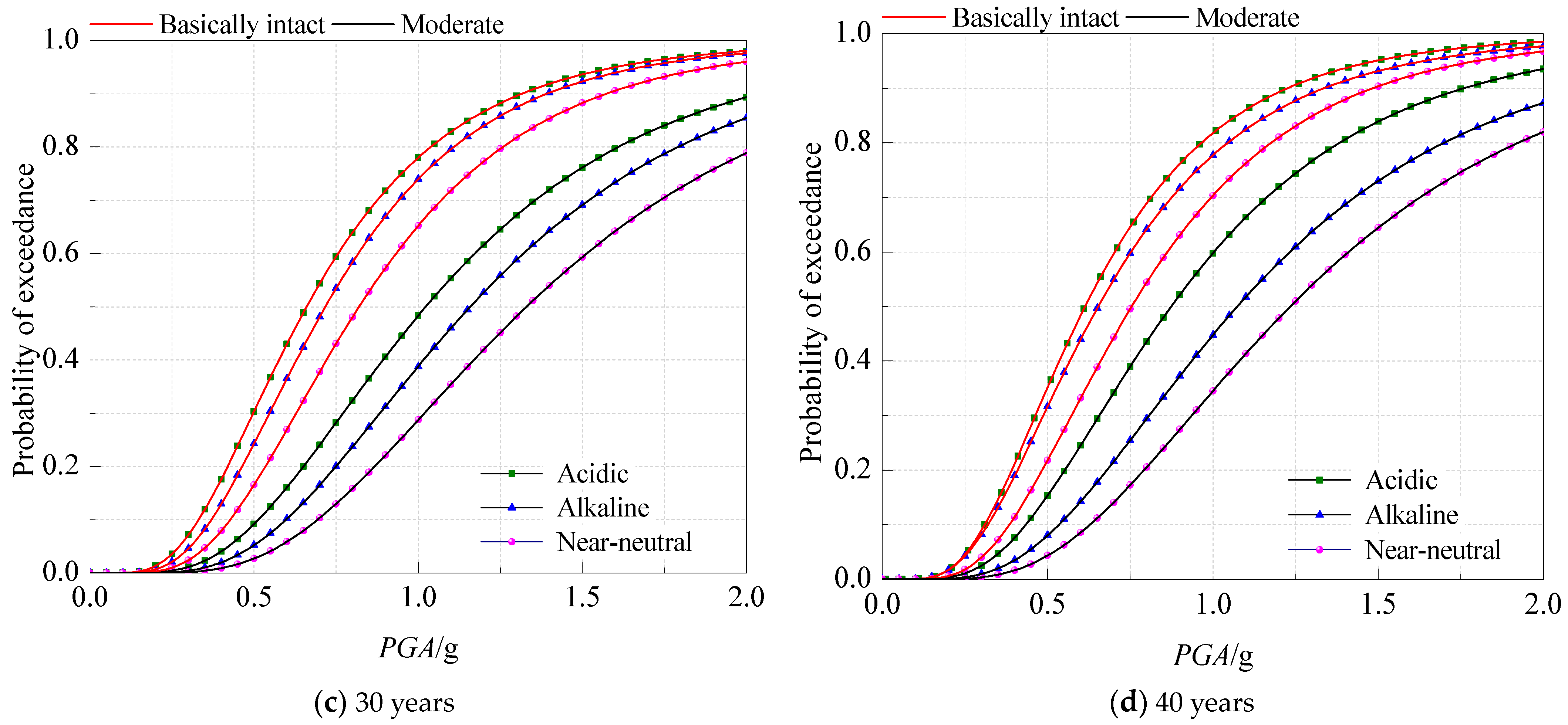
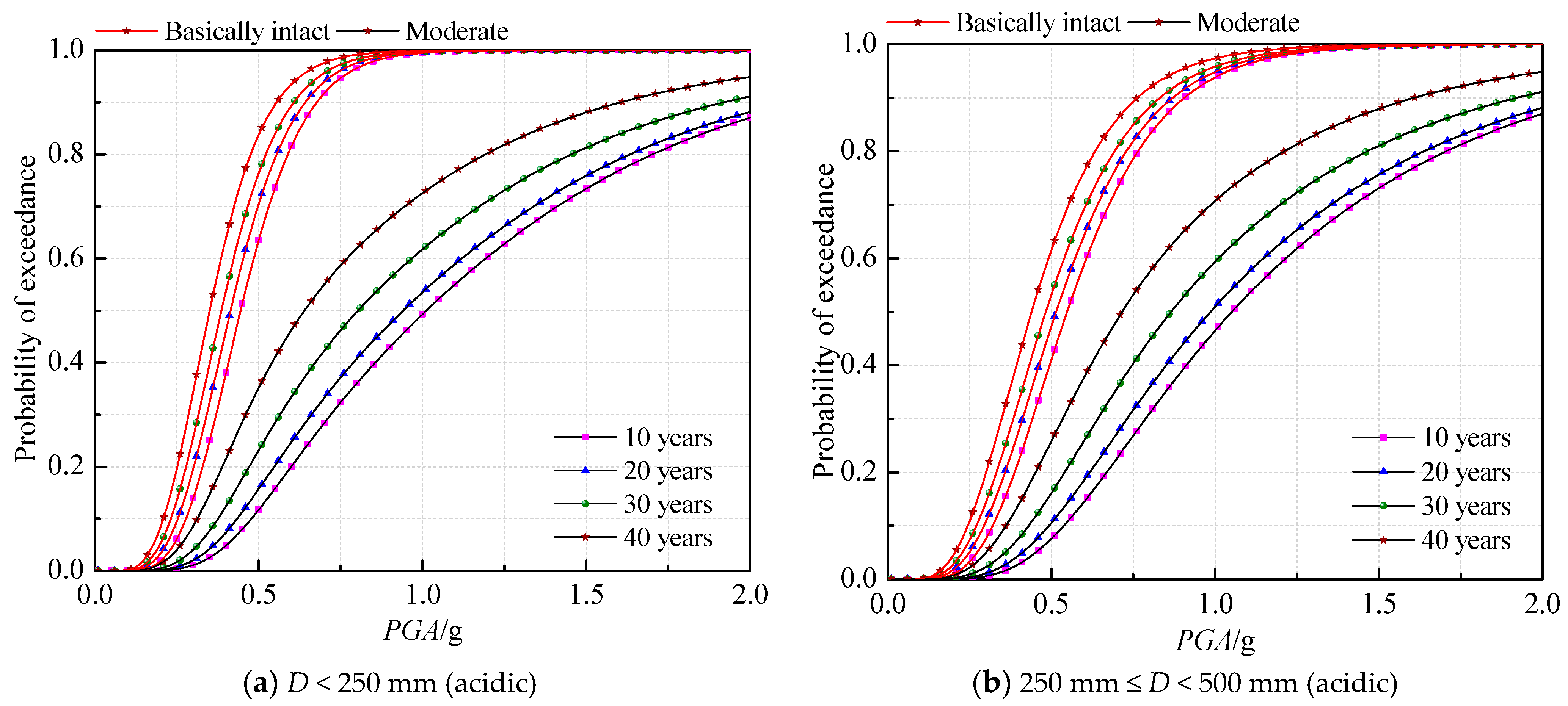
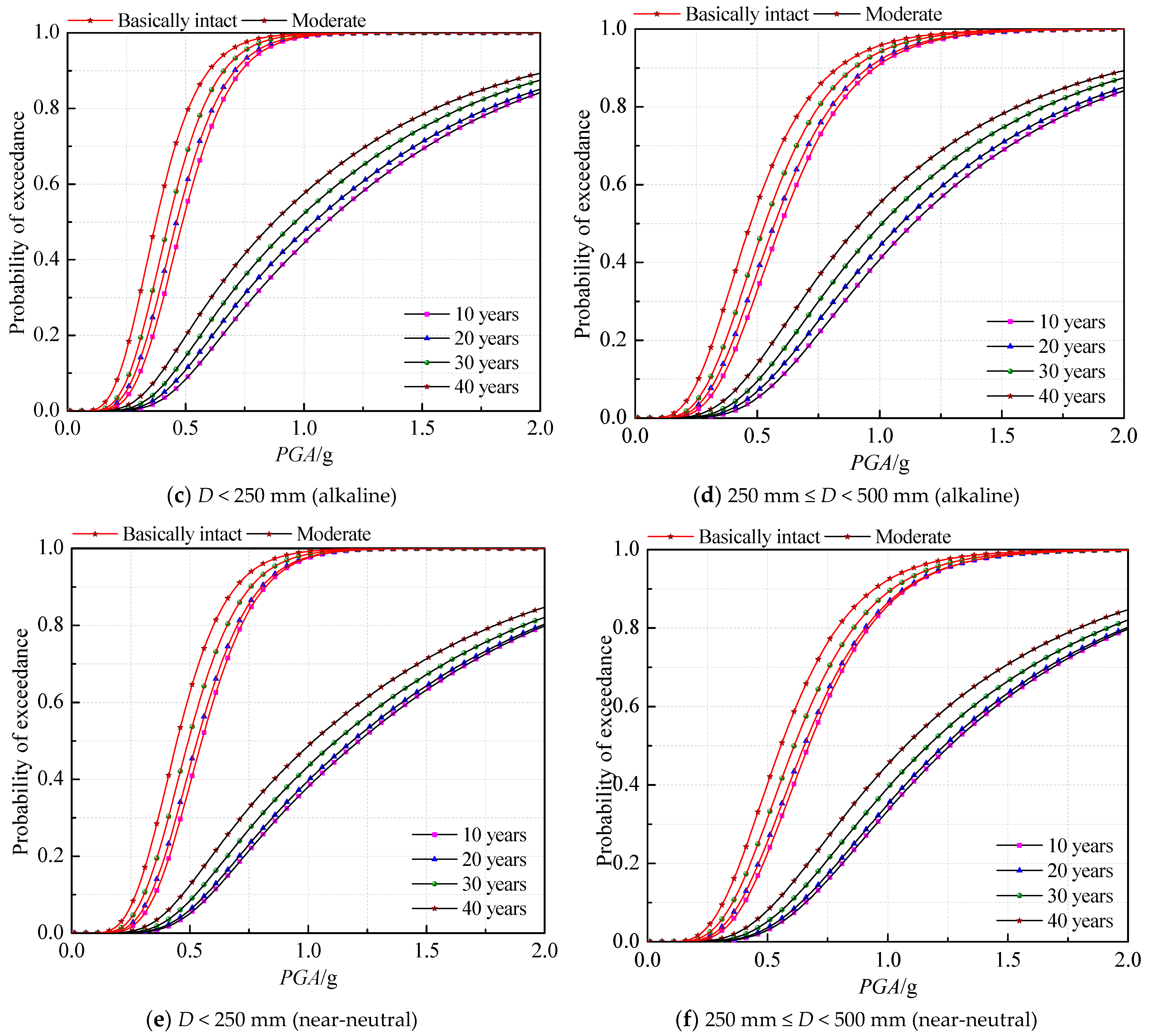
2.2. Seismic Fragility of Pipelines

Earthquake vulnerability analysis predicts the likelihood of failure in structures subjected to varying levels of seismic activity. This analysis quantitatively assesses the seismic performance of engineering structures, illustrating the correlation between ground shaking intensity and structural damage on a macroscopic scale. Seismic vulnerability analysis methodologies encompass empirical methods derived from seismic data [40], analytical methods based on static and dynamic analyses of structural models [41], and approaches grounded in expert empirical judgment [42]. Notably, the analytical seismic vulnerability method typically employs a lognormal cumulative distribution function for its expression:

$$F_R(x)=P[D\ge C|IM=x]=\Phi \left[\frac{\ln x-\ln m}{\beta }\right]$$

(6)

where the term F_R(x) represents the seismic vulnerability function, wherein D denotes earthquake demand, and C represents seismic capability. IM signifies the ground motion intensity parameter, m is defined as the median value of the seismic vulnerability function, and β represents the logarithmic standard deviation of the seismic vulnerability function. Considering the assumption that both structural seismic demand (D) and seismic capacity (C) follow a normal distribution, and considering the uncertainty associated with the structural vulnerability function, this leads to the derivation of the structural analytical seismic vulnerability model, as follows:

$$F_R(x)=\Phi \left[\frac{\ln (m_{D|IM})-\ln (m_{\mathrm{C}})}{\sqrt{{\beta }_{D|IM}^2+{\beta }_{\mathrm{C}}^2+{\beta }_{\mathrm{M}}^2}}\right]$$

(7)

where m_D|IM and m_C are the median values of structural seismic demand and seismic capacity, respectively, and β_D|IM, β_C, and β_M are the quantified values of structural seismic demand uncertainty, seismic capacity uncertainty, and modeling uncertainty, respectively.

This study integrated the established relationship between steel’s mechanical property indices and service age under varying soil corrosion environments, as detailed in Section 2.1, utilizing peak ground acceleration (PGA) and maximum equivalent force (ρ_max) as indices for ground vibration strength and structural seismic response, respectively. In establishing the finite element model of buried pipeline, this study choses the shell-equivalent spring model, using the shell unit to simulate the pipe body, while simplifying the soil body into uniform elastic–plastic springs along the axial, vertical, and transverse directions, which are connected to the nodes of each finite element to simulate the constraints on the buried pipeline in all directions of the soil body [43], and introducing the equivalent boundary spring [44] at the end of the pipeline to consider the influence of the pipeline segments outside the model. Seismic fragility curves for welded continuous steel pipes were developed across various service environments (acidic, near-neutral, and alkaline), different service ages (10, 20, 30, and 40 years), and different pipe diameters (<250 mm, ≥250 mm to <500 mm, and ≥500 mm) based on analytical vulnerability methods, as illustrated in Figure 1 and Figure 2. It is important to note that the term “service age” specifically refers to the duration of pipe usage following the onset of corrosion. The seismic fragility curves of buried pipelines enabled the determination of the likelihood that the pipelines would remain basically intact, suffer moderate damage, or experience severe damage under various seismic impacts.

Upon examining the seismic fragility curves of pipelines across various soil corrosion environments and service ages depicted in Figure 1, it was observed that significant variances were evident in the damage probability of pipelines across distinct soil corrosion environments and damage states, with the probability of damage escalating as the service age increased. The differing corrosion mechanisms and rates in various soil corrosion environments for buried steel pipes led to disparities in the rates of degradation for both mechanical properties and SP. As the service age advanced, the degradation of pipeline SP progressively worsened, culminating in a continuous increase in the probability of pipeline damage.

Upon analyzing the seismic fragility curves of buried pipelines with varying diameters in distinct soil corrosion environments, as depicted in Figure 2, it was observed that under identical seismic intensities and soil corrosion conditions, the diameter of the pipe significantly influenced the seismic response of buried pipelines, with smaller diameters exhibiting a higher likelihood of sustaining damage. This was attributed to the reduced stiffness in pipes with smaller diameters, resulting in inferior seismic performance compared to those with larger diameters. Additionally, an increase in service age and soil corrosivity led to more pronounced degradation of both the mechanical and seismic properties of the pipeline, consequently elevating the damage probability. Generally, steel pipes exhibited superior seismic performance, which varied significantly with the pipe diameter, service age, and soil corrosion conditions.

2.3. Hydraulic Analysis Model

Utilizing the probabilities associated with three damage states of buried pipelines, a stochastic simulation method can be applied to ascertain the specific damage states of the pipelines. Should a water supply pipe be in either a moderately damaged state or a severely damaged state, a virtual leakage or breakage point is introduced to the respective pipe, thereby generating a new WDS topology. Subsequently, the hydraulic equilibrium equation for the WDS post-earthquake is formulated through the solution of node equations, and this equation is resolved employing the Newton–Raphson iterative method [45]:

$$F(H)={AC}_{\mathrm{W}}{\left(A^{T}H\right)}^{\alpha }-Q_{\mathrm{N}}=0$$

(8)

where H is the vector of node hydraulic pressure (m), A is the correlation matrix of the damaged WDS, C_w is the vector of pipe roughness coefficients of the WDS, A^T is the transpose of matrix A, and Q_N is the vector of node flows (m³/s). Among them, the flow rate at the leakage point is calculated using the pipe leakage model based on the outflow orifice [46], and the flow rate at the pipe breakage point is calculated using the virtual reservoir model proposed by Shi [47]. Furthermore, the pressure-driven analysis (PDA) method has been widely used in the post-earthquake hydraulic simulation of WDSs to avoid negative pressure [48,49]. In this study, the node demand and pressure relationship proposed by Gupta and Bhave [50] was used:

$$Q_i=\{\begin{array}{cc}0& H_i\le H_i^{\min }\\ Q_i^{\mathrm{req}}{\left(\frac{H_i-H_i^{\min }}{H_i^{\mathrm{des}}-H_i^{\min }}\right)}^{1/n}& H_i^{\min }<H_i<H_i^{\mathrm{des}}\\ Q_i^{\mathrm{req}}& H_i\ge H_i^{\mathrm{des}}\end{array}$$

(9)

where Q_i and Q_i^req are the available water flows (m³/s) and the original water demand flows (m³/s) at node i, respectively. H_i is the actual water pressure (m) at node i, H_i^min is the minimal water pressure (m) at which the node i can supply water flows, and H_i^des is the water pressure (m) required to fulfill the original demand flows, while n is an empirical coefficient, generally taken as 1.5~2.

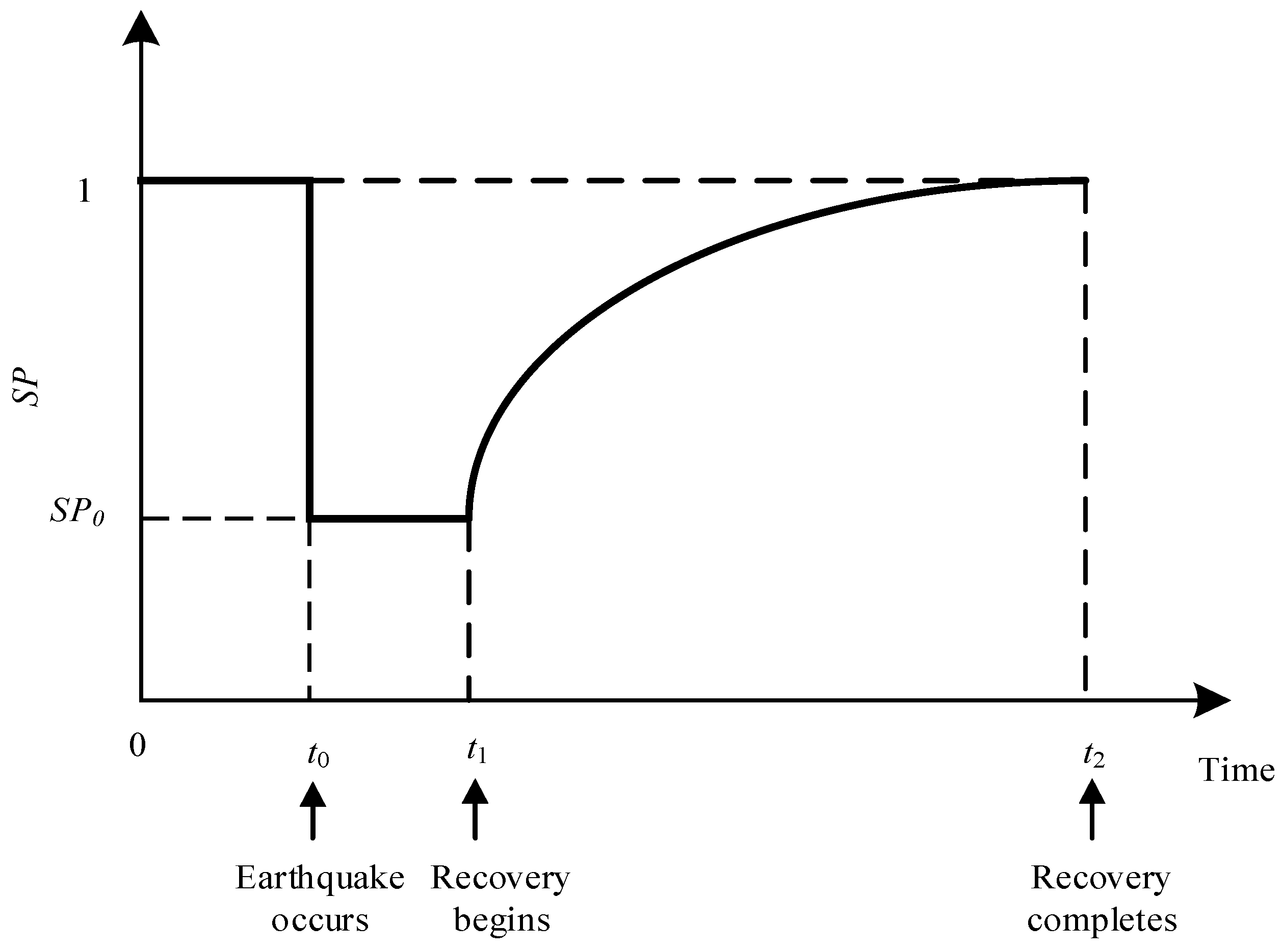
2.4. Seismic Resilience Assessment Method for WDS

To analyze the SR of the WDS, it was essential to first define the system performance indicator. This study employed the demand-based SP for WDS, as proposed by Liu et al. [13]. The entire process of the WDS, from experiencing an earthquake to the completion of gradual restoration, is depicted in Figure 3. At t₀, an earthquake occurred, causing the SP to drop to a low level (SP₀), which persisted until recovery activities commenced at t₁. The period from t₁ to t₂ represents the recovery stage, and by t₂, SP gradually recovered to its pre-earthquake level.

This paper employed the weighted average of user node satisfaction to define the WDS’s overall satisfaction and serve as an SP indicator. The ratio of the area enclosed by the WDS performance curve and the time axis to the control time served as the SR metric, with the specific calculation formula provided below:

$$SR=\frac{1}{t_2-t_0}{\displaystyle {\int }_{t_0}^{t_2}SP(t)dt}$$

(10)

where SP(t) denotes the overall satisfaction of the WDS at time t (h), and its mathematical expression is:

$$SP(t)={\displaystyle \sum _{i=1}^n{w}_i\left(t\right)\cdot NS{D}_i}(t)$$

(11)

where w_i(t) is the weight coefficient of node i at time t, and at any t, Σw_i(t) = 1, n is the number of nodes, and NSD_i(t) is the satisfaction degree of node i at time t, which is given by [23] as:

$$NS{D}_i(t)=\{\begin{array}{cc}1& H_i\left(t\right)\ge H_i^{\mathrm{des}}\left(t\right)\\ \frac{H_i\left(t\right)}{H_i^{\mathrm{des}}\left(t\right)}& H_i\left(t\right)<H_i^{\mathrm{des}}\left(t\right)\end{array}$$

(12)

where H_i(t) and H_i^des(t) are the post-earthquake free water pressure (m) and demand water pressure (m) at node i at time t, respectively.

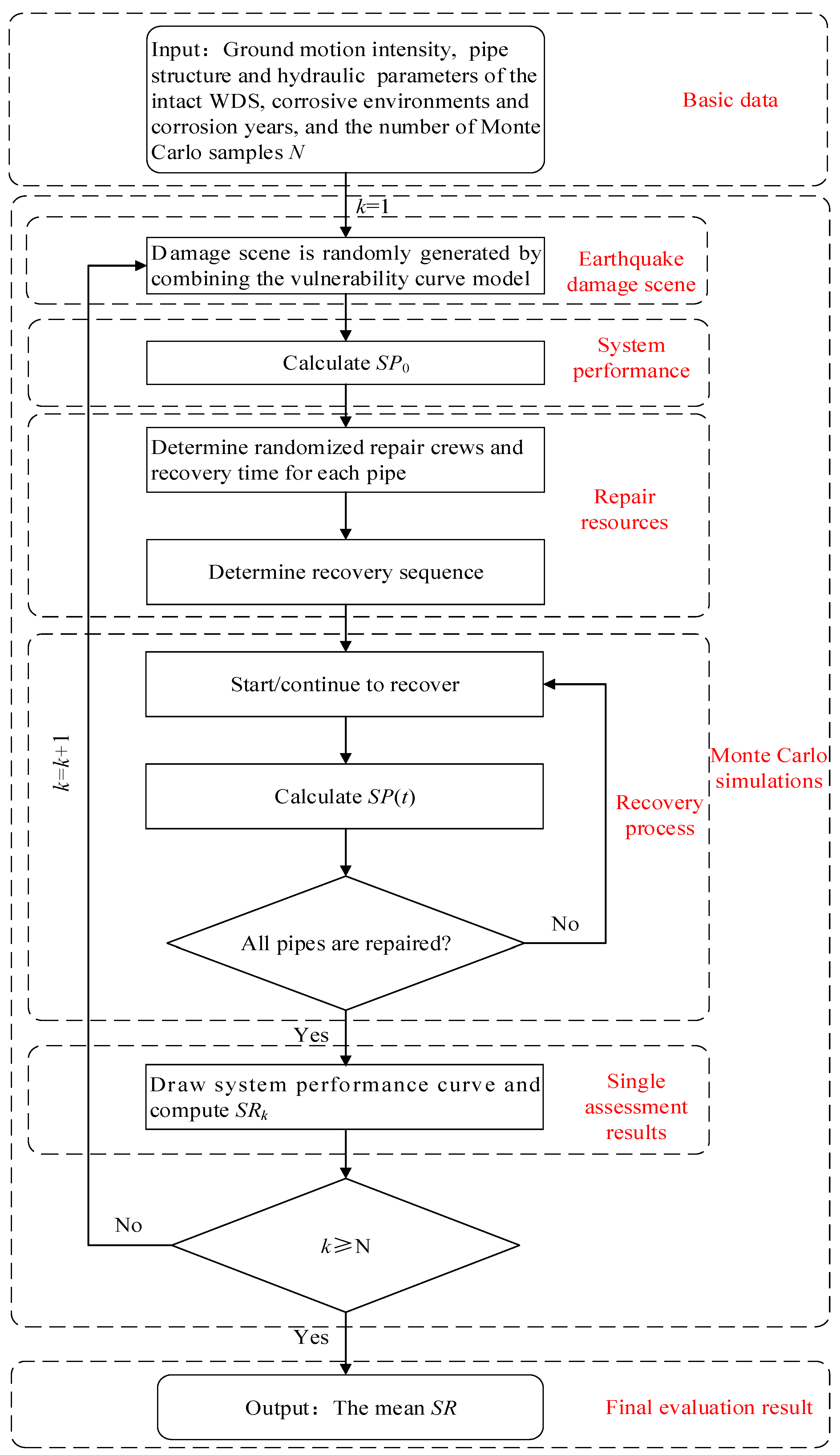
2.5. Monte Carlo Simulation

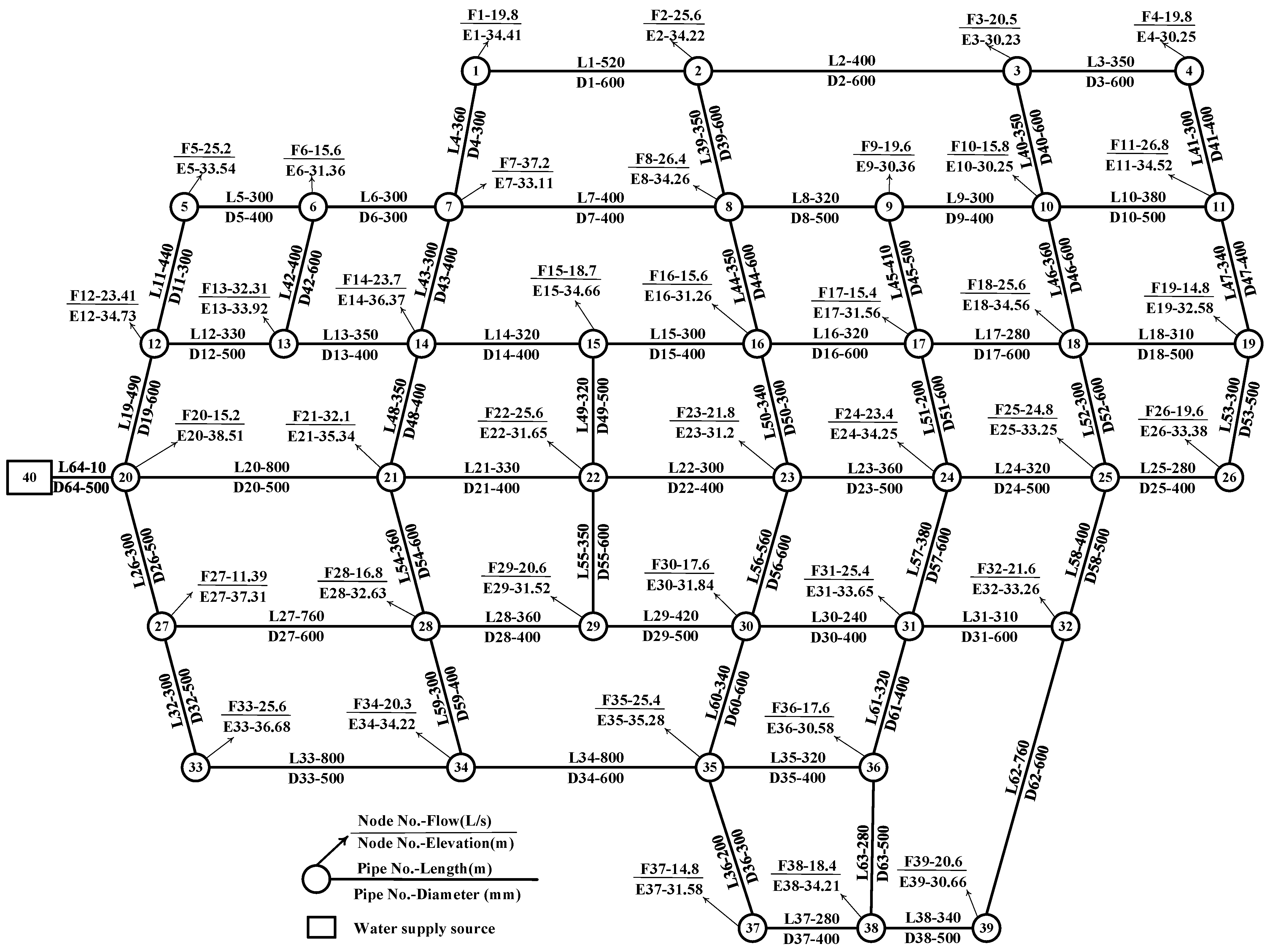
Since earthquake-induced pipeline damage is expressed in terms of the earthquake damage probability, the state of the pipeline after a seismic event is a random variable. Meanwhile, this study assumed that the repair sequence and repair time of the pipeline after the earthquake were also random variables. Thus, the Monte Carlo simulation (MCS) method was used to generate the damage samples, repair sequence samples, and repair time samples of pipelines, and evaluate the SR of the WDS. If the number of MCS samples was N, then the SR was estimated by the mean value of the results of N samples, and the formula was as follows:

$${\mu }_{SR}=\frac{1}{N}{\displaystyle \sum _{k=1}^{N}S{R}_k}$$

(13)

where SR_k is the post-earthquake SR in the kth MCS sample.

The flowchart for the SR evaluation utilizing these aforementioned models in Section 2.1, Section 2.2, Section 2.3, Section 2.4 and Section 2.5 is shown in Figure 4.

3. Case Study

To compare the SR of WDS with varying degrees of corrosion, we validated the theoretical model presented in Section 2 using the WDS case described in [51]. Figure 5 illustrates the layout of the WDS, comprising 40 nodes and 64 pipelines. The water supply source, node 40, maintained a constant water level of 60 m. Assuming all network pipes were welded steel, Figure 5 details their lengths, diameters, node elevations, and pre-seismic flow rates. The WDS site was classified as Class II, with a seismic fortification grade of VIII. Subsequently, the SR of WDS was analyzed under 36 different scenarios, encompassing various seismic intensities (frequent, design, and rare earthquakes), soil environments (acidic, alkaline, and near-neutral), and corrosion ages (10, 20, 30, and 40 years).

3.1. Results of Hydraulic Analysis under Different Working Conditions

In the PDA approach for hydraulic simulations, the parameters were set as H_i^min = 0 m and H_i^des = 15 m. Pipeline head losses were calculated using the Hazen–Williams formula. The hydraulic imbalance equation was solved using the Newton–Raphson method, with iteration accuracy set at 0.0001. For each of the 36 different working conditions previously outlined, 1000 simulations were conducted. The SP of the WDS was recorded for each simulation under varying damage states. Figure 6 displays the residual SP of the WDS across different seismic damage scenarios.

As can be seen in Figure 6, the post-earthquake SP of the WDSs with the four service ages in the three environments remained unaffected under frequent earthquakes, maintaining pre-earthquake service levels. Under fortification earthquakes, the decrease in post-earthquake SP for WDSs was negligible. Under the influence of rare earthquakes, the post-earthquake SP of the WDSs in near-neutral environments was minimally impacted. Specifically, the SP values for WDSs of four different service ages were 0.9833, 0.97722, 0.96062, and 0.92382, respectively. In alkaline environments, the SP for WDSs of the same four service ages decreased by 3.9%, 6.2%, 9.9%, and 17.1%, respectively, compared to their pre-seismic performance. In acidic environments, the decrease in SP was more pronounced, with reductions of 10.5%, 17.0%, 17.5%, and 32.0% for the four service ages, respectively. The SP of the WDSs with a service age of 40 years in an alkaline environment was comparable to those with service ages of 20 and 30 years in an acidic environment. However, the SP for WDSs at 40 years in a near-neutral environment exceeded that of WDSs at 30 years in an alkaline environment and 10 years in an acidic environment. This indicates that the effect of the soil’s corrosive environment significantly outweighs the impact of service age on the SP of WDSs for this seismic intensity. At a service age of 40 years, the SP degradation of the WDSs in an acidic environment was 2 and 4 times greater than that of the pipeline in an alkaline environment and a near-neutral environment, respectively. The maximum relative difference in SP degradation across various service ages was 30.3%. In order to further investigate the effects of soil conditions and service ages on the SP of WDSs, the significance of the differences in the SP of WDSs with different soil conditions and service ages under the effects of fortified earthquakes and rare earthquakes was analyzed by using one-way factorial analysis of variance (ANOVA). The analysis results showed that, under the effects of fortification earthquakes, the soil conditions, service ages, and the combined effects of soil conditions and service ages all had a significant effect on the seismic performance, and the corresponding significance was less than 0.001. Under the effects of rare earthquakes, the same conclusion could be reached with the corresponding significance of 0.000, which was less than the set significance level of 0.05. Overall, the SP of WDSs in the four environments decreased with the increasing seismic intensity and service age. At the same seismic intensity, the acidic environment had the most substantial impact on SP, followed by the alkaline environment, with the near-neutral environment having the least impact.

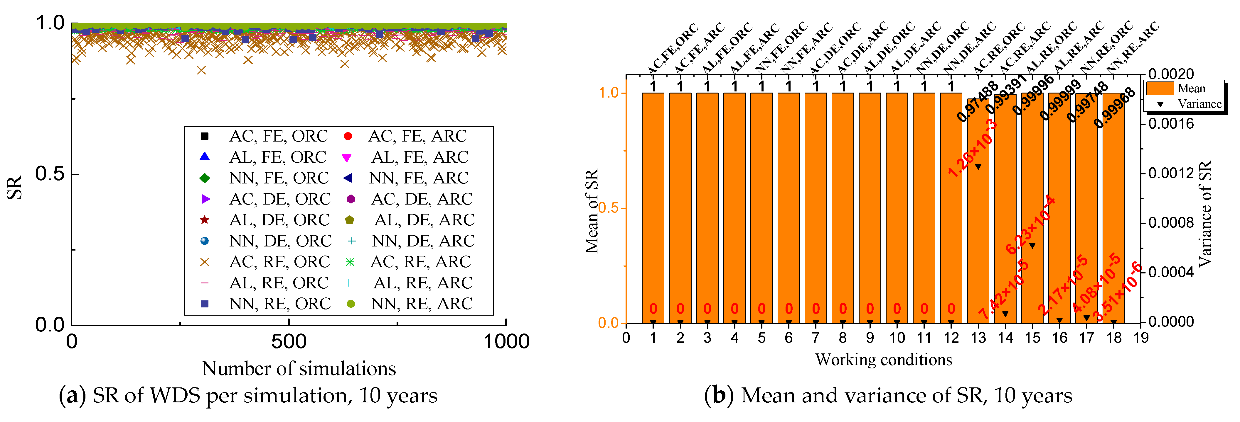
3.2. Seismic Resilience Evaluation Results

The assessment of the resilience of WDSs needs to take into account the network repair process following an earthquake [52]. This study focused solely on two scenarios: the longest and shortest repair times, employing either a single repair crew fixing broken pipes sequentially or a repair crew assigned to each damaged pipe concurrently. Then, the range of SR of WDS was calculated based on these approaches. The time taken by each repair team to repair the corresponding broken pipe was determined using a random sampling simulation. Repair times for each scenario were estimated using a random sampling simulation, where the time to repair a leaky pipe by a full repair crew was modeled by a normal distribution with a mean of 6 h and a variance of 3 h, and the time to repair a broken pipe followed a normal distribution with a mean of 12 h and a variance of 6 h [53]. Utilizing the Monte Carlo method, 1000 simulations were conducted to model the recovery process of the earthquake-damaged pipe network (illustrated in Figure 7, Figure 8, Figure 9 and Figure 10). Due to spatial constraints, this paper only presents the recovery curves for WDSs with service ages of 30 and 40 years under both rehabilitation strategies. To compare the SR of WDSs under various operational conditions, this study examined the SR at the 180th hour post-earthquake (equivalent to 15 days, assuming 12 h of repair work per day by each crew), as shown in Figure 11.

From Figure 7, Figure 8, Figure 9 and Figure 10, it was evident that the SP of the WDS remained at pre-earthquake levels throughout the restoration process for service ages of 30 and 40 years under frequent earthquakes. Under fortification earthquake conditions, the average total repair times for damaged pipes in acidic, alkaline, and near-neutral environments were 8.4 h, 4.0 h, and 1.6 h, respectively, for a service age of 30 years, and 14.4 h, 10.0 h, and 3.4 h for a service age of 40 years. When employing a single repair team under rare earthquake effects, the mean total repair times across the three environments were 116.2 h, 83.2 h, and 49.2 h for a service age of 30 years, and 152.6 h, 118.0 h, and 72.3 h for a service age of 40 years, respectively. As seismic intensity and service age increased, the incidence of pipe failures rose, and the complete repair time correspondingly lengthened, with acidic environments requiring the most time. Conversely, employing multiple repair crews for simultaneous repairs can restore the WDS within 20 h, irrespective of the environment or earthquake intensity, highlighting the critical role of maintaining ample emergency repair resources.

Figure 11 reveals that the SR of the WDS across all four service ages in the three environments remained at 100% under frequent earthquakes, irrespective of the rehabilitation strategy employed. Under the action of the fortification earthquake, although a few pipelines were broken, they were quickly repaired, and the SR of the WDS in the three environments was still 100% when the service age was less than 20 years. Beyond 20 years, the SR experienced a slight decline, though it remained near 100%. Under rare earthquake conditions, pipeline damage occurred in all three soil environments for service ages of 10 and 20 years. In the acidic environment, the incidence of pipeline damages was notably higher compared to other conditions. When a single repair crew was deployed, the average values of the SR of the WDS were 0.9749 and 0.9656, respectively. However, assigning a dedicated team to address each damage pipe simultaneously resulted in improved average SR values of 0.9939 and 0.9932, respectively. Conversely, in alkaline and near-neutral soil environments, the SR of the WDSs was higher under both rehabilitation strategies, attributed to the relatively lower occurrence of pipeline damages. When the service age of the WDS was 30 years, the average SR in acidic and alkaline environments was 0.940 and 0.974, respectively, with a single repair crew deployed. When a team was assigned to each failure pipe, the average SR improved to 0.991 and 0.995, respectively. In the near-neutral environment, employing the two repair strategies resulted in SR values of 0.993 and 0.998, respectively. When the service age of the WDS was 40 years, the SR in the acidic environment declined significantly, by 16.2%, with only one repair crew. However, assigning a crew to each damage pipe elevated the SR to 98.2%, thereby exceeding the SR observed in the alkaline environment under the one repair crew approach. The analysis illustrated the significant impact of emergency resource allocation on the SR of WDSs. With constant seismic intensity, the greatest variation in SR values due to different service ages in an acidic environment reached 16.3%. Across all three environments, the maximal discrepancy in SR values was observed to be 19.3%.

For identical service ages and soil conditions, the SR of the WDS progressively diminished as seismic intensity escalated. With equal service ages and high seismic activity, the SR was most adversely affected in acidic soil environments, whereas it exhibited the highest resilience in nearly neutral soil conditions. Additionally, under consistent soil conditions and significant seismic events, the SR systematically declined with the increasing service age. The deployment of multiple repair teams significantly boosted the SR across all scenarios. Since the WDS pipelines were exclusively composed of steel, the overall SP was robust, ensuring a high SR even during rare earthquakes.

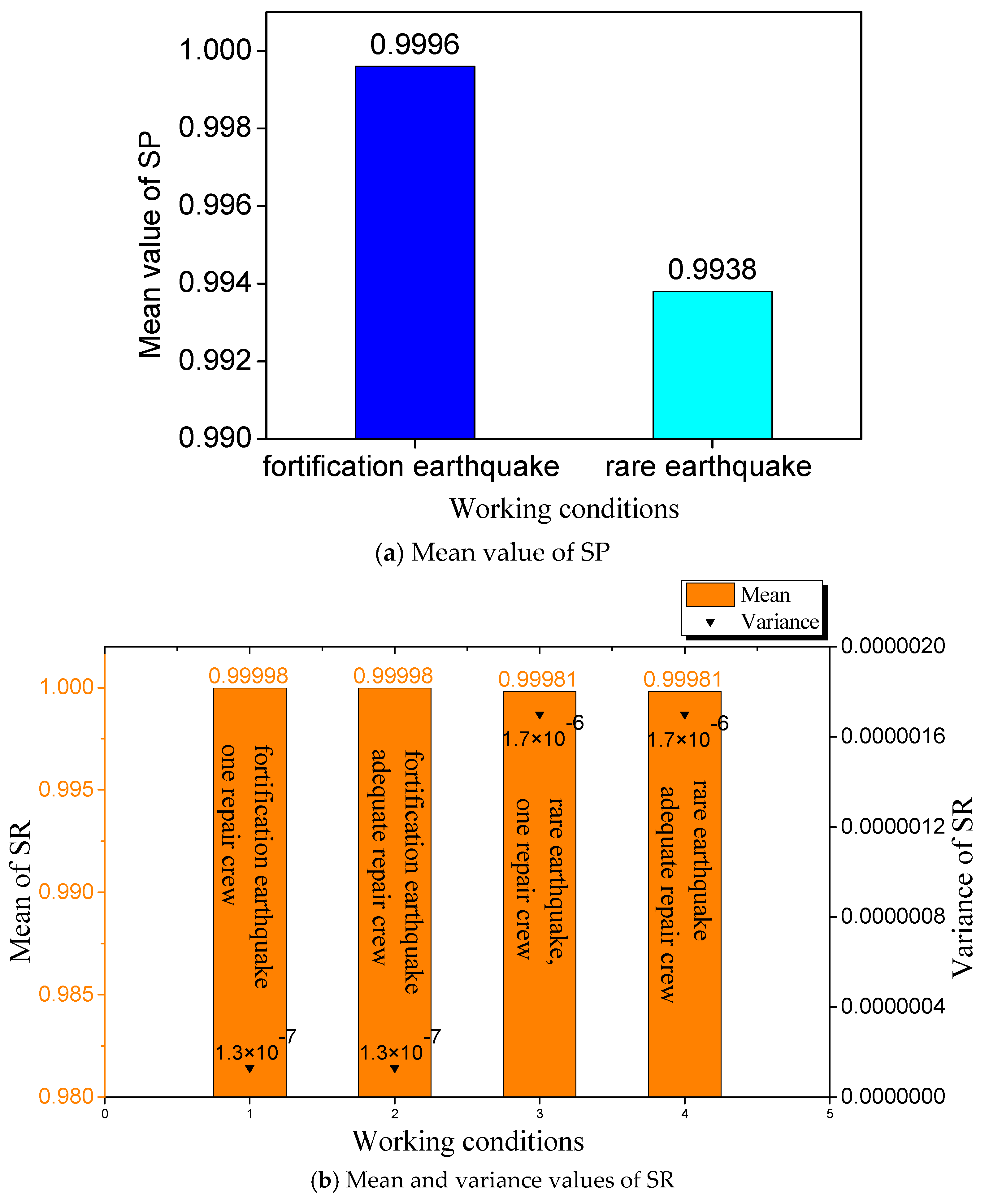
3.3. Results of Seismic Resilience Assessment Based on Empirical Data

To further scrutinize the impact of corrosive environments and service age on the SR of WDS, this study compared the results of calculations presented in Section 3.2 with those derived from a SR assessment based on historical empirical data. It is imperative to note that the empirical approach typically treats post-earthquake pipeline failures as stochastic events. Consequently, earthquake-induced damages are assumed to manifest randomly and independently along the pipeline, adhering to a Poisson distribution. Subsequently, the probability of encountering the three failure states was computed using Equation (14):

$$\{\begin{array}{l}{P}_{f3}=1-e^{-0.15·R_f·L}\\ P_{f2}=1-e^{-0.85·R_f·L}\\ P_{f1}=1-P_{f2}-P_{f3}\end{array}$$

(14)

where P_f1, P_f2, and P_f3 denote the probability of the pipeline being basically intact, moderately damaged, and severely damaged, respectively, and L is the length (km) of the pipeline. R_f is the pipe repair rate, expressed as repairs/km. This paper adopted the formula for calculating the R_f of water supply pipelines provided by the Japan Water Works Association [54], which is expressed as follows:

R_f = C_d·C_p·C_g·C_l·R₀

(15)

R₀ = 2.88·10⁻⁶·(PGA-100)^1.97

(16)

where C_d, C_p, C_g, and C_l represent the correction factors for the pipe diameter, pipe material, topography, and liquefaction, respectively. R₀ is the standard pipeline repair rate.

For the earthquake scenarios of fortification (0.2 g) and rare (0.4 g) intensities, this study calculated the three-state damage probability for each pipeline within the network using Equation (14). Following this, 1000 simulations were conducted using the SR evaluation method outlined in Section 2, and the results of SR are shown in Figure 12.

As illustrated in Figure 12, the post-earthquake SP of the WDS under fortification seismic action (0.2 g) was assessed at 0.9996 when using empirical data. This SP surpassed that observed in both acidic and alkaline soil conditions under equivalent seismic intensity. However, it was slightly lower than the SP in near-neutral conditions for service ages of 10 and 20 years, comparable to a 30-year service age, and marginally higher than a 40-year service age. The average SP for the WDS across 12 conditions under fortification earthquakes stood at 0.9968, generally below the simulation outcomes based on empirical data. Under rare seismic events (0.4 g), the WDS post-earthquake SP was 0.9938, exceeding that under all other conditions for the same seismic intensity. The greatest disparity, at 46%, was observed against the SP of the WDS in an acidic environment with a 40-year service age. The average SP for 12 conditions under rare earthquakes was 0.892, showing an 11% variance from empirically based calculations, indicating a generally high SP of the WDS when derived from empirical data.

The SR value of the WDS under fortification seismic action was calculated at 0.99998 based on empirical data, consistent across both types of rehabilitation. With minimal pipe damage in each simulation, the SP of the WDS remained at 100%, allowing for swift repair completion whether by a single team or multiple teams concurrently. The SR values were comparable to those of the WDS in the near-neutral environment with a service age of 30 years under fortification earthquakes and exceeded those of WDSs in the same environments with a 40-year service age. Across all four service ages in the three environments, the average SR of the WDS was 0.99998, aligning with empirical SR assessments. Under rare seismic events, while the number of leaking pipes increased in each simulation, the impact on the SR of the WDSs remained minor, registering at 0.9998 under both repair methods. Although lower than the SR of WDSs in certain conditions, such as alkaline environments with a service age of 10 years and 20 years under the same seismic intensity, it surpassed the SR of WDSs in other conditions, with differences reaching a maximum of 19%. The average SR for all service ages across the three environments was 0.981, slightly lower than empirical SR assessments. Despite this, the disparity between analytical and empirical SR results was not significant, primarily due to the robust SP of buried steel pipes. Overall, empirical methods tended to slightly overestimate the SR of the WDS.

4. Conclusions

In this research, a novel assessment method for both SP and SR of WDS was introduced, accounting for factors such as corrosive environmental conditions and the service age of buried pipelines. The effectiveness of the proposed method was tested through case studies across 72 distinct scenarios, which included variations in corrosive environments, pipeline service ages, earthquake intensities, and repair crew assignments. These scenarios were further compared against SR values derived from historical empirical data. Key findings from the study are summarized below.

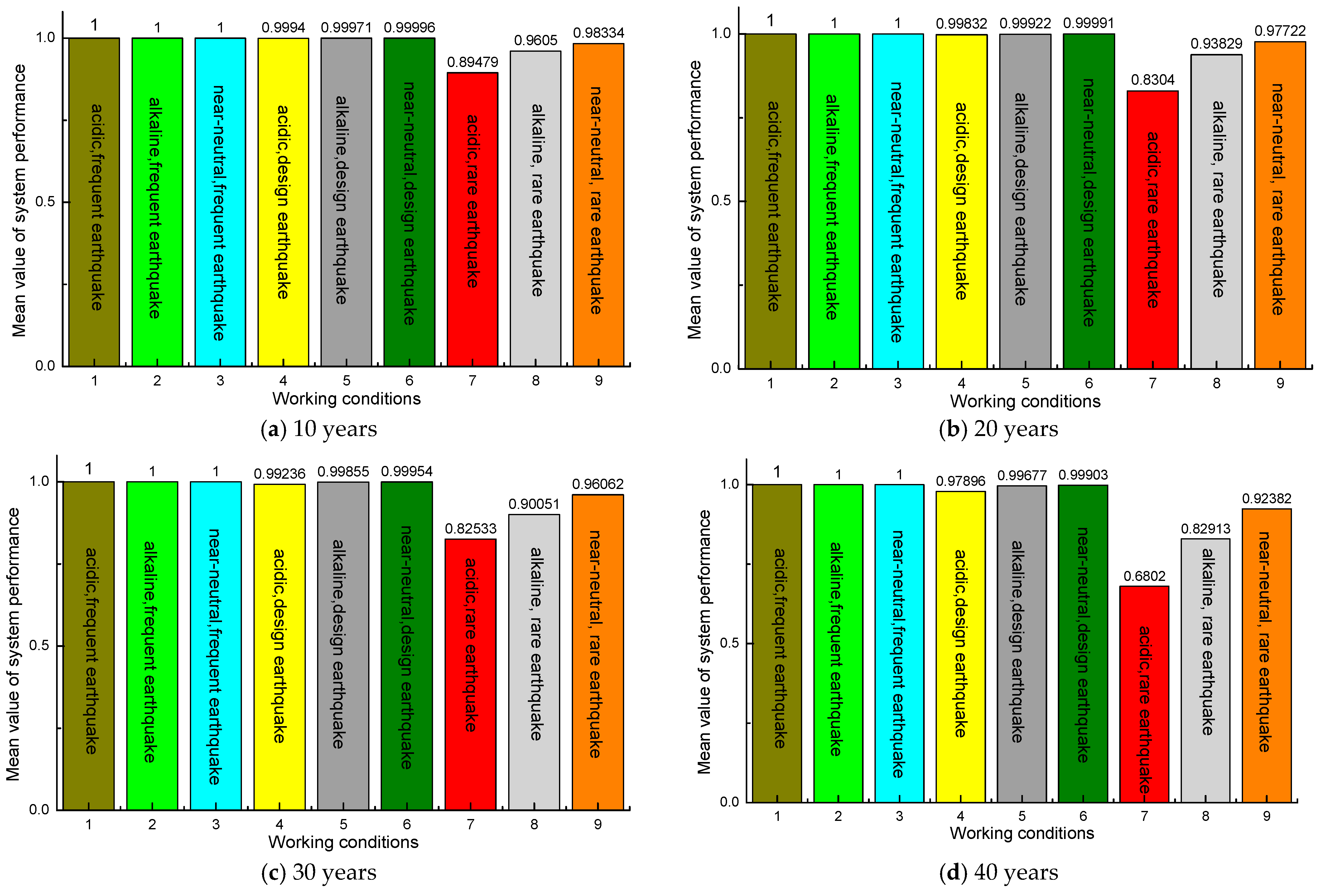
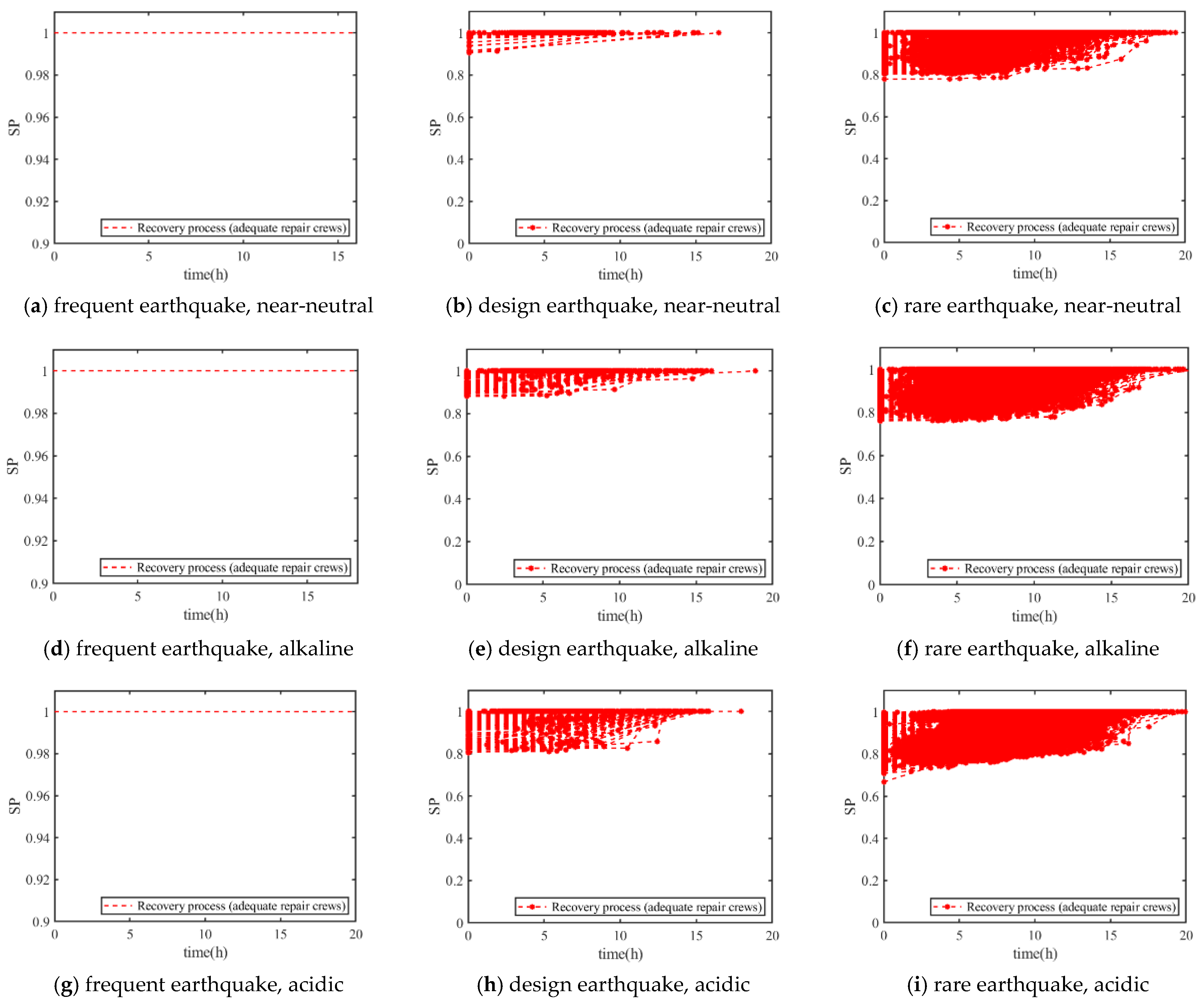
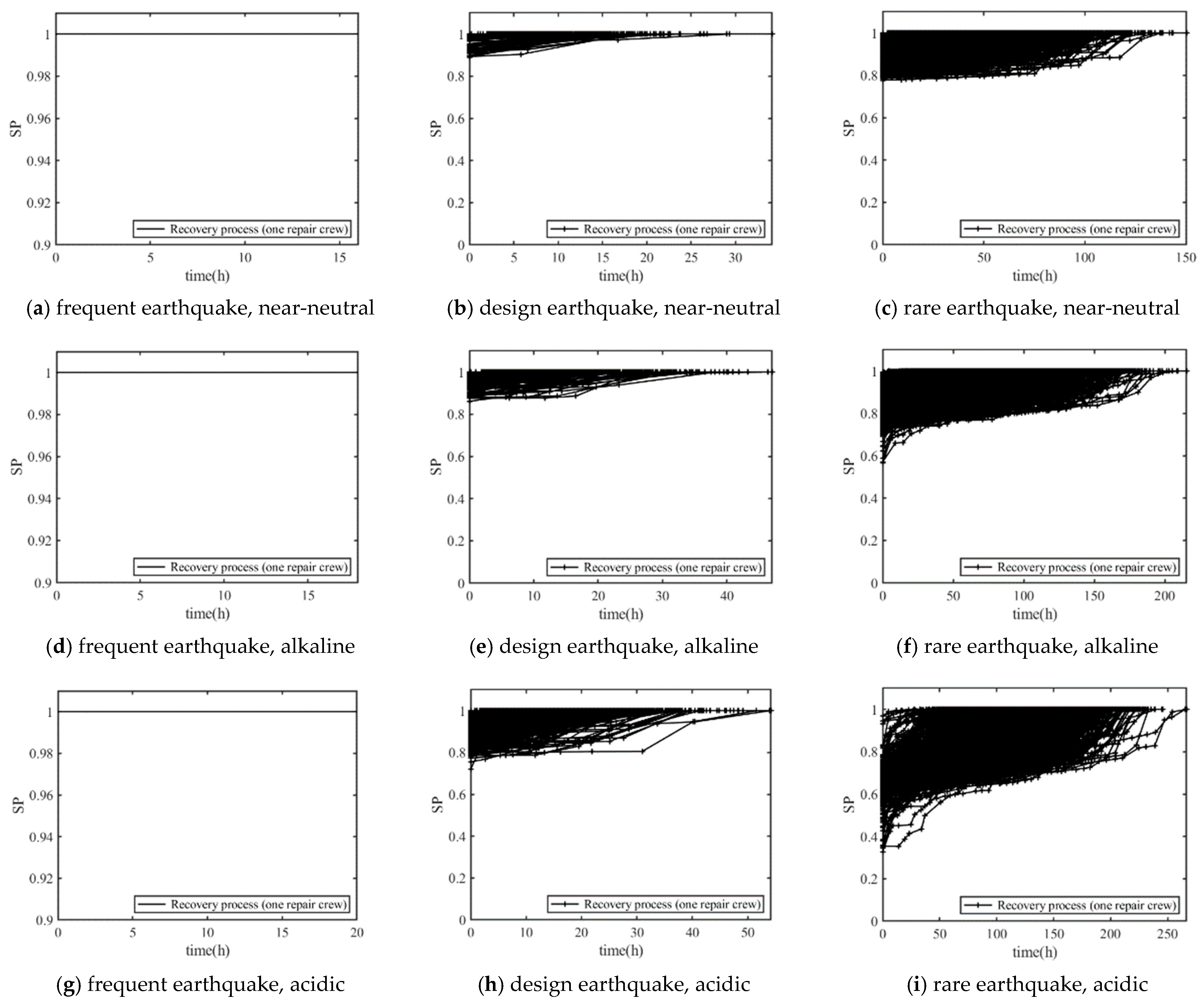
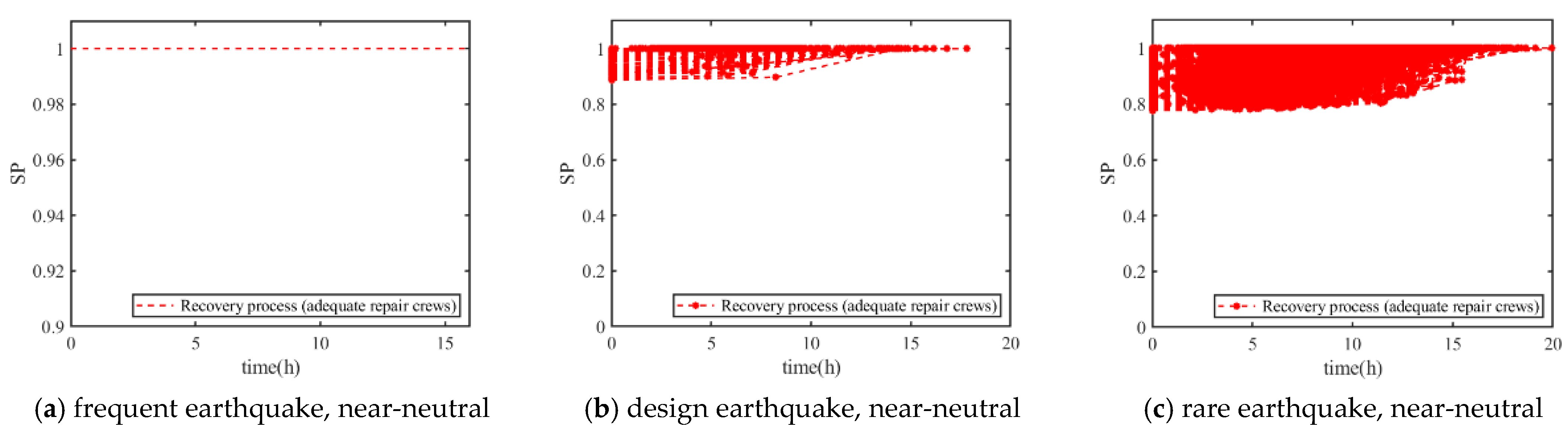
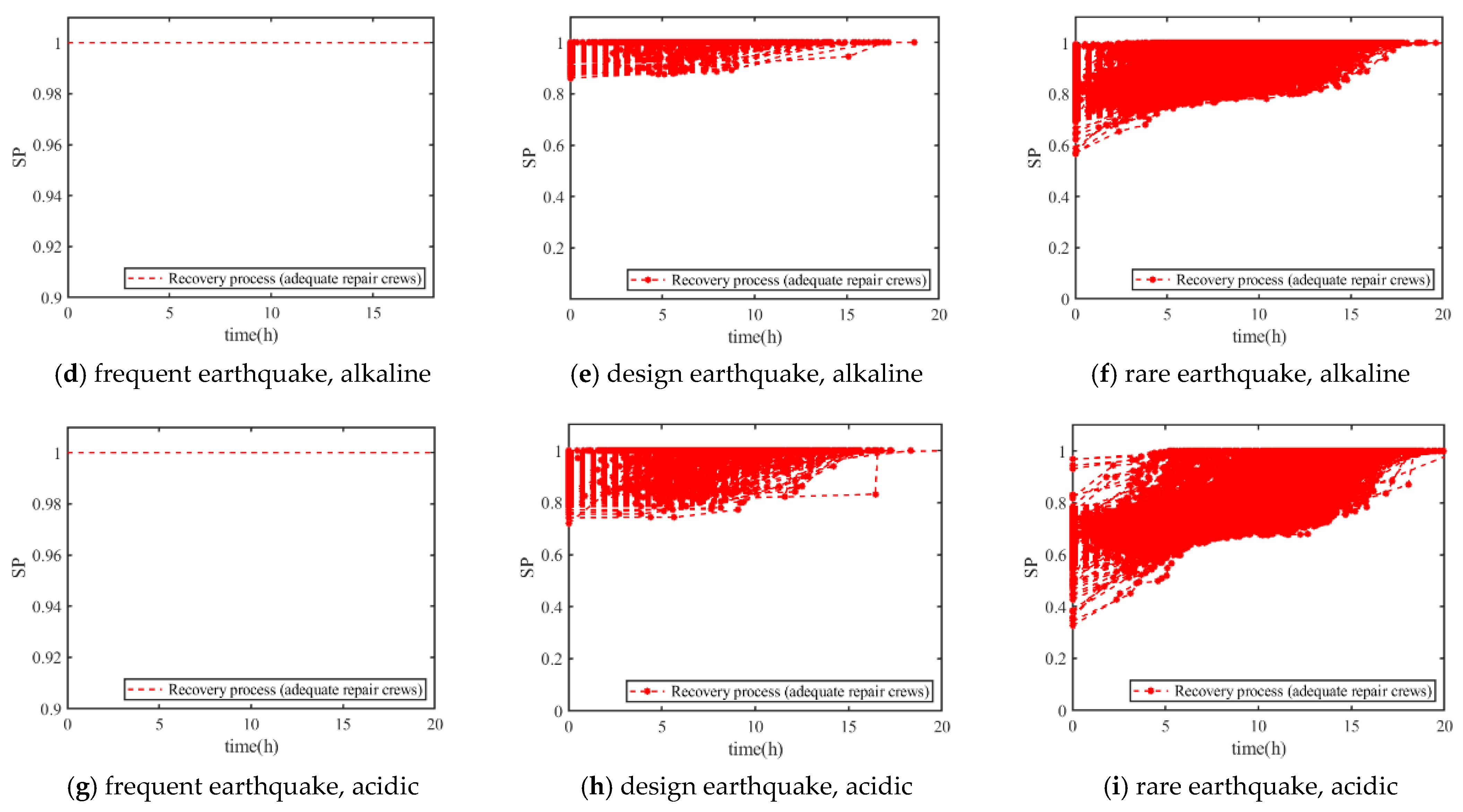
• The simulation results indicated that both SP and SR remained at 100% across various service ages and soil conditions when subjected to frequent earthquakes.
• The SP and SR for the four service ages in the three soil environments did not differ significantly under the effects of a fortification earthquake. Compared with the simulation results under frequent earthquakes, there was a slight decrease, but the overall decrease was not significant.
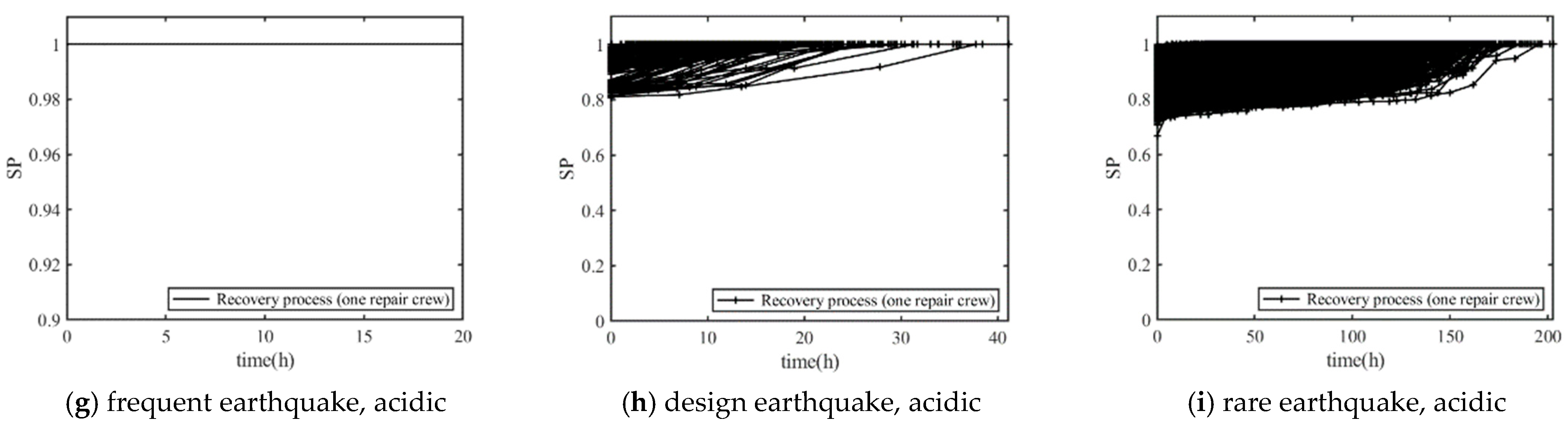
• Under rare earthquake conditions, SP and SR varied significantly, especially in acidic environments where performance notably declined, with the worst recorded SP being 0.68 for pipelines with a service age of 40 years. Despite this, the overall performance across different conditions remained relatively high, with SP values ranging from a minimum of 83.8% to a maximum of 98.2%, and an average SP of 91%. This showed that post-earthquake restoration resources are a key factor in guaranteeing a high level of the SP.
• Holding the service age and soil environment constant, the SR diminished progressively as seismic activity intensified. Under identical service ages and high seismic intensities, the SR was lowest in acidic soil environments and highest in near-neutral soil environments. Considering a constant soil environment and high seismic activity, the SR progressively declined with the advancing service age. The assignment of multiple repair crews universally resulted in a high SR for the WDSs.
• Based on evaluations using empirical data, the SP and SR, when assessed without accounting for variations in soil corrosion conditions and the service age of the pipelines, tended to be estimated on the higher side.

Based on the results of this study, policymakers should focus on pipelines in acidic soil environments, especially those with a long service age, during routine pipeline network maintenance, reinforcement, and identification of damaged pipelines after earthquakes, so as to enhance the SR of WDSs. While this study made some advancements, it solely focused on the SR of corroded steel pipes. Future research is suggested to expand on the SR assessment of other metallic pipelines affected by the soil environment and service age. Additionally, the authors identified that simulating the repair process became significantly time-consuming as the number of broken pipes increased, which is an urgent issue to be addressed in the subsequent research.

References

1. Zhai, C.; Zhao, Y.; Wen, W.; Qin, H.; Xie, L. A novel urban seismic resilience assessment method considering the weighting of post-earthquake loss and recovery time. Int. J. Disaster Risk Reduct. 2023, 84, 103453. [Google Scholar] [CrossRef]
2. Taghizadeh, M.; Mahsuli, M.; Poorzahedy, H. Probabilistic framework for evaluating the seismic resilience of transportation systems during emergency medical response. Reliab. Eng. Syst. Saf. 2023, 236, 109255. [Google Scholar] [CrossRef]
3. Liu, J.; Tian, L.; Yang, M.; Meng, X. Probabilistic framework for seismic resilience assessment of transmission tower-line systems subjected to mainshock-aftershock sequences. Reliab. Eng. Syst. Saf. 2024, 242, 109755. [Google Scholar] [CrossRef]
4. Li, Z.; Lim, H.W.; Li, N.; Long, Y.; Fang, D. Assessing the seismic resilience of a healthcare system: A hybrid modeling. Int. J. Disaster Risk Reduct. 2023, 93, 103730. [Google Scholar] [CrossRef]
5. Liu, W.; Wu, Q.X. Seismic resilience analysis of water distribution networks with multi-components and resilience improvement strategies. J. Seismol. Res. 2023, 46, 271–279. [Google Scholar] [CrossRef]
6. Scawthorn, C. Water Supply in Regard to Fire Following Earthquakes; Pacific Earthquake Engineering Research Center: Berkeley, CA, USA, 2011. [Google Scholar]
7. Miyajima, M. Damage analysis of water supply facilities in the 2011 great east japan earthquake and tsunami. In Proceedings of the 15th World Conference in Earthquake Engineering, Lisbon, Portugal, 24–28 September 2012; pp. 24–28. [Google Scholar]
8. Manyena, S.B. The concept of resilience revisited. Disasters 2006, 30, 433–450. [Google Scholar] [CrossRef] [PubMed]
9. Bruneau, M.; Chang, S.E.; Eguchi, R.T.; Lee, G.C.; O’Rourke, T.D.; Reinhorn, A.M.; Shinozuka, M.; Tierney, K.; Wallace, W.A.; Von Winterfeldt, D. A framework to quantitatively assess and enhance the seismic resilience of communities. Earthq. Spectra 2003, 19, 733–752. [Google Scholar] [CrossRef]
10. Pagano, A.; Giordano, R.; Portoghese, I. A pipe ranking method for water distribution network resilience assessment based on graph-theory metrics aggregated through Bayesian belief networks. Water Resour. Manag. 2022, 36, 5091–5106. [Google Scholar] [CrossRef]
11. Li, W.; Mazumder, R.K.; Li, Y. Topology-based resilience metrics for seismic performance evaluation and recovery analysis of water distribution systems. J. Pipeline Syst. Eng. Pract. 2023, 14, 04022070. [Google Scholar] [CrossRef]
12. Song, Z.; Liu, W.; Shu, S. Resilience-based post-earthquake recovery optimization of water distribution networks. Int. J. Disaster Risk Reduct. 2022, 74, 102934. [Google Scholar] [CrossRef]
13. Liu, W.; Song, Z.; Ouyang, M.; Li, J. Recovery-based seismic resilience enhancement strategies of water distribution networks. Reliab. Eng. Syst. Saf. 2020, 203, 107088. [Google Scholar] [CrossRef]
14. Creaco, E.; Franchini, M.; Todini, E. Generalized resilience and failure indices for use with pressure-driven modeling and leakage. J. Water Resour. Plan. Manag. 2016, 142, 04016019. [Google Scholar] [CrossRef]
15. Jeong, G.; Wicaksono, A.; Kang, D. Revisiting the resilience index for water distribution networks. J. Water Resour. Plan. Manag. 2017, 143, 04017035. [Google Scholar] [CrossRef]
16. Todini, E. Looped water distribution networks design using a resilience index based heuristic approach. Urban Water 2000, 2, 115–122. [Google Scholar] [CrossRef]
17. Prasad, T.D.; Park, N.S. Multi-objective genetic algorithms for design of water distribution networks. J. Water Resour. Plan. Manag. 2004, 130, 73–82. [Google Scholar] [CrossRef]
18. Jayaram, N.; Srinivasan, K. Performance-based optimal design and rehabilitation of water distribution networks using life cycle costing. Water Resour. Res. 2008, 44, W01417. [Google Scholar] [CrossRef]
19. Awumah, K.; Goulter, I.; Bhatt, S.K. Entropy-Based Redundancy Measures in Water-Distribution Networks. J. Hydraul. Eng. 1991, 117, 595–614. [Google Scholar] [CrossRef]
20. Tanyimboh, T.T.; Templeman, A.B. Calculating Maximum Entropy Flows in Networks. J. Oper. Res. Soc. 1993, 44, 383–396. [Google Scholar] [CrossRef]
21. Lee, E.H.; Lee, Y.S.; Joo, J.G.; Jung, D.; Kim, J.H. Investigating the impact of proactive pump operation and capacity expansion on urban drainage system resilience. J. Water Resour. Plan. Manag. 2017, 143, 04017024. [Google Scholar] [CrossRef]
22. Klise, K.A.; Bynum, M.; Moriarty, D.; Murray, R. A software framework for assessing the resilience of drinking water systems to disasters with an example earthquake case study. Environ. Model. Softw. 2017, 95, 420–431. [Google Scholar] [CrossRef]
23. Liu, W.; Song, Z.; Ouyang, M. Lifecycle operational resilience assessment of urban water distribution networks. Reliab. Eng. Syst. Saf. 2020, 198, 106859. [Google Scholar] [CrossRef]
24. Long, L.; Zheng, S.S.; Yang, Y.; Zhou, Y. Research on the recovery strategy of the urban water supply networks after an earthquake. J. Seismol. Res. 2022, 45, 352–361. [Google Scholar] [CrossRef]
25. Bata, M.H.; Carriveau, R.; Ting, D.S.-K. Urban water supply systems’ resilience under earthquake scenario. Sci. Rep. 2022, 12, 20555. [Google Scholar] [CrossRef] [PubMed]
26. Hou, B.; Huang, J.; Miao, H.; Zhao, X.; Wu, S. Seismic resilience evaluation of water distribution systems considering hydraulic and water quality performance. Int. J. Disaster Risk Reduct. 2023, 93, 103756. [Google Scholar] [CrossRef]
27. Yazdani, A.; Otoo, R.A.; Jeffrey, P. Resilience enhancing expansion strategies for water distribution systems: A network theory approach. Environ. Model. Softw. 2011, 26, 1574–1582. [Google Scholar] [CrossRef]
28. Herrera, M.; Abraham, E.; Stoianov, I. A graph-theoretic framework for assessing the resilience of sectorised water distribution networks. Water Resour. Manag. 2016, 30, 1685–1699. [Google Scholar] [CrossRef]
29. Li, W.; Mazumder, R.K.; Bastidas-Arteaga, E.; Li, Y. Seismic Performance Evaluation of Corroded Water Distribution Systems Considering Firefighting. J. Water Resour. Plan. Manag. 2024, 150, 04023075. [Google Scholar] [CrossRef]
30. BÃűde, E.; Peikenkamp, T.; Rakow, J.; Wischmeyer, S. Model based importance analysis for minimal cut sets. In Automated Technology for Verification and Analysis; Series Lecture Notes in Computer Science; Cha, S., Choi, J.-Y., Kim, M., Lee, I., Viswanathan, M., Eds.; Springer: Berlin/Heidelberg, Germany, 2008; Volume 5311, pp. 303–317. [Google Scholar]
31. Farahmandfar, Z.; Piratla, K.R. Comparative evaluation of topological and flow-based seismic resilience metrics for rehabilitation of water pipeline systems. J. Pipeline Syst. Eng. Pract. 2018, 9, 04017027. [Google Scholar] [CrossRef]
32. Meng, F.; Fu, G.; Farmani, R.; Sweetapple, C.; Butler, D. Topological attributes of network resilience: A study in water distribution systems. Water Res. 2018, 143, 376–386. [Google Scholar] [CrossRef]
33. Liu, H.J. Research on the Resilience of Urban Water Distribution Networks Based on Energy and Topology. Master’s Thesis, Beijing Jiaotong University, Beijing, China, 2021. [Google Scholar]
34. Pietrucha-Urbanik, K.; Rak, J. Water, Resources, and Resilience: Insights from Diverse Environmental Studies. Water 2023, 15, 3965. [Google Scholar] [CrossRef]
35. Bolzoni, F.; Fassina, P.; Fumagalli, G.; Lazzari, L.; Mazzola, E. Application of probabilistic models to localised corrosion study. Metall. Ital. 2006, 98, 9–15. [Google Scholar]
36. Timashev, S.A.; Malyukova, M.G.; Poluian, L.V.; Bushinskaya, A.V. Markov Description of Corrosion Defects Growth and Its Application to Reliability Based Inspection and Maintenance of Pipelines. Am. Soc. Mech. Eng. 2008, 48609, 525–533. [Google Scholar]
37. Huang, T.; Chen, X.P.; Wang, X.D.; Mi, F.Y.; Liu, R.; Li, X.Y. Effect of pH Value on Corrosion Behavior of Q235 Steel in an Artificial Soil. J. Chin. Soc. Corros. Prot. 2016, 36, 31–38. [Google Scholar]
38. Li, H.K.; Zhu, F.Y.; Lou, Y.X.; Han, C.C.; Liu, Z.J.; Wang, Y. Distribution of Free Corrosion Rate of Pipeline Steel in Soil with Different Resistivity. Corros. Prot. 2017, 38, 598–601. [Google Scholar]
39. Cai, Y.L. Seismic Vulnerability Analysis of Water Supply System. Master’s Thesis, Xi’an University of Architecture & Technology, Xi’an, China, 2019. [Google Scholar]
40. Tarbotton, C.; Dall’Osso, F.; Dominey-Howes, D.; Goff, J. The use of empirical vulnerability functions to assess the response of buildings to tsunami impact: Comparative review and summary of best practice. Earth-Sci. Rev. 2015, 142, 120–134. [Google Scholar] [CrossRef]
41. Shabani, A.; Kioumarsi, M.; Zucconi, M. State of the art of simplified analytical methods for seismic vulnerability assessment of unreinforced masonry buildings. Eng. Struct. 2021, 239, 112280. [Google Scholar] [CrossRef]
42. Jaiswal, K.S.; Aspinall, W.; Perkins, D.; Wald, D.; Porter, K.A. Use of expert judgment elicitation to estimate seismic vulnerability of selected building types. In Proceedings of the 15th World Conference on Earthquake Engineering, Lisbon, Portugal, 24–28 September 2012; pp. 1–10. [Google Scholar]
43. He, J.C.; Han, F.; Zheng, S.S.; Xie, X.Q.; Cai, Y.L. Seismic Vulnerability Analysis of Multi-Age Buried Steel Pipes in an Acidic Soil Environment. J. Tianjin Univ. (Sci. Technol.) 2020, 53, 881–889. [Google Scholar]
44. Liu, A.W.; Hu, Y.X.; Zhao, F.X.; Li, X.J.; Takada, S.; Zhao, L. An equivalent-boundary method for the shell analysis of buried pipelines under fault movement. Acta Seismol. Sin. 2004, 17, 141–147. [Google Scholar] [CrossRef]
45. Crisfield, M.A. A faster modified Newton-Raphson iteration. Comput. Methods Appl. Mech. Eng. 1979, 20, 267–278. [Google Scholar] [CrossRef]
46. Hou, B.W. Seismic Performance Assessment and Performance-Based Design of Water Distribution System. Ph.D. Thesis, Beijing University of Technology, Beijing, China, 2014. [Google Scholar]
47. Shi, P. Seismic Response Modeling of Water Supply Systems. Ph.D. Dissertation, Cornell University, Ithaca, NY, USA, 2006. [Google Scholar]
48. Choi, J.; Kang, D. Improved hydraulic simulation of valve layout effects on post-earthquake restoration of a water distribution network. Sustainability 2020, 12, 3492. [Google Scholar] [CrossRef]
49. Han, Z.; Ma, D.; Hou, B.; Wang, W. Seismic resilience enhancement of urban water distribution system using restoration priority of pipeline damages. Sustainability 2020, 12, 914. [Google Scholar] [CrossRef]
50. Gupta, R.; Bhave, P.R. Comparison of methods for predicting deficient-network performance. J. Water Resour. Plan. Manag. 1996, 122, 214–217. [Google Scholar] [CrossRef]
51. Long, L.; Yang, H.; Zhou, Y.; Yang, Y. Research on Seismic Connectivity Reliability Analysis of Water Distribution System Based on CUDA. Water 2023, 15, 2087. [Google Scholar] [CrossRef]
52. Rak, J.; Pietrucha, K. Some factors of crisis management in water supply system. Environ. Prot. Eng. 2008, 34, 57. [Google Scholar]
53. FEMA. Multi-Hazard Loss Estimation Methodology, Earthquake Model (HAZUS-MHMR4); FEMA: Washington, DC, USA, 2003.
54. JWWA. Seismic Damage Prediction of Water Supply Pipelines; Japan Water Works Association (JWWA): Tokyo, Japan, 1998. [Google Scholar]
Figure 1. Seismic fragility curves for pipelines with diameters exceeding 500 mm across varied soil corrosion environments and diverse service ages.
Sustainability 16 05126 g001aSustainability 16 05126 g001b
Figure 2. Seismic fragility curves for pipelines across varied diameters, environments, and service ages.
Sustainability 16 05126 g002aSustainability 16 05126 g002b
Figure 3. SP curve of WDN under earthquake action.
Sustainability 16 05126 g003
Figure 4. Flowchart for SR assessment of the WDS by MCS.
Sustainability 16 05126 g004
Figure 5. WDS layout and basic information.
Sustainability 16 05126 g005
Figure 6. SP values for WDSs with different service ages in different corrosive environments at three seismic intensities.
Sustainability 16 05126 g006
Figure 7. Functional recovery process curves of WDS with a service age of 30 years in different corrosive environments under different seismic intensities: only one repair crew was dispatched to repair the pipes sequentially.
Sustainability 16 05126 g007aSustainability 16 05126 g007b
Figure 8. Functional recovery process curves of WDS with a service age of 30 years in different corrosive environments under different seismic intensities: a repair team was assigned to each damaged pipe.
Sustainability 16 05126 g008
Figure 9. Functional recovery process curves of WDS with a service age of 40 years in different corrosive environments under different seismic intensities: only one repair crew was dispatched to repair the pipes sequentially.
Sustainability 16 05126 g009
Figure 10. Functional recovery process curves of WDS with a service age of 40 years in different corrosive environments under different seismic intensities: a repair team was assigned to each damaged pipe.
Sustainability 16 05126 g010aSustainability 16 05126 g010b
Figure 11. SR of WDSs with different service ages in different corrosive environments under different seismic intensities. Note that in order to make the figures more concise, we used the following abbreviations: acidic (AC), alkaline (AL), near-neutral (NN), frequent earthquake (FE), design earthquake (DE), rare earthquake (RE), one repair crew (ORC), and adequate repair crew (ARC).
Sustainability 16 05126 g011aSustainability 16 05126 g011b
Figure 12. Simulation results of SP and SR of WDS based on empirical data.
Sustainability 16 05126 g012
Disclaimer/Publisher’s Note: The statements, opinions and data contained in all publications are solely those of the individual author(s) and contributor(s) and not of MDPI and/or the editor(s). MDPI and/or the editor(s) disclaim responsibility for any injury to people or property resulting from any ideas, methods, instructions or products referred to in the content.