Smart Reserve Planning Using Machine Learning Methods in Power Systems with Renewable Energy Sources

Abstract

Estimation of the power obtained from intermittent renewable energy sources (IRESs) is an important issue for the integration of these power plants into the power system. In this study, the expected power not served (EPNS) formula, a reliability criterion for power systems, is developed with a new method that takes into consideration the power generated from IRESs and the consumed power (CP) estimation errors. In the proposed method, CP, generated wind power (GWP), and generated solar power (GSP) predictions made with machine learning methods are included in the EPNS formulation. The most accurate prediction results were obtained with the Multi Layer Perceptron (MLP), Long-Short Term Memory (LSTM), and Convolutional Neural Network (CNN) algorithms used for prediction, and these results were compared. Using different forecasting methods, the relation between forecast accuracy, reserve requirement, and total cost was examined. Reliability, smart reserve planning (SRP), and total cost analysis for power systems were carried out with the CNN algorithm, which provides the most successful prediction result among the prediction algorithms used. The effect of increasing the limit EPNS value allowed by the power system operator, that is, reducing the system reliability, on the reserve requirement and total cost has been revealed. This study provides a useful proposal for the integration of IRESs, such as solar and wind power plants, into power systems.

1. Introduction

Applications regarding the use of energy produced from renewable sources in power systems are rapidly becoming widespread due to increasing concerns about global warming and the harmful effects of traditional energy systems, especially those based on fossil fuels, on the environment [1,2]. Wind and solar energy are inherently IRESs. Wind energy depends on the existence and strength of the wind. Similarly, solar energy varies depending on the position of the sun, weather conditions, and seasons. The energy produced by IRESs naturally fluctuates and is cut off at certain time periods. These variations should therefore be taken into account when integrating IRESs into power systems [3,4].

For IRESs to be integrated into the power grid, power production forecasting is an important concern. Significant errors in forecasts will lead to instability in the power system. Frequency stability must be ensured for the resilience and reliability of power systems. Frequency stability requires that changes in electricity consumption are met by an equivalent change in electricity production. For this reason, a separate power capacity must be kept for unexpected situations. Additionally, in the event of disruptions in the system that cause production shortfalls, reserve capacity must be available to restore balance [5]. In power systems containing IRESs, setting adequate reserve levels poses a significant problem for system operators. As a result of the extensive integration of IRESs into power systems, new forecasting techniques, such as probabilistic forecasting tools, are emerging [6].

Accurately estimating the amount of power that the power plant will produce is crucial for integrating IRESs into power systems. Machine learning methods are used to predict the power generated from wind and solar power plants with remarkable success. Power data obtained from wind and solar sources have a non-linear and complex structure. These data are determined according to many different parameters. The MLP method is used in the literature to solve such nonlinear complex problems and better define the relationships between such kinds of data. In addition, with the generalization feature of the MLP method, accurate predictions can be made in different conditions [7]. Power production data from wind and solar-based sources are time series data. LSTM is a type of algorithm that is very effective in time series analysis. The LSTM method is successful in learning long-term dependencies in historical data and can also cope with uncertainty and sudden changes in wind and solar [8,9]. Wind and solar-based production data depend on meteorological data with spatial and temporal distribution. The CNN method is very successful in modeling spatial and temporal relationships. Like the LSTM method, the CNN method is also very successful in processing time series data. In addition, features can be extracted from the data in the CNN method, and thus production data obtained from wind and solar can be effectively modeled with the CNN method [10]. For hourly consumed power estimation, MLP is one of the methods used due to its simple structure and success [11,12]. However, LSTM and CNN methods produce more successful results because they can model complex and long-term relationships [13].

It is also important to use parameters for prediction that are generally highly correlated with the prediction result. Otherwise, including many parameters in the prediction algorithm will cause the model to become more complex and the calculation time to increase significantly [14,15,16,17]. Significant errors in predictions may lead to some negative consequences. These negativities can be summarized as frequency instability occurring as a result of not producing in line with demand, decreasing power plant efficiency, and the need for expensive technologies such as storage systems to overcome unforeseen situations [18].

Accurate estimation of the power produced by IRESs is also very important for reserve planning in power systems. Estimation errors in the power to be obtained from IRESs require the creation of specific strategies for reserve planning. Various studies have been conducted in the literature to minimize energy reserves or ensure more flexible use of reserves by taking into account the differences between expected and actual production from IRESs. Using a set of risk assessments that are helpful in decision-making, Matos and Bessa’s work on risk assessment demonstrated that it is possible to determine the implications of each potential reserve level. The system operator is assisted in determining operating reserve requirements for daily and intraday markets by the novel reserve management tool proposed in the aforementioned study [19]. A planning model for the utilization of transmission line emergency capacity in the energy system reserve market with renewable energy sources was described by Rahmat et al. To achieve this, they first discussed the impacts of running a transmission line at a power higher than its nominal power, quantified the life reductions brought on by running transmission lines in these circumstances, and then calculated the cost based on the rate of life decrease [20]. The challenge of optimal energy and reserve planning in a power system dominated by renewable energy under uncertain and intermittent energy power output correlations was studied by Zhang et al. To minimize the total cost, they developed a distributionally robust chance constraint model [21]. Xu et al. developed a probabilistic estimation-based reserve determination approach that takes into consideration the multi-temporal uncertainty of renewable energy output. The reserve is adjusted to deal with this uncertainty through the reserve determination procedure, which is carried out inside a two-stage optimization framework [22]. An assessment of the energy storage needs to meet the electricity demand in power systems with high levels of renewable energy generation was conducted in the study by Augadra et al. [23]. A stochastic optimization model for multi-accuracy optimization of energy and flexibility reserves in the day-ahead market in power system operation is described in Khatami et al.’s study. Formulated as a complex integer linear programming problem, the model optimizes day-ahead and real-time business decisions together with different levels of accuracy in a single stochastic optimization problem. This planning allows compensating for the variability and uncertainty of load and renewable energy production [24]. Optimization models for the short-term scheduling and redistribution of a virtual power plant consisting of a wind farm and a Li-ion battery that contributes day-ahead electricity market and secondary energy are presented in the work of Fernández-Muñoz et al. The proposed optimization models are used in a realistic market environment to first determine the day-ahead production and reserve schedule of a virtual power plant and then the power plant’s redistribution close to the energy distribution time [25]. Research results on the changes in optimization models brought about by the significant expansion of intermittent renewable energy are shown in the work of Deng and Lv. For this purpose, many studies on power system planning with intermittent renewable energy sources have been examined and compared [26]. A general survey was carried out on methods for modeling optimization problems for uncertainties arising in power systems in the work of Roald et al. Some of the most frequently used modeling techniques are explained, and a perspective for future research is presented in the study [27].

In order to assure reliability in power systems, studies in which the reliability criterion expressed as EPNS is taken into account in determining the reserve are quite common. The reserve is determined in the study by Bouffard et al. via economically penalizing the system operator because of EPNS, as opposed to the traditional deterministic reserve calculation approach [28]. Methodologies and procedures for power system dependability assessment and analysis of costs and benefits for system production growth planning are presented in the work of Al-Shaalan. The study aimed to assess the EPNS using a useful method that would enable the reliability value to be estimated. To determine the appropriate reliability level that can ensure both acceptable energy quality and economical cost, the EPNS cost can then be compared with the system cost [29]. The normal distribution approach is used to incorporate CP and wind energy forecast errors into the EPNS formulation, as per the research conducted by Toh and Gooi. Next, the effects of increased wind energy penetration on backup supply, total energy cost, and system reliability have been studied for a typical power system. The findings indicate that there has been a significant penetration of wind energy into the industrial system, resulting in a decrease in system reliability [30]. A new security-constrained unit commitment model incorporating stochastic wind forecast results into the day-ahead market is proposed by Liu and Tomsovic. The EPNS formula was created using the methodology outlined in the study to ascertain the ideal reserve amount that minimizes the total system operating expenses [31]. Ortega-Vazquez et al.’s research presents a novel approach to estimating reserves that accounts for inaccuracies in CP estimates and wind energy production. In the method where the reserve amount that will minimize the sum of operating costs and socioeconomic costs related to load shedding is determined, the Monte Carlo simulations used have shown that the proposed method is cheaper than the traditional method in terms of cost [32]. Although the suggested stochastic reserve determination strategy is more flexible and efficient than conventional methods, Bouffard and Galiana’s study showed that improved wind production prediction error models are still required. According to the study, this scenario will hold if there is an inter-hourly relationship between the wind produced and CP levels and if the forecast errors exceed the normal distribution assumption [33]. An algorithm was proposed in the study by Chaiyabut and Damrongkulkumjorn to find the optimum reserve by calculating the EPNS formula using the standard deviation and accounting for the uncertainty of the GWP. This method includes the reserve as one of the variables in the cost equation to be minimized. The reserve is determined by accounting for the uncertainty of the GWP and the uncertainty of the CP [34].

Table 1. Strengths and weaknesses of studies in the literature.

References	Strengths of the Studies	Weaknesses of the Studies
[2,3,4,6,10]	The studies focused on local complementarity for power systems with renewable energy sources, the effects of these resources on storage systems, investment and production costs, measurement of CO2 emission costs, and power quality problems.	Energy planning is a crucial topic that needs to be assessed in the event that renewable energy sources are significantly integrated into power systems, even though studies have examined the varied implications of renewable energy sources on power systems.
[35,36,37,38,39,40,41]	The studies focused on estimating the power obtained from IRESs and the power consumed in the power system by using machine learning methods.	Although the production from renewable energy sources is estimated in studies using machine learning methods, the integration of these resources into power systems should also be evaluated.
[28,29,42]	The studies focus on the use of methodologies and techniques that can be used in assessing power system reliability in cost/benefit evaluation and power system energy planning.	The energy planning techniques recommended by the research address power system reliability, but it is also important to assess potential reliability issues that may develop from integrating renewable energy sources into power systems.
[19,30,31,32,33,34]	In the studies, energy planning approaches have been presented in which the consumed power and produced wind power estimation errors are included in the optimization process as EPNS.	Not including machine learning methods in the planning process leads to an increase in EPNS. In addition, solar energy systems with high penetration in power systems were not included in the studies.

summarizes the strengths and weaknesses of the several studies in the literature.

In addition to having to estimate the CP and balance it with production, power system operators also need to estimate the availability of power generated from IRESs for the following hours. Furthermore, in addition to missing out on the benefits of renewable energy, improper programming of wind and wind energy production facilities will increase the need for reserves, increase consumer costs, and require the use of more costly and environmentally harmful energy sources. The EPNS equations reported in earlier works were not developed using advanced forecasting methods. High computed EPNS values consequently have unfavorable effects, such as increased reserves and costs.

With the machine learning methods used in this study, the most accurate predictions for the production from intermittent sources were made, and the EPNS value resulting from using these sources was minimized. A novel approach has been developed to improve the EPNS formula by accounting for GWP, GSP, and CP forecast errors. In the proposed method, the CP, GWP, and GSP predictions made with machine learning methods (MLP, CNN, and LSTM) are included in the EPNS formula. Thus, the newly developed EPNS formula gave more useful results than the EPNS calculations previously reported in the literature. In this case, the total cost will decrease with the planned reserve amount as a result of intermittent resource use in power systems.

The developed EPNS formulation was used in production planning and SRP. Total cost is minimized with optimum reserve and production planning. In the study, planning was made one hour ahead, and the effects of intermittent source penetration in power systems on system reliability, total cost, and reserve requirement were examined. In addition, the effect of forecast accuracy and increasing the limit EPNS value allowed by the system operator on the total cost and reserve requirement has been revealed.

The novelties and contributions of this work can be concluded as follows:

i.

The article proposes a useful approach for the integration of IRESs, such as solar and wind power plants, into power systems. It addresses the problem of uncertainties of power generated from IRESs and uncertainty of power consumed in the power system. Provides insights to improve power system reliability while maximizing the use of renewable energy.

ii.

The EPNS, a reliability criterion for power systems, was developed with a new method that takes into consideration the estimation errors in the power produced from intermittent sources such as wind and solar and the estimation errors of the power consumed in the power system.

iii.

The SRP approach was proposed using the EPNS formulation. In this approach, the limit EPNS value determined by the power system operator is taken into account for reliability and flexibility in power systems based on renewable energy. The SRP process aims to minimize the total cost by optimizing power generation, reserve allocation, and EPNS.

iv.

The paper investigates the relationship between forecast accuracy, reserve requirements, and total cost in power systems. It reveals how different forecasting methods affect reliability and reserve requirements. It also analyzes the impact of increasing the limit EPNS value allowed by the power system operator on the reserve requirement and total cost.

v.

Prediction results obtained from different machine learning algorithms, including MLP, LSTM, and CNN, were compared. The accuracy of the algorithms used for CP, GWP, and GSP predictions is evaluated, and the most successful prediction algorithm is highlighted.

2. Materials and Methods

This section consists of two parts. In the forecasting methodology section, for the estimation of CP, GWP, and GSP, data collection, data preprocessing, and the application of machine learning methods are explained. In the EPNS formulation and SRP section, the newly developed EPNS formula and the reserve planning process are explained.

2.1. Forecasting Methodologies

Artificial Neural Networks (ANNs) are among the most widely utilized techniques for evaluating the power received from IRESs. Nonlinear connections between input and output data can be defined with ANNs. Overcoming the complicated nature of wind turbines’ mechanical structures is one of the primary objectives of employing ANNs in wind power estimation [35]. An input layer, one or more hidden layers, and an output layer constitute an ANN model. The output layer is generated with historical data for training and testing the neural network. If the desired output can be determined at the beginning of the process, it is called controlled; if it cannot, it is called uncontrolled. ANNs are composed of neurons, which are specific weighted processing units. The weight of these interconnections is adjusted during the education process [43]. Numerous variables, including data format, data pre-processing, learning strategy, and relationships between input and output data, affect the way ANNs work [44].

Machine learning methods such as MLP, CNN, and LSTM network algorithms, which generally have high prediction performance, are widely used to predict the power obtained from IRESs [45]. Because the desired output determines how the neural network is trained, the MLP algorithm is a sort of supervised neural network [46]. All neurons in one layer of the MLP algorithm are connected to all neurons in the layer next to it. Each link also has a weight coefficient [47]. There are two stages in defining MLP neural networks, i.e., network structure determination and parameter definition [48].

Because learning long-term dependencies in ordinary Recurrent Neural Networks (RNNs) is inadequate, the vanishing gradient problem was the reason behind the development of the LSTM approach [49]. The RNN’s vanishing gradient problem arises from the tendency of certain of its weights to stabilize throughout the network’s training phase. Because of this, giving priority to recent knowledge may cause past events to be overlooked. As a result, ties that are repeatedly encountered cannot be fully acquired in the training phase. The whole information flow inside neurons is managed by LSTM. In order to achieve this, a gating mechanism is presented, which regulates the cyclical addition and deletion of data from a propagating cell state. As a result, it is possible to regulate the forgetting process and actualize a specific memory behavior that may be used to simulate both short- and long-term dependency [36,37].

CNN is a deep feed-forward neural network with a convolutional structure that uses supervised learning. CNN is composed of pooling, convolutional, and complete connection layers. The pooling layer and the convolutional layer are the two basic layers that comprise CNN’s network feature. The convolution layer conveys the input information. In order to reduce the spatial dimension, the pooling layer samples data from the preceding convolution layer. The two-dimensional feature is then mapped to the one-dimensional output data by the complete link layer [50].

More successful prediction results can be achieved with combinations of existing models. For example, by using CNN and LSTM algorithms together, better results can be obtained by learning data properties and time dependencies [38]. Additionally, hybrid methods can be used that use algorithms that can perform adaptive decomposition and denoising of the original wind speed data, which can be integrated into the methods proposed in the study [51].

2.1.1. Data Sources and Pre-Processing

In this study, power plants modeled for installation in suitable locations determined for wind and solar power plants in the Gercüş district of Batman province were used. For the CP estimation, hourly consumption data for 2019 and 2020 were taken from Turkey Electricity Transmission Inc. (TEİAŞ, Batman, Turkey) (dataset) [52]. Hourly weather and power production data for 2019 and 2020 for the modeled wind and solar power plants were taken from the following reference [53].

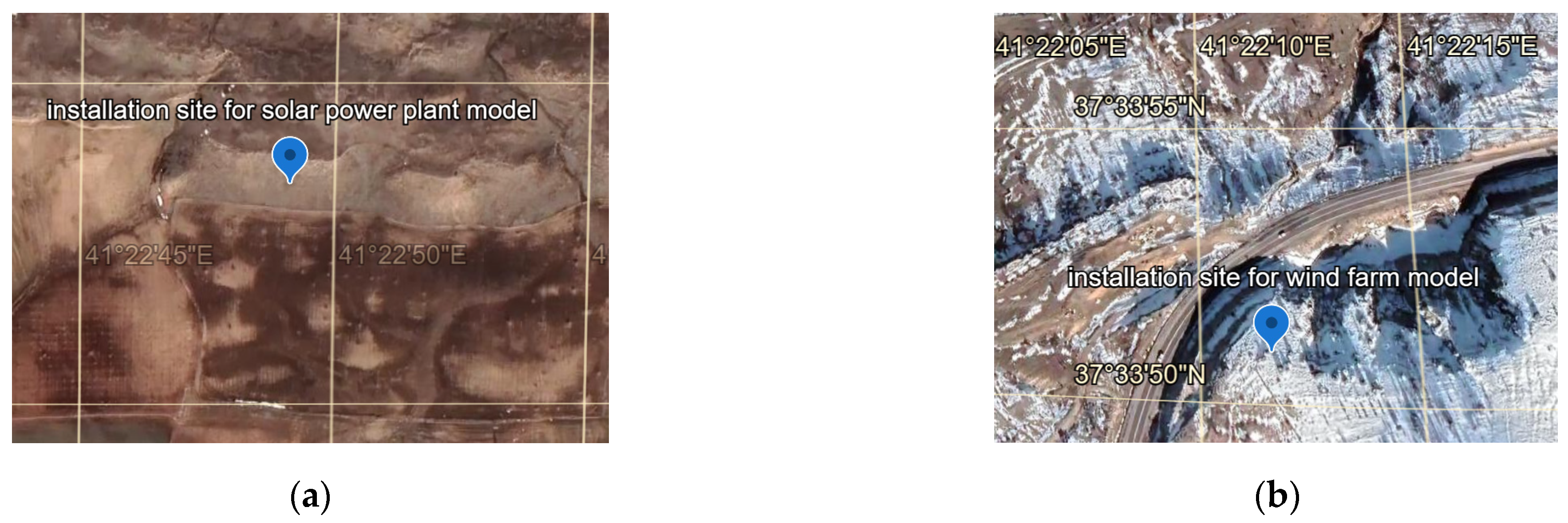
The location information of the installation area for the solar power plant model is 37.3523 N, 41.2249 E, and the location information of the installation area for the wind power plant model is 37.3350 N, 41.2211 E. These locations are shown in Figure 1 [54].

A single dataset with two input parameters was used to estimate the CP. This dataset includes hourly CP values for 2019 and 2020 in the Gercüş district of Batman province in southeast Turkey.

To estimate the GWP, two datasets were used for 2019 and 2020, including active power, wind speed, wind direction, and meteorological parameters that may affect active power production. According to the correlation matrix, parameters that have a very low impact on the prediction result were not used. Two parameters, wind speed (m/s) and wind power (kW), were used as input parameters. The turbine model for the modeled wind power plant was determined to be Vestas V90 2000; the turbine height was 80 m, and the turbine capacity was 1 MW. Meteorological data are taken from MERRA-2 Global (Modern Era Retrospective Analysis for Research and Applications).

In this study, two datasets containing active power, direct radiation, diffuse radiation, and meteorological parameters that may affect active power production for 2019 and 2020 were used to estimate the GSP. According to the correlation matrix, parameters that have a very low impact on the prediction result were not used. Six parameters—irradiance direct (cd/m²), irradiance diffuse (cd/m²), temperature (°C), ground-level solar irradiance (W/m²), and top-of-atmosphere solar irradiance (W/m²)—were used as input parameters. For the modeled solar power plant, the direction the panel faces is 180° (clockwise), the angle of inclination of the panel with the horizontal is 35°, and the total loss rate resulting from the system components is determined to be 0.1. Meteorological data is taken from MERRA-2 Global.

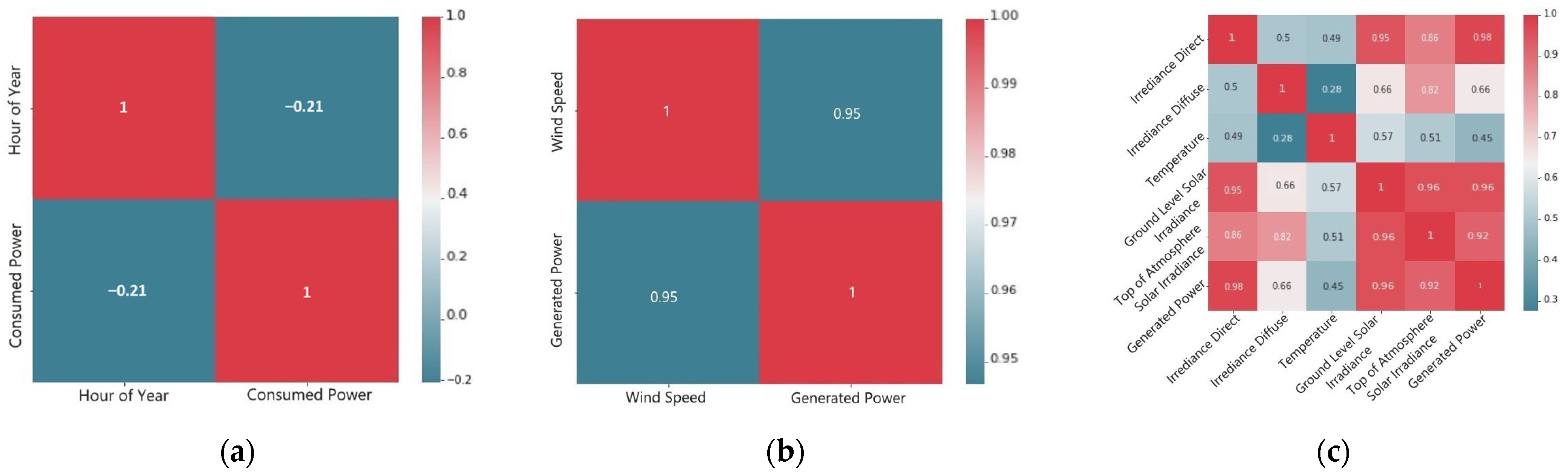
Correlation matrices were used to determine the importance of the effects of the parameters in the dataset regarding the predictions. The relationship between correlation matrices and input and output parameters is expressed with values between −1 and +1. As a result of examining the correlation matrices, input parameters that did not affect the output were removed to increase prediction performance. Figure 2 shows the correlation matrices that express the relationship between the parameters used in the dataset regarding the CP, GWP, and GSP estimates.

Since the input parameters used in estimation methods have different vector values, standardization of these parameters provides significant advantages. In this study, MAPE values were used as the error metric in the PCFE equation. In Equation (5), where the MAPE equation is given, the denominator being zero will make the MAPE value equal to infinity. To overcome this problem and eliminate values of zero, scaling was made between 0.1 and 1. Thus, the MAPE value is prevented from becoming infinite. The normalized value is given by the equation below.

$$X_{scaled}=\{\begin{array}{c}\begin{array}{c}{N}_{min}+\left[\frac{N_{max}-N_{min}}{\left(X_{max}-X_{min}\right)\times 10}\times X_{actual}\right], X_{max}-X_{min}<N_{max}-N_{min}\\ N_{min}+\left(\frac{N_{max}-N_{min}}{X_{max}-X_{min}}\times X_{actual}\right), X_{max}-X_{min}\ge N_{max}-N_{min}\end{array}\end{array}$$

(1)

Here; $X_{scaled}$ is the normalized value; $X_{actual}$ is the original value; $X_{max}$, and $X_{min}$ are the largest and smallest values of the parameter, respectively; and $N_{max}$ and $N_{min}$ are the lowest and highest values of the normalization range, respectively. Since the scaling range is 0.1 to 1, $N_{min}$ = 0.1 and $N_{max}$ = 1.

2.1.2. Network Structures of the Used Forecasting Methods

The datasets used for predictions consist of 17,280 samples. 75% of the dataset was used for training and 25% for testing. The number of epochs for each method was determined as 200. There are no negative values in the datasets used to estimate the wind and solar power produced and the power consumed in the study, and these data are scaled in the range of 0.1–1. The Rectified Linear Unit (ReLU) activation function works faster than other activation functions with its simple structure where it equalizes negative values to 0 and passes positive values as required by $f\left(x\right)=\max \left(0,x\right)$, does not strain the computer hardware, and shortens the training time [55,56,57]. Therefore, ReLU was chosen as the activation function. With its adaptive learning rate and momentum features, Adam Optimizer produces successful results for optimization by using learning rates specific to each parameter and taking into account the gradients in previous stages [39,58]. For this reason, Adam Optimizer was used in machine learning methods used for prediction. The learning rate determines how much the model changes the weights at each step. A high learning rate value allows the model to be trained quickly but reduces convergence. Although a low learning rate value causes the model to be trained slowly, it increases convergence [40]. In order to ensure high convergence in the study, the learning rate value was chosen as 0.0001. As the loss function, the MSE loss function, which is suitable for wind and solar energy production forecasting due to its superior performance in predicting random fluctuations and stationarities in the data, was used [59]. Using these parameters, machine learning methods were used to estimate the CP, GWP, and GSP, and the appropriate method was determined for the most accurate prediction.

Table 2. Network parameters for the MLP algorithm.

Layer	CP		GWP		GSP
	Output Shape	Parameter	Output Shape	Parameter	Output Shape	Parameter
Dense 1	(, 20)	420	(, 20)	420	(, 60)	3660
Dense 2	(, 128)	2688	(, 128)	2688	(, 128)	7808
Dense 3	(, 256)	33,024	(, 256)	33,024	(, 256)	33,024
Dense 4	(, 1)	257	(, 1)	257	(, 1)	257
Total Parameter		36,389		36,389		44,749

,

Table 3. Network parameters for the LSTM algorithm.

Layer	CP		GWP		GSP
	Output Shape	Parameter	Output Shape	Parameter	Output Shape	Parameter
LSTM	(, 200)	162,400	(, 200)	162,400	(, 200)	165,600
Dense 1	(, 128)	25,728	(, 128)	25,728	(, 128)	25,728
Dense 2	(, 256)	33,024	(, 256)	33,024	(, 256)	33,024
Dense 3	(, 1)	257	(, 1)	257	(, 1)	257
Total Parameter		221,409		221,409		224,609

and

Table 4. Network parameters for the CNN algorithm.

Layer	CP		GWP		GSP
	Output Shape	Parameter	Output Shape	Parameter	Output Shape	Parameter
Conv1D 1	(, 9, 64)	320	(, 9, 64)	192	(, 9, 64)	704
Conv1D 2	(, 7, 64)	12,352	(, 7, 64)	12,352	(, 7, 64)	12,352
Conv 1D 3	(, 4, 64)	16,448	(, 4, 64)	16,448	(, 4, 64)	16,448
Max Pooling 1D	(, 2, 64)	0	(, 2, 64)	0	(, 2, 64)	0
Flatten	(, 128)	0	(, 128)	0	(, 128)	0
Dense 1	(, 128)	16,512	(, 128)	16,512	(, 128)	16,512
Dense 2	(, 256)	33,024	(, 256)	33,024	(, 256)	33,024
Dense 3	(, 512)	131,584	(, 512)	131,584	(, 512)	131,584
Dense 4	(, 256)	131,584	(, 256)	131,328	(, 256)	131,328
Dense 5	(, 1)	257	(, 1)	257	(, 1)	257
Total Parameter		341,825		341,697		342,209

show the network structures of MLP, LSTM, and CNN algorithms modeled for prediction, respectively.

2.1.3. Error Metrics

In the study, popular error measurement metrics like R-squared (R²), mean square error (MSE), root mean square error (RMSE), mean absolute error (MAE), and mean absolute percentage error (MAPE) were utilized to assess the prediction accuracy of the MLP, LSTM, and CNN algorithms. When utilizing these parameters to assess the discrepancy between the predicted and actual values, the direction of errors or compensatory effects was ignored. Error measures quantify the extent to which predictions match the real data. R² is a statistical measure whose value ranges from 0 to 1. It is used to assess how many changes in the independent variable can account for change in the dependent variable. MSE represents the mean squared error. RMSE stands for the standard deviation in forecast errors. A lower value of RMSE indicates a superior model. The absolute difference between the variables that were predicted and those that were observed is measured by the MAE. If the units of the error values are different, the MAPE statistics parameter can be used [41].

$$R^2=1-\frac{{{\displaystyle \sum }}_{i=1}^n{\left(x_i-x_i^{*}\right)}^2}{{{\displaystyle \sum }}_{i=1}^n{\left(x_i-\overline{x_i}\right)}^2}$$

(2)

$$RMSE=\sqrt{\frac{1}{n}{\displaystyle \sum }_{i=1}^n{\left(x_i^{*}-x_i\right)}^2}$$

(3)

$$MSE=\frac{1}{n}{\displaystyle \sum }_{i=1}^n{\left(x_i-x_i^{*}\right)}^2$$

(4)

$$MAE=\frac{1}{n}{\displaystyle \sum }_{i=1}^n\left|x_i-x_i^{*}\right|$$

(5)

$$MAPE=\left[\frac{1}{n}{\displaystyle \sum }_{i=1}^n\frac{\left|x_i^{*}-x_i\right|}{x_i}\right]\times 100$$

(6)

In these equations, $x_i$, $x_i^{*}$, and $\overline{x_i}$ represent the actual, predicted, and average actual values respectively, and $n$ also represents the number of samples.

2.2. Expected Power Not Served Formulation and Smart Reserve Planning

This section describes the cost function that minimizes the cost of production, reserves, and EPNS. In the first subsection, the newly developed EPNS formulation resulting from the forecast errors of CP, GWP, and GSP is explained, and in the second subsection, the SRP is explained.

2.2.1. Formulation of Expected Power Not Served

The majority of research in literature computes the CP and GWP estimation errors using the standard deviation-based approach recommended by Ortega-Vazquez et al. [21,30,32,33,34]. According to this method, Equation (7) provides the standard deviation of the CP estimate, and Equation (8) provides the standard deviation of the GWP estimate.

$${\sigma }_l=\frac{k}{100}{l}_A$$

(7)

$${\sigma }_w=\frac{1}{5}{w}_f+\frac{1}{50}{W}_I$$

(8)

In these equations, ${\sigma }_l$ and ${\sigma }_w$ represent the standard deviation of the load forecast and the standard deviation of the GWP forecast, respectively; $k$ represents the accuracy percentage of the load forecasting tool; $l_A$ represents the actual CP value; $w_f$ represents the predicted wind; and $W_I$ represents the total installed wind power. The total standard deviation of the CP and GWP estimation errors is given by Equation (9).

$${\sigma }_d=\sqrt{{\left({\sigma }_l\right)}^2+{\left({\sigma }_w\right)}^2}$$

(9)

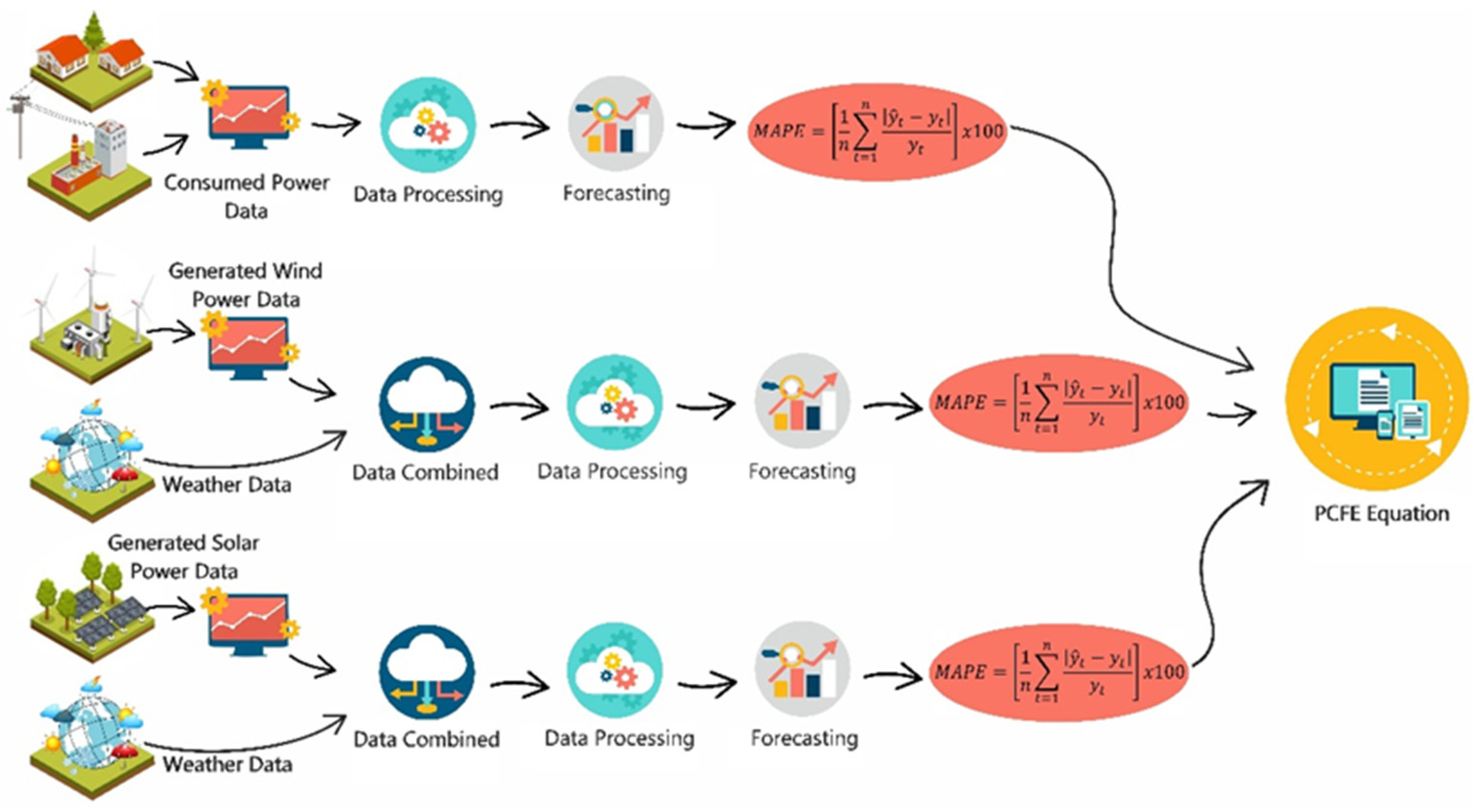
In the above equations, coefficients were needed, and assumptions were made to increase the prediction accuracy. In this study, popular machine learning methods were used to calculate the power capacity of forecast errors (PCFE) resulting from the forecast errors of CP, GWP, and GSP to be used in the EPNS calculation. For this purpose, the MAPE value, which is an error metric, was used to calculate PCFE (kW). Figure 3 shows the flow chart of the PCFE equation.

The PCFE equation obtained using MAPE values for predictions made with MLP, LSTM, and CNN methods is given below.

$$PCFE=P_l^f\times \frac{MAP{E}_l}{100}+P_w^f\times \frac{MAP{E}_w}{100}+P_s^f\times \frac{MAP{E}_s}{100}$$

(10)

where $MAP{E}_l$, $MAP{E}_w$, and $MAP{E}_s$ are the MAPE values for CP estimation, GWP estimation, and GSP estimation, respectively; and $P_l^f$ (kW), $P_w^f$ (kW), and $P_s^f$ (kW) are the forecasts of CP, GWP, and GSP, respectively. In the EPNS formulation resulting from prediction errors, the approach proposed in [21,32,42], where the sum of the produced power and reserve is subtracted from the sum of the CP and the total prediction error capacity, is considered.

$$EPNS=\left[P_l^f+PCFE-\left(P_{total}+R_{total}+P_w^f+P_s^f\right)\right]\times \alpha$$

(11)

where EPNS (kW) is the unprovided power resulting from forecast errors; $P_{total}$ (kW) is the total power output of the conventional generation units; and $R_{total}$ (kW) is the total reserve available from conventional generation units. The $P_{total}$ value for reserve adjustment is calculated by Equation (12). Moreover, $\alpha$ indicates whether there are consumers to whom power cannot be transferred. This value equals 1 when the system demand is greater than the total available power allocated plus the number of reserves provided, and 0 when the system demand is less than or equal to the total available power plus the number of reserves provided. The state of the $\alpha$ variable is expressed by Equation (13).

$$P_{total}=\{\begin{array}{c}0;P_l^f\le P_w^f+P_s^f\\ \left[P_l^f-\left(P_w^f+P_s^f\right)\right]; P_l^f>P_w^f+P_s^f\end{array}$$

(12)

$$\alpha =\{\begin{array}{c}1;P_{total}+R_{total}+P_w^f+P_s^f<P_l^f+PCFE\\ 0; P_{total}+R_{total}+P_w^f+P_s^f\ge P_l^f+PCFE\end{array}$$

(13)

In this study, unit allocation planning was adopted, taking into account the reserve requirement for one hour later. The reserve requirement for each hour is calculated according to the $EPN{S}_{max}$ value, which is the reliability criterion determined by the system operator. This calculation is performed using the EPNS evaluation criterion given in Equation (14).

$$EPNS\le EPN{S}_{max}$$

(14)

2.2.2. Smart Reserve Planning and Cost Function

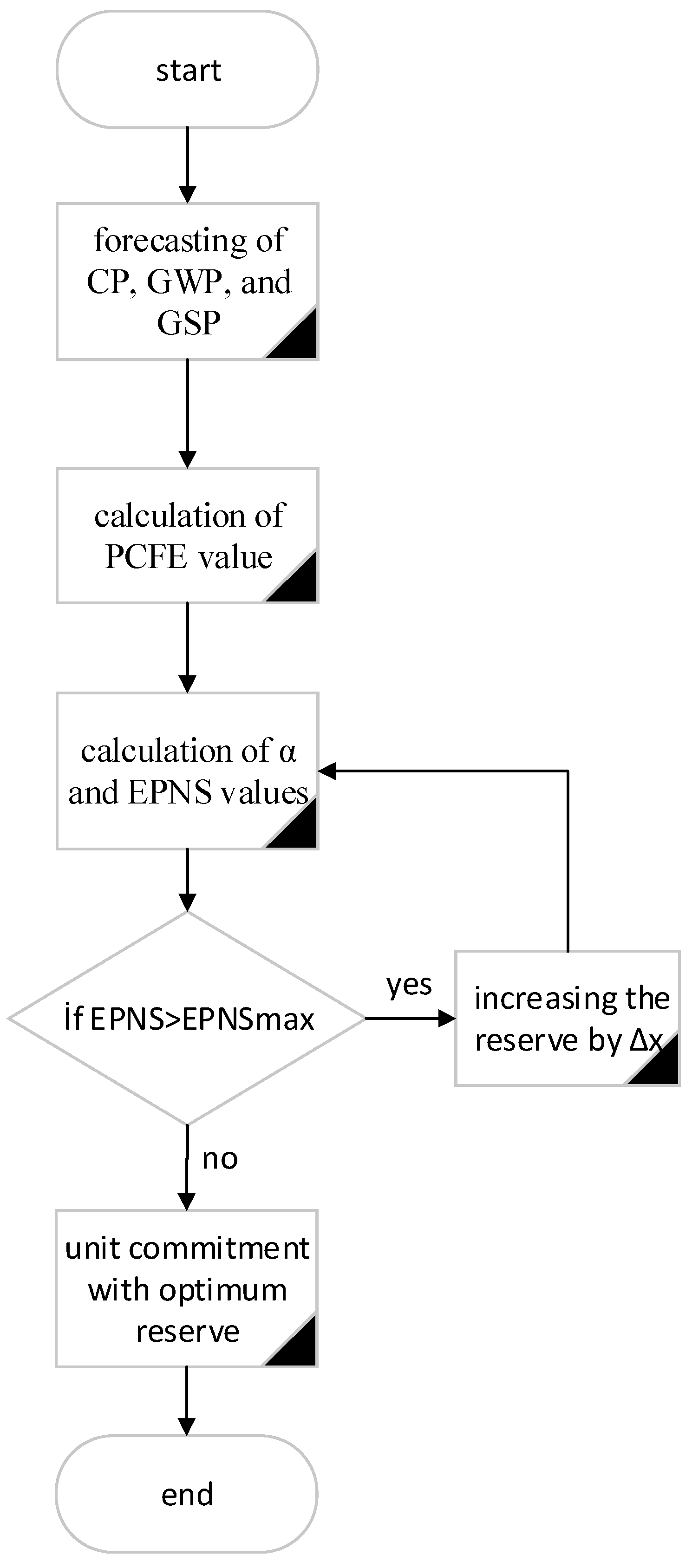
For reliability and flexibility in power systems based on renewable energy, reserve planning is made with the limit EPNS value determined by the power system operator. The SRP process diagram is displayed in Figure 4. The SRP process is summarized as follows:

• Making CP, GWP, and GSP predictions using the CNN algorithm, which gives the best results among the prediction algorithms.
• Calculation of PCFE value using CP, GWP, and GSP estimates.
• Calculating the α variable and then calculating the EPNS value in the power system.
• Comparison of the calculated EPNS value with the limit EPNS value determined by the power system operator.
• If EPNS > EPNS_max, the reserve is increased by ∆x, and the process continues by recalculating the EPNS value and the α variable. This cycle continues until the EPNS ≤ EPNS_max condition is met. In the study, the ∆x value for the sample power system was determined as 0.1 kW.
• When the EPNS ≤ EPNS_max condition is met, the unit commitment is made, and the process ends.

The cost function for the unit commitment minimizes the cost as a result of power planning and SRP produced by taking into account the cost/benefit analysis proposed by Ortega-Vazquez and Kirschen [36] is given by Equation (15).

$$TC=min\left(P_{total}\times C_o+R_{total}\times C_r+EPNS\times VOLL\right)$$

(15)

Here, TC represents the system total cost; $C_o$ represents the operating cost of traditional production units; $C_r$ represents the reserve provision cost of traditional production units; and VOLL represents the value of lost load. The VOLL value is calculated as a result of statistical research. This value may have a different value for each system in response to the energy that cannot be provided.

3. Analysis and Results

In Section 3.1, results regarding the accuracy of the prediction methods are given. In Section 3.2, results regarding SRP and cost are given using the newly developed EPNS formula.

3.1. Studies on Forecasting Methods

This section contains the application results of the methods used in Section 2.1 to estimate the CP and the power produced from intermittent sources. In Section 3.1.1, results regarding the network training processes of the prediction methods used are given. In Section 3.1.2, results regarding the accuracy of the estimation methods used are given. The algorithms were modeled and implemented with a Monster Notebook running Python 3.11 [60]. The hardware of the machine features an Intel™ Core™ i7-9750H CPU at 2.60 GHz, 16 GB of 2667 MHz RAM, and an NVIDIA GeForce RTX 2070 8 GB GPU. Prediction algorithms were created using the TensorFlow 2.3.0 software library. This library makes the code more interactive and comprehensible while also offering improved performance and simplicity of usage.

3.1.1. Network Training Processes Regarding the Prediction Methods

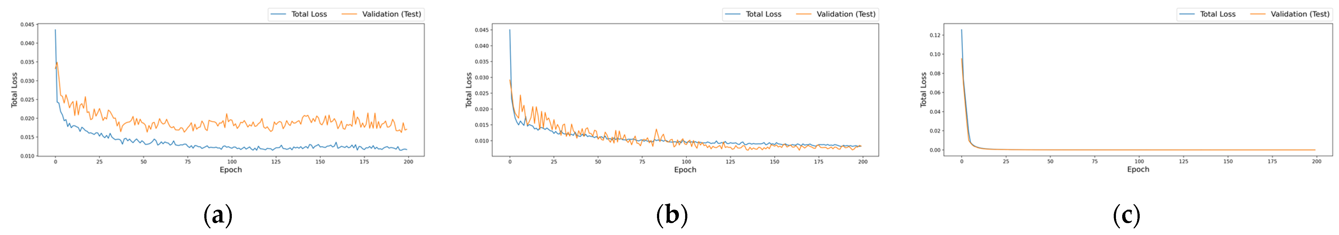
Figure 5, Figure 6 and Figure 7 show the graphs for the network training process of the methods used to estimate the CP, GWP, and GSP, respectively. In these graphs, loss is a metric that expresses how far the actual values deviate from the predictions of a model. A graph that illustrates how a model’s loss varies as it is trained is called a loss curve. Because the model learns from the data, the loss should typically decrease as the training process goes on. Since the model has not had experience learning how to adjust to the data, the loss curve is typically high when training first starts. As the model improves, the loss value typically drops after the first epoch, or iterations. Typically, the loss curve finds its optimal position, and as a result, this position is where the model performs best. In this study, models were trained for 200 epochs. When the graphs are examined, it is seen that the loss value decreases for all three algorithms used. Among the algorithms, the most successful model for predicting CP, GWP, and GSP appears to be the CNN algorithm, which reaches zero loss almost before 25 epochs.

3.1.2. Accuracy of Prediction Methods

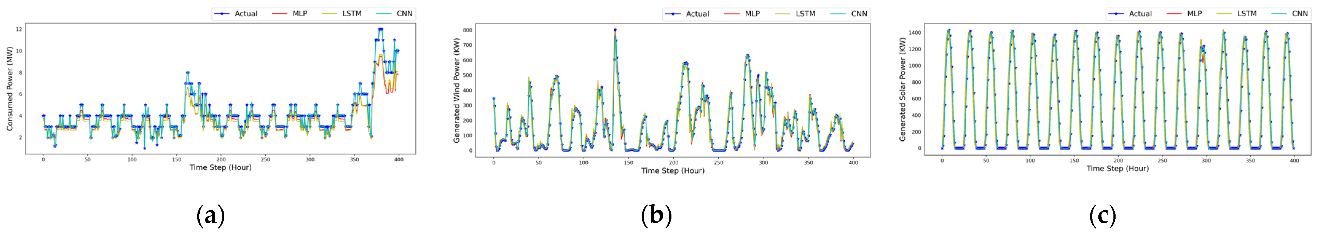
Figure 8 shows the accuracy of the CP, GWP, and GSP estimation algorithms developed with MLP, LSTM, and CNN methods, respectively. For this purpose, the prediction results for 400 samples of the test data were compared with the actual values. When the graphs are examined, it is seen that the CNN algorithm is more successful than other algorithms.

Table 5. Error metrics parameter values for the algorithms used for prediction.

Error Metrics	CP			GWP			GSP
	MLP	LSTM	CNN	MLP	LSTM	CNN	MLP	LSTM	CNN
R2	0.65218	0.73558	0.99473	0.96038	0.96136	0.99904	0.97938	0.99586	0.99959
MSE	0.00236	0.00179	4 × 10−5	0.00099	0.00097	2 × 10−5	0.00152	0.00031	3 × 10−5
RMSE	0.04855	0.04233	0.00598	0.03147	0.03108	0.00491	0.03898	0.01748	0.00551
MAE	0.03707	0.03275	0.00424	0.01712	0.01689	0.00248	0.01929	0.00784	0.0032
MAPE	11.3498	10.6392	1.4961	6.749	6.9987	1.0776	7.4123	2.951	1.4512

shows the R², MSE, RMSE, MAE, and MAPE error metrics parameter values for the algorithms used for prediction. When the table is examined, it can be seen that the method with the lowest prediction error is the CNN algorithm.

3.2. Studies on Smart Reserve Planning and Total Cost

The work carried out in Section 3.2.1 shows how the accuracy of forecasts affects the reserve requirement and the overall cost. The study in Section 3.2.2 examined the impact of intermittent source penetration on the reserve requirement and overall cost. In Section 3.2.3, a sensitivity study is conducted to show how power system reliability affects reserve requirements and overall costs. The study is carried out on modeled wind and solar power plants in the Gercüş district of Batman province. Normal operating costs of thermal generation units are determined at 3 cents per kWh, and reserve provision costs are determined at 15 cents per kWh. VOLL was determined as 4 USD/kWh. For SRP, the ∆x value in Figure 3 is determined to be 0.1 kW. Since this value was chosen as small, reserve planning was made for a value equal to or very close to the $EPN{S}_{max}$ value allowed by the system operator. The reserve requirement is determined by the EPNS value calculated according to the evaluation criteria given in Equation (10). Cost/benefit analysis was used to determine the optimum total cost according to this criterion, which determines system reliability. The lowest total cost is achieved when the system operates under optimum conditions. System operators can purchase the appropriate number of reserves at the most economical price by using cost/benefit analysis. Application results are shown for the first 150 h of test data.

3.2.1. The Impact of Forecast Accuracy on Reserve Requirement and Total Cost

In this subsection, the results obtained with the predictions made by MLP, LSTM, and CNN methods are compared to examine the effect of prediction accuracy on reserve requirements and total costs. Reserve requirement curves for predictions made with MLP, LSTM, and CNN methods are shown in Figure 9. When Figure 9 is examined, the lowest reserve requirement for the 5 kW $EPN{S}_{max}$ value was obtained by estimation using the CNN method. This result shows that accuracy in forecasts reduces the reserve requirement.

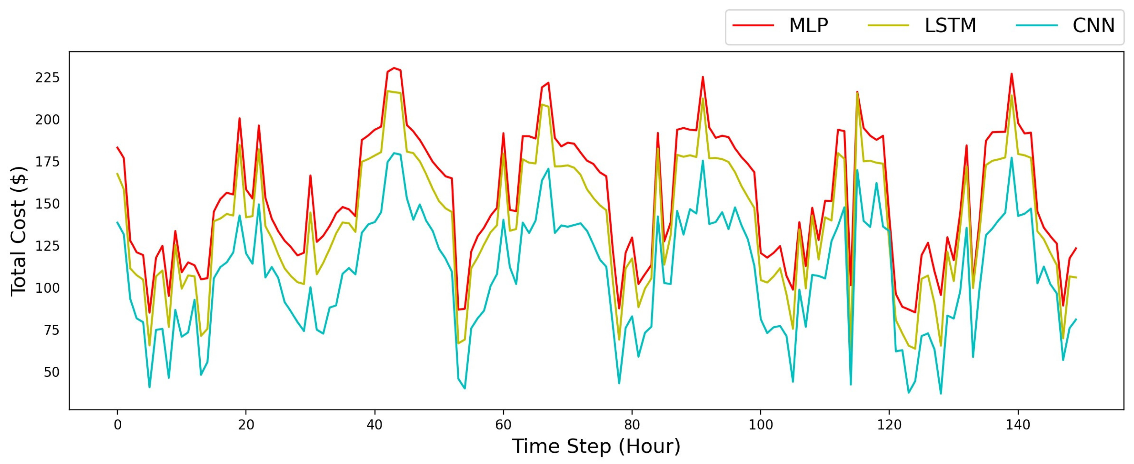
Figure 10 shows the total cost of the power system as a result of the predictions made with MLP, LSTM, and CNN methods. Figure 10 shows that the lowest total cost was obtained with the estimation made with the CNN method. This result shows that accuracy in predictions reduces the total cost.

3.2.2. Effect of Intermittent Source Penetration on Reserve Requirement and Total Cost

In this section, four different cases are considered to evaluate the sensitivity of the reserve requirement and total cost to the level of intermittent resource penetration. These cases are as follows:

Case 1: Presence of solar and wind power plants along with traditional production units in the power system.

Case 2: Presence of only wind power plants along with traditional generation units in the power system.

Case 3: Presence of only solar power plants along with traditional generation units in the power system.

Case 4: Presence of only conventional generation plants in the power system.

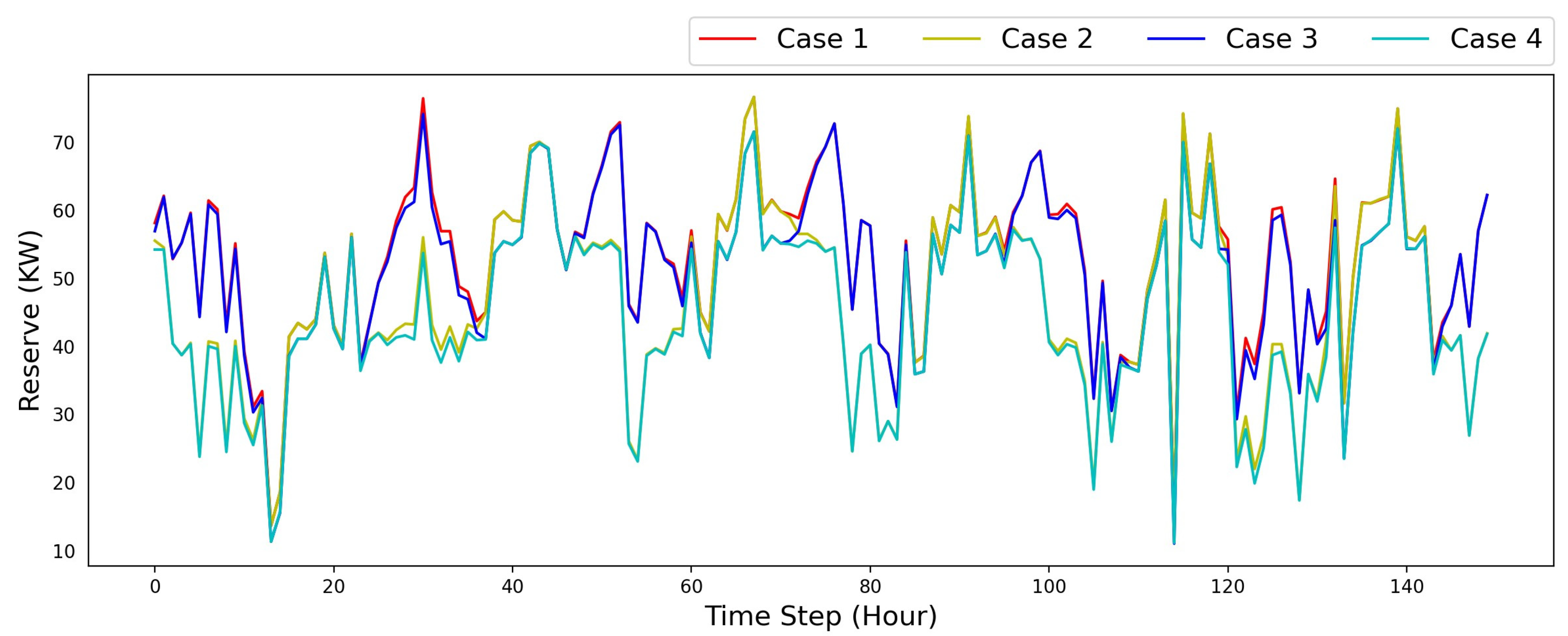
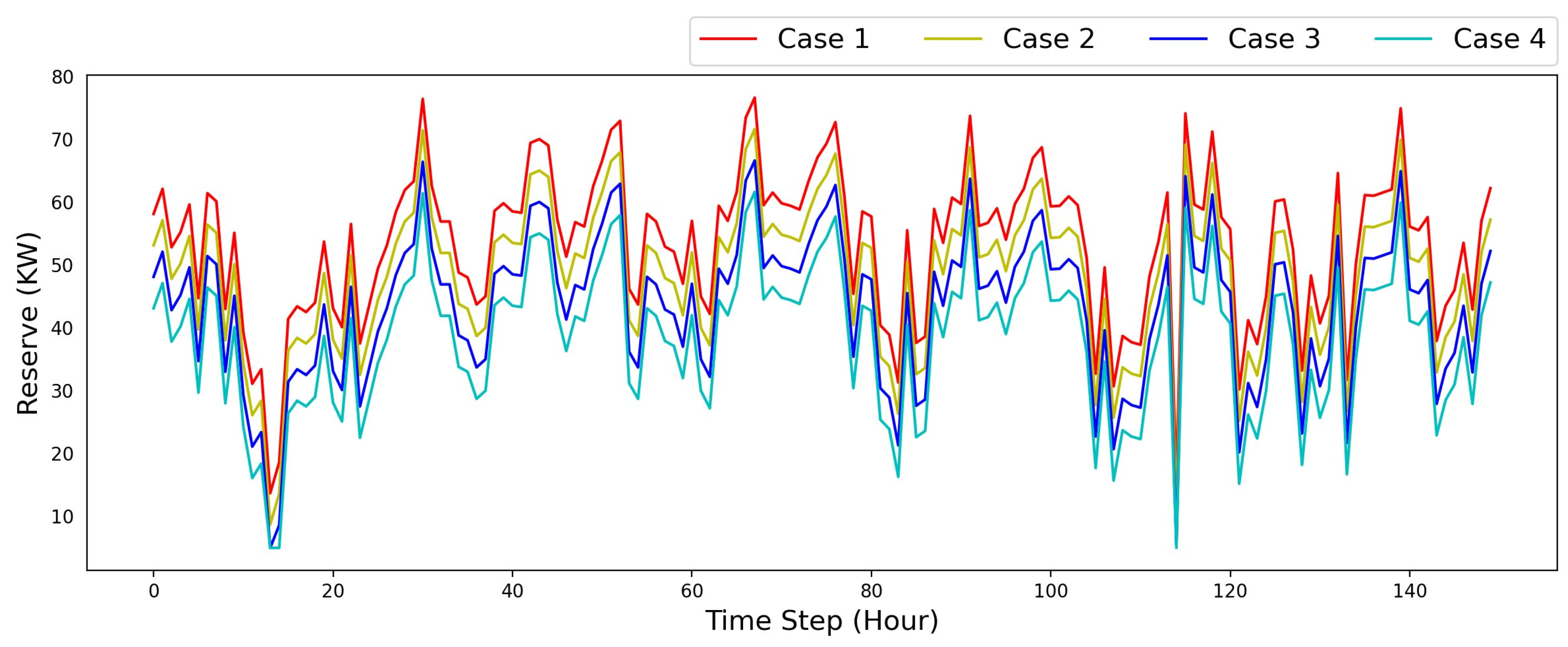
Figure 11 shows the reserve requirement according to different IRES penetration cases using the CNN algorithm, which provides the most accurate prediction result. In Figure 11, it can be seen that the highest reserve requirement for the 5 kW $EPN{S}_{max}$ value is caused when there are wind and solar power plants in the system, that is, at the highest intermittent source penetration level. It is seen that when there is a solar power plant with an installed capacity of 2 MW in the system, the reserve requirement is higher than when there is a 1 MW wind power plant. Important parameters such as the average wind speed and irradiance levels in the regions where they are located, along with the installed power of the power plants, explain this situation. It is seen that the reserve requirement is at its lowest level when there are no intermittent resources in the system. As a result, it can be concluded that the reserve requirement increases with the increase in the penetration level of intermittent generation sources in power systems.

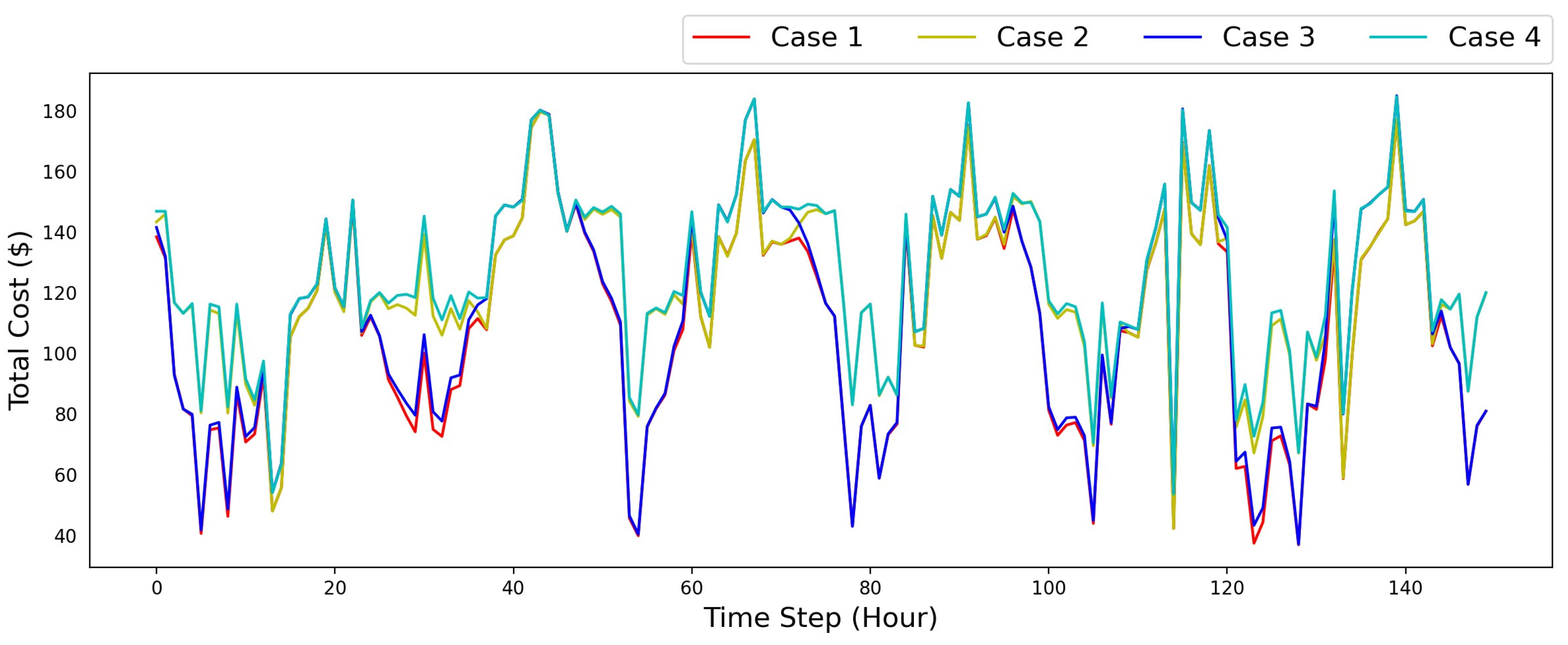
Figure 12 shows the total cost according to different IRES penetration cases using the CNN algorithm, which provides the most accurate prediction result. Figure 12 shows that the lowest total cost for a 5 kW $EPN{S}_{max}$ value is achieved when wind and solar power plants are present in the system or when the system is at the highest intermittent source penetration level. It can be seen in the figure that the total cost of the system containing a solar power plant with 2 MW of installed power is less than the total cost of the system containing a wind power plant with 1 MW of installed power. This situation can be explained by basic factors such as the installed power of the power plants, the average wind speed, and the radiation levels in their locations. In addition, it is seen that the total cost is at its maximum level when there are no intermittent resources in the system. Therefore, it may be concluded that as intermittent generation becomes more prevalent in power systems, costs will decrease.

3.2.3. Effect of System Reliability on Reserve Requirement and Total Cost

In Equation (10), where the reliability evaluation criterion for the power system is given, increasing the $EPN{S}_{max}$ value will cause an increase in the power that cannot be transferred to the consumer. This will reduce the reliability of the power system. In this section, the effect of system reliability on the reserve requirement and total cost is evaluated by considering four cases in which different $EPN{S}_{max}$ values are used. $EPN{S}_{max}$ value is determined as 5 kW in Case 1, 10 kW in Case 2, 15 kW in Case 3, and 20 kW in Case 4.

Figure 13 shows the reserve requirements for different $EPN{S}_{max}$ values using the CNN algorithm, which provides the most accurate prediction result. Figure 13 shows that the reserve requirement is at its highest level when the $EPN{S}_{max}$ value is 5 kW. It is seen that the reserve amount decreases when the $EPN{S}_{max}$ value increases. This situation causes a decrease in system reliability.

Figure 14 shows the total costs for different EPNS_max values using the CNN algorithm, which provides the most accurate prediction result. Accordingly, it is understood that the total cost is at its lowest when the EPNS_max value is 5 kW, and when this value increases, the total cost also increases. Increasing EPNS_max reduces the reserve requirement. As the reserve amount decreases, the cost of providing reserves decreases, but the amount of power that cannot be provided to consumers also increases. Increasing EPNS_max also reduces the reliability of the power system. Decreasing power system reliability will lead to an increase in the number of consumers to whom the power system cannot transmit power, which will create additional penalty costs. As a result, it has been concluded that increasing the reliability of the power system will also increase the cost.

4. Conclusions

In this study, CP, GWP, and GSP forecast errors were included in the EPNS calculation process with a new method. The EPNS formulation was created with the PCFE value obtained from predictions made with machine learning methods. In the proposed method, the MAPE value, which is one of the error parameters measuring the prediction accuracy, was used in the PCFE calculation.

The R² values obtained from MLP, LSTM, and CNN methods for GWP estimation are 0.96038, 0.96136, and 0.99904, respectively. Despite the superior performance of all methods, the best result was obtained with the CNN method. The R² values obtained by MLP, LSTM, and CNN methods for GSP estimation are 0.97938, 0.99586, and 0.99959, respectively. Although all methods showed successful performance for GSP estimation, the best result was obtained with the CNN method. Because the study examined a power system feeding a relatively small area, CP data is inconsistent. The R² values for MLP, LSTM, and CNN methods for CP estimation are 0.65218, 0.73558, and 0.99038, respectively. As a result, although the performance of MLP and LSTM methods is low, the CNN method showed superior performance with an R² value of 0.99473. Due to these results, SRP, reliability, and total cost analyses were performed with the CNN method.

The effects of forecast accuracy on reserve requirement and total cost were examined. Accordingly, according to the results obtained with the CNN method, which gives the most successful prediction results, the planned reserve amount at the 20th hour was ~52 kW and the total cost was USD ~121. Additionally, the effect of IRES penetration in the power system on the reserve requirement and total cost was examined. Looking at the 20th hour values, the highest reserve requirement occurred in the case of the highest IRES penetration with ~42 kW, while the highest cost occurred in the case of no IRES in the power system with USD ~135. Finally, the effects of power system reliability on reserve requirement and total cost were examined. When the 20th hour values are examined, the planned reserve amount is at the highest value with ~44 kW when the power system reliability is at its highest, that is, when EPNS_max is 5 kW. The highest total cost, with USD ~182, occurred when the power system reliability was lowest, that is, EPNS_max was 20 kW.

In this article, as a result of forecasts made with different methods, it is shown that the increase in forecast errors increases the reserve requirement and total cost. It has been demonstrated that the increase in the intermittent source penetration level in the power system, although it reduces the total cost, increases the reserve requirement and negatively affects the system reliability. It was concluded that increasing the EPNS_max value determined by the power system operator reduces the reserve requirement but increases the total cost as a result of the increase in unprovided power and the increase in expected outage costs.

Since advanced prediction algorithms are used in the new EPNS formulation, the power that cannot be provided will be reduced. This will reduce the reserve requirement and total cost. Regarding system economy and reliability, this study provides a useful proposal for the integration of intermittent renewable energy sources, such as solar and wind power plants, into power systems.

In future studies, reserve planning approaches including energy storage systems will provide significant advantages in the integration of wind and solar-based production plants. In addition, costs can be reduced by including demand-side management approaches in the reserve planning process.

References

- Bahramara, S.; Moghaddam, M.P.; Haghifam, M.R. Optimal planning of hybrid renewable energy systems using HOMER: A review. Renew. Sust. EnergyRev. 2016, 62, 609–620. [Google Scholar] [CrossRef]
- Neto, P.B.L.; Saavedra, O.R.; Oliveira, D.Q. The effect of complementarity between solar, wind and tidal energy in isolated hybrid microgrids. Renew. Energy 2020, 147, 339–355. [Google Scholar] [CrossRef]
- Alam, M.S.; Al-Ismail, F.S.; Salem, A.; Abido, M.A. High-Level Penetration of Renewable Energy Sources Into Grid Utility: Challenges and Solutions. IEEE Access 2020, 8, 190277–190299. [Google Scholar] [CrossRef]
- Jurasz, J.; Dąbek, P.; Kaźmierczak, B.; Kies, A.; Wdowikowski, M. Large scale complementary solar and wind energy sources coupled with pumped-storage hydroelectricity for Lower Silesia (Poland). Energy 2018, 161, 183–192. [Google Scholar] [CrossRef]
- Ssekulima, E.B.; Anwar, M.B.; Hinai, A.A.; Moursi, M.S.E. Wind speed and solar irradiance forecasting techniques for enhanced renewable energy integration with the grid: A review. IET Renew. Power Gener. 2016, 10, 885–989. [Google Scholar] [CrossRef]
- Liang, X. Emerging power quality challenges due to ıntegration of renewable energy sources. IEEE Trans. Ind. Appl. 2017, 53, 855–866. [Google Scholar] [CrossRef]
- Paoli, C.; Voyant, C.; Muselli, M.; Nivet, M. Forecasting of preprocessed daily solar radiation time series using neural networks. Sol. Energy 2010, 84, 2146–2160. [Google Scholar] [CrossRef]
- Zhang, J.; Yan, J.; Infield, D.; Liu, Y.; Lien, F. Short-term forecasting and uncertainty analysis of wind turbine power based on long short-term memory network and Gaussian mixture model. Appl. Energy 2019, 241, 229–244. [Google Scholar] [CrossRef]
- Shobanadevi, A.; Maragatham, D.; Prabu, M.; Boopathi, K. Short-Term Wind Power Forecasting Using R-LSTM. Int. J. Renew. Energy Res. 2021, 11, 392–406. [Google Scholar] [CrossRef]
- Solas, M.; Cepeda, N.; Viegas, J. Convolutional Neural Network for Short-term Wind Power Forecasting. In Proceedings of the 2019 IEEE PES Innovative Smart Grid Technologies Europe (ISGT-Europe), Bucharest, Romania, 29 September–2 October 2019; pp. 1–5. [Google Scholar] [CrossRef]
- Olanrewaju, O.; Mbohwa, C. Comparison of artificial intelligence techniques for energy consumption estimation. In Proceedings of the 2016 IEEE Electrical Power and Energy Conference (EPEC), Ottawa, ON, Canada, 12–14 October 2016; pp. 1–5. [Google Scholar] [CrossRef]
- Dragomir, O.; Dragomir, F.; Brezeanu, I.; Minca, E. MLP neural network as load forecasting tool on short- term horizon. In Proceedings of the 2011 19th Mediterranean Conference on Control & Automation (MED), Corfu, Greece, 20–23 June 2011; pp. 1265–1270. [Google Scholar] [CrossRef]
- Wang, H.; Li, H.; Gao, S.; Zhou, L.; Lao, Z. Multigranularity Building Energy Consumption Prediction Method Based on Convolutional Recurrent Neural Network. Wirel. Commun. Mob. Comput. 2022, 2022, 8524034. [Google Scholar] [CrossRef]
- Elsaraiti, M.; Merabet, A. A comparative analysis of the arıma and lstm predictive models and their effectiveness for predicting wind speed. Energies 2021, 14, 6782. [Google Scholar] [CrossRef]
- Tawn, R.; Browell, J. A review of very short-term wind and solar power forecasting. Renew. Sust. Energy Rev. 2022, 153, 111758. [Google Scholar] [CrossRef]
- Ahmed, R.; Sreeram, V.; Mishra, Y.; Arif, M.D. A review and evaluation of the state-of-the-art in PV solar power forecasting: Techniques and optimization. Renew. Sust. Energy Rev. 2020, 124, 109792. [Google Scholar] [CrossRef]
- Mason, K.; Duggan, J.; Howley, E. Forecasting energy demand, wind generation and carbon dioxide emissions in Ireland using evolutionary neural networks. Energy 2018, 155, 705–720. [Google Scholar] [CrossRef]
- Rahman, M.; Shakeri, M.; Tiong, S.; Khatun, F.; Amin, N.; Pasupuleti, J.; Hasan, M. Prospective methodologies in hybrid renewable energy systems for energy prediction using artificial neural networks. Sustainability 2021, 13, 2393. [Google Scholar] [CrossRef]
- Matos, M.A.; Bessa, R.J. Setting the operating reserve using probabilistic wind power forecasts. IEEE Trans. Power Syst. 2010, 26, 594–603. [Google Scholar] [CrossRef]
- Aazami, R.; Iranmehr, H.; Tavoosi, J.; Mohammadzadeh, A.; Sabzalian, M.H.; Javadi, M.S. Modeling of transmission capacity in reserve market considering the penetration of renewable resources. Int. J. Electr. Power Energy Syst. 2023, 145, 108708. [Google Scholar] [CrossRef]
- Zhang, M.; Jiao, Z.; Ran, L.; Zhang, Y. Optimal energy and reserve scheduling in a renewable-dominant power system. Omega 2023, 118, 102848. [Google Scholar] [CrossRef]
- Xu, Y.; Wan, C.; Liu, H.; Zhao, C.; Song, Y. Probabilistic forecasting-based reserve determination considering multi-temporal uncertainty of renewable energy generation. IEEE Trans. Power Syst. 2023, 39, 1019–1031. [Google Scholar] [CrossRef]
- Auguadra, M.; Ribó-Pérez, D.; Gómez-Navarro, T. Planning the deployment of energy storage systems to integrate high shares of renewables: The Spain case study. Energy 2023, 264, 126275. [Google Scholar] [CrossRef]
- Khatami, R.; Parvania, M.; Narayan, A. Flexibility reserve in power systems: Definition and stochastic multi-fidelity optimization. IEEE Trans. Smart Grid 2019, 11, 644–654. [Google Scholar] [CrossRef]
- Fernández-Muñoz, D.; Pérez-Díaz, I.J. Optimisation models for the day-ahead energy and reserve self-scheduling of a hybrid wind–battery virtual power plant. J. Energy Storage 2023, 57, 106296. [Google Scholar] [CrossRef]
- Deng, X.; Lv, T. Power system planning with increasing variable renewable energy: A review of optimization models. J. Clean. Prod. 2020, 246, 118962. [Google Scholar] [CrossRef]
- Roald, L.A.; Pozo, D.; Papavasiliou, A.; Molzahn, D.K.; Kazempour, J.; Conejo, A. Power systems optimization under uncertainty: A review of methods and applications. Electr. Power Syst. Res. 2023, 214, 108725. [Google Scholar] [CrossRef]
- Bouffard, F.; Galiana, F.D.; Conejo, A.J. Market-clearing with stochastic security-part I: Formulation. Electr. Power Syst. Res. 2005, 20, 1818–1826. [Google Scholar] [CrossRef]
- Al-Shaalan, M.A. Reliability evaluation in generation expansion planning based on the expected energy not served. J. King Saud. Univ. Eng. Sci. 2012, 24, 11–18. [Google Scholar] [CrossRef]
- Toh, G.K.; Gooi, H.B. Incorporating forecast uncertainties into EENS for wind turbine studies. Electr. Power Syst. Res. 2011, 81, 430–439. [Google Scholar] [CrossRef]
- Liu, G.; Tomsovic, K. Quantifying Spinning Reserve in Systems With Significant Wind Power Penetration. IEEE Trans. Power Syst. 2012, 27, 2385–2393. [Google Scholar] [CrossRef]
- Ortega-Vazquez, M.A.; Kirschen, S.D. Estimating the spinning reserve requirements in systems with significant wind power generation penetration. IEEE Trans. Power Syst. 2009, 24, 114–124. [Google Scholar] [CrossRef]
- Bouffard, F.; Galiana, F.D. Stochastic security for operations planning with significant wind power generation. In Proceedings of the 2008 IEEE Power and Energy Society General Meeting-Conversion and Delivery of Electrical Energy in the 21st Century, Pittsburgh, PA, USA, 20–24 July 2008; pp. 1–11. [Google Scholar] [CrossRef]
- Chaiyabut, N.; Damrongkulkumjorn, P. Optimal spinning reserve for wind power uncertainty by unit commitment with EENS constraint. In Proceedings of the ISGT 2014, Washington, DC, USA, 19–22 February 2014; pp. 1–5. [Google Scholar] [CrossRef]
- Chen, Q.; Folly, K. Effect of ınput features on the performance of the ann-based wind power forecasting. In Proceedings of the 2019 Southern African Universities Power Engineering Conference/Robotics and Mechatronics/Pattern Recognition Association of South Africa (SAUPEC/RobMech/PRASA), Bloemfontein, South Africa, 28–30 January 2019; pp. 673–678. [Google Scholar] [CrossRef]
- Wu, Q.; Guan, F.; Lv, C.; Huang, Y. Ultra-short-term multi-step wind power forecasting based on CNN-LSTM. IET Renew. Power Gener. 2021, 15, 1019–1029. [Google Scholar] [CrossRef]
- Abumohsen, M.; Owda, A.Y.; Owda, M. Electrical load forecasting using LSTM, GRU, and RNN algorithms. Energies 2023, 16, 2283. [Google Scholar] [CrossRef]
- Lim, S.; Huh, J.; Hong, S.; Park, C.; Kim, J. Solar Power Forecasting Using CNN-LSTM Hybrid Model. Energies 2022, 15, 8233. [Google Scholar] [CrossRef]
- Kariniotakis, G.; Stavrakakis, G.; Nogaret, E. Wind power forecasting using advanced neural networks models. IEEE Trans. Energy Convers. 1996, 11, 762–767. [Google Scholar] [CrossRef]
- Wang, H.; Xue, W.; Liu, Y.; Peng, J.; Jiang, H. Probabilistic wind power forecasting based on spiking neural network. Energy 2020, 196, 117072. [Google Scholar] [CrossRef]
- Karaman, Ö.A. Prediction of wind power with machine learning models. Appl. Sci. 2023, 13, 11455. [Google Scholar] [CrossRef]
- Ortega-Vazquez, M.A.; Kirschen, D.S. Optimizing the spinning reserve requirements using a cost/benefit analysis. IEEE Trans. Power Syst. 2007, 22, 24–33. [Google Scholar] [CrossRef]
- Onyari, E.K.; Ikotun, B.D. Prediction of compressive and flexural strengths of a modified zeolite additive mortar using artificial neural network. Constr. Build. Mater. 2018, 187, 1232–1241. [Google Scholar] [CrossRef]
- Almeida, J. Predictive non-linear modeling of complex data by artificial neural networks. Curr. Opin. Biotechnol. 2002, 13, 72–76. [Google Scholar] [CrossRef]
- Hanifi, S.; Liu, X.; Lin, X.; Lotfian, Z. A critical review of wind power forecasting methods—Past, present and future. Energies 2020, 13, 3764. [Google Scholar] [CrossRef]
- Park, Y.S.; Lek, S. Artificial neural networks: Multilayer perceptron for ecological modelin. Dev. Environ. Model. 2016, 28, 123–140. [Google Scholar] [CrossRef]
- Filippi, A.M.; Jensen, J.R. Fuzzy learning vector quantization for hyperspectral coastal vegetation classification. Remote Sens. Environ. 2006, 100, 512–530. [Google Scholar] [CrossRef]
- Lechner, M.; Hasani, R. Learning long-term dependencies in ırregularly-sampled time series. arXiv 2020, arXiv:2006.04418. [Google Scholar] [CrossRef]
- Lindemann, B.; Maschler, B.; Sahlab, N.; Weyrich, M. A survey on anomaly detection for technical systems using LSTM networks. Comput. Ind. 2021, 131, 103498. [Google Scholar] [CrossRef]
- Erkan, E.; Arserim, M.A. Mobile robot application with hierarchical start position dqn. Comput. Intell. Neurosci. 2022, 2022, 4115767. [Google Scholar] [CrossRef]
- Moreno, S.R.; Seman, L.O.; Stefenon, S.F.; dos Santos Coelho, L.; Mariani, V.C. Enhancing wind speed forecasting through synergy of machine learning, singular spectral analysis, and variational mode decomposition. Energy 2024, 292, 130493. [Google Scholar] [CrossRef]
- [dataset] Turkey Electric Transmission Inc. (TEİAŞ), Hourly Consumed Power Data for the Gercüş District of Batman Province in Southeastern Turkey for the Years 2019 and 2020; Turkey Electric Transmission Inc.: Batman, Turkey, 2019. [Google Scholar]
- Renewables Ninja. Available online: https://www.renewables.ninja/ (accessed on 5 November 2023).
- Google Earth. Available online: https://earth.google.com/web/ (accessed on 3 November 2023).
- Ko, M.; Lee, K.; Kim, J.; Hong, C.; Dong, Z.; Hur, K. Deep Concatenated Residual Network With Bidirectional LSTM for One-Hour-Ahead Wind Power Forecasting. IEEE Trans. Sustain. Energy 2020, 12, 1321–1335. [Google Scholar] [CrossRef]
- Koh, N.; Sharma, A.; Xiao, J.; Peng, X.; Woo, W. Solar Irradiance Forecast using Long Short-Term Memory: A Comparative Analysis of Different Activation Functions. In Proceedings of the 2022 IEEE Symposium Series on Computational Intelligence (SSCI), Singapore, 4–7 December 2022; pp. 1096–1101. [Google Scholar] [CrossRef]
- Ling, Z.; Zhou, B.; Or, S.; Cao, Y.; Wang, H.; Li, Y.; Chan, K. Spatio-temporal wind speed prediction of multiple wind farms using capsule network. Renew. Energy 2021, 175, 718–730. [Google Scholar] [CrossRef]
- Tian, Y.; Wang, D.; Zhou, G.; Wang, J.; Zhao, S.; Ni, Y. An Adaptive Hybrid Model for Wind Power Prediction Based on the IVMD-FE-Ad-Informer. Entropy 2023, 25, 647. [Google Scholar] [CrossRef]
- Islam, M.; Nagrial, M.; Rizk, J.; Hellany, A. Solar Radiation and Wind Speed Forecasting using Deep Learning Technique. In Proceedings of the 2021 IEEE Asia-Pacific Conference on Computer Science and Data Engineering (CSDE), Brisbane, Australia, 8–10 December 2021; pp. 1–6. [Google Scholar] [CrossRef]
- van Rossum, G. Python v3.11 (Version 3.11); Python: Wilmington, DE, USA, 2023. [Google Scholar]
Disclaimer/Publisher’s Note: The statements, opinions and data contained in all publications are solely those of the individual author(s) and contributor(s) and not of MDPI and/or the editor(s). MDPI and/or the editor(s) disclaim responsibility for any injury to people or property resulting from any ideas, methods, instructions or products referred to in the content. |
© 2024 by the authors. Licensee MDPI, Basel, Switzerland. This article is an open access article distributed under the terms and conditions of the Creative Commons Attribution (CC BY) license (https://creativecommons.org/licenses/by/4.0/).