
Assessing and Predicting Ecosystem Services and Their Trade-Offs/Synergies Based on Land Use Change in Beijing–Tianjin–Hebei Region
Abstract
:1. Introduction
2. Material and Methods
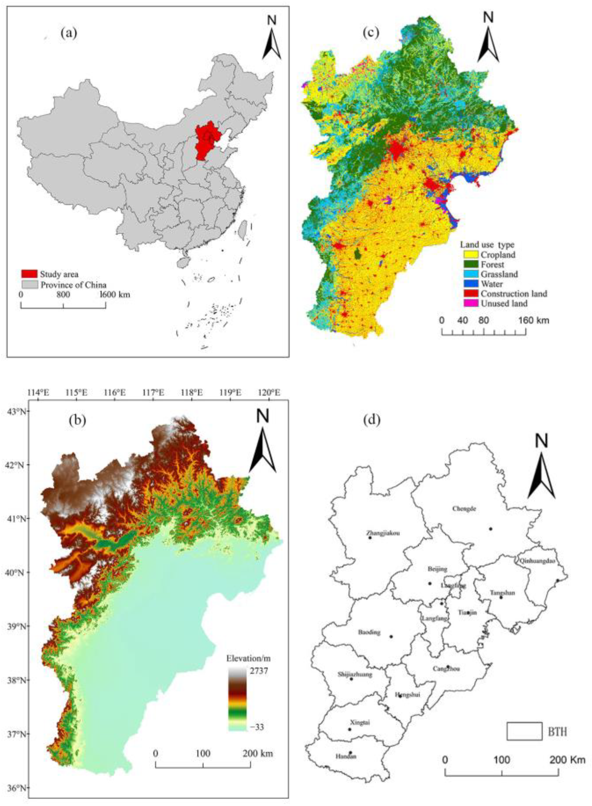
2.1. Study Area
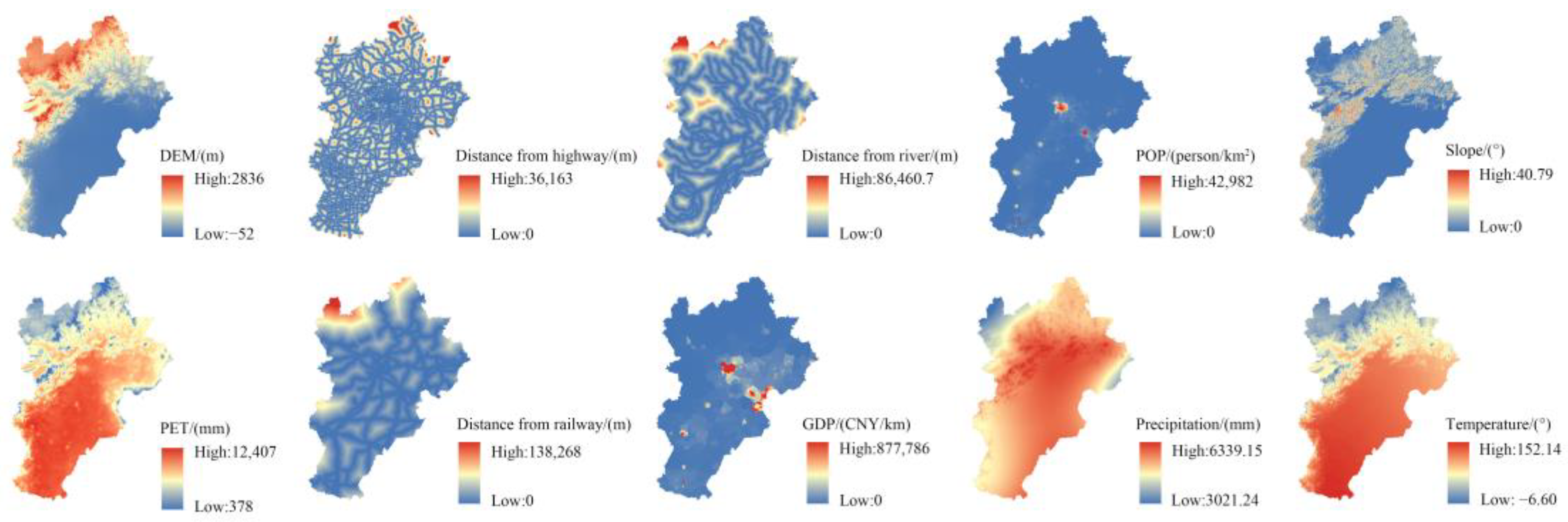
2.2. Data Sources
2.3. Ecosystem Service Assessment Methods
2.3.1. Ecosystem Service Assessment
2.3.2. Carbon Stock
2.3.3. Water Yield
2.3.4. Habitat Quality
2.3.5. Soil Conservation
2.3.6. PLUS Model
2.3.7. Correlation Analysis
2.3.8. Bivariate Spatial Autocorrelation
3. Results
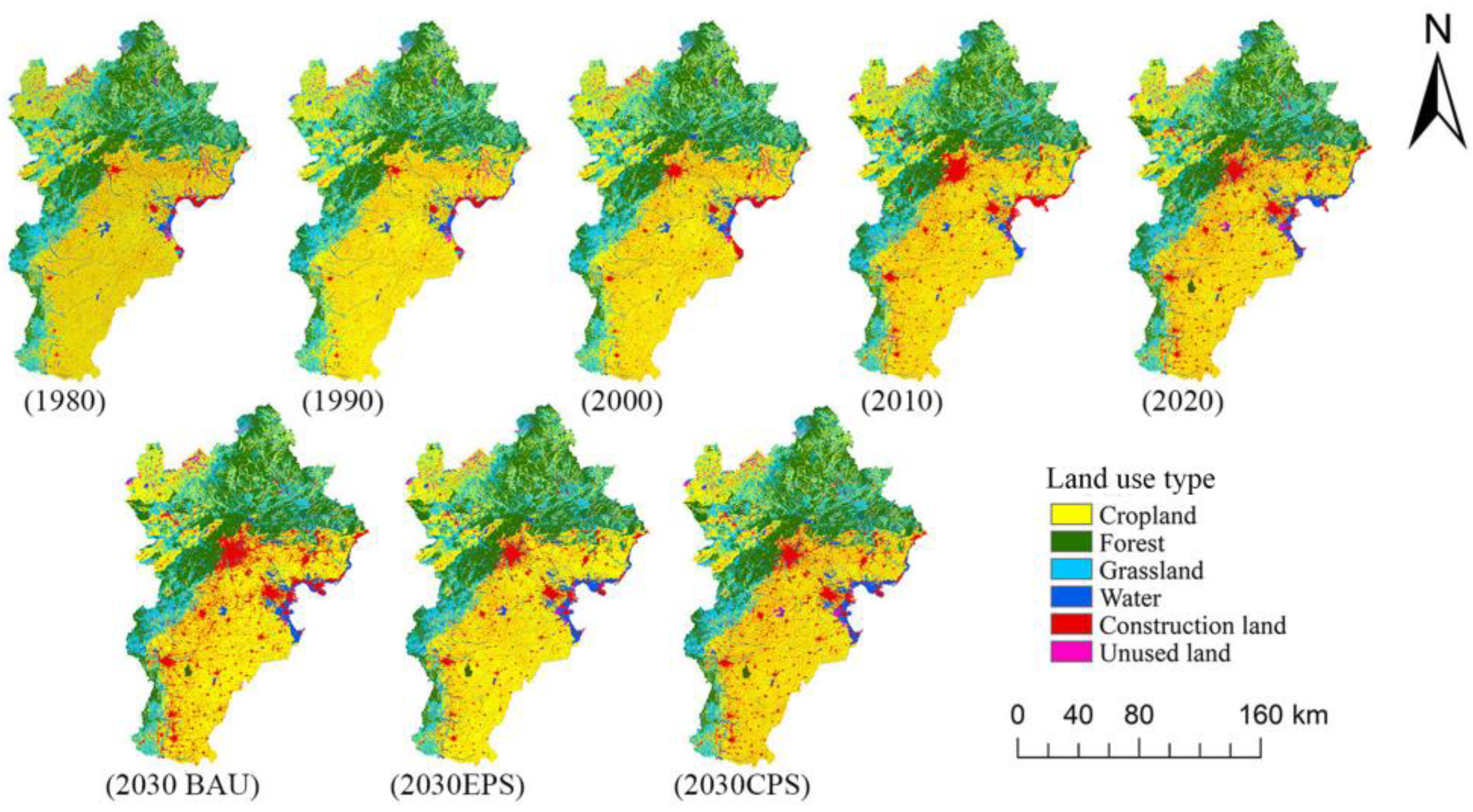
3.1. Land Use Changes during 1980–2020
3.2. Changes in Ecosystem Services during 1980–2020
3.3. Future Changes in Land Use and Services under Three Different Simulation Scenario
3.3.1. Land Use Changes under Three Scenarios in 2030
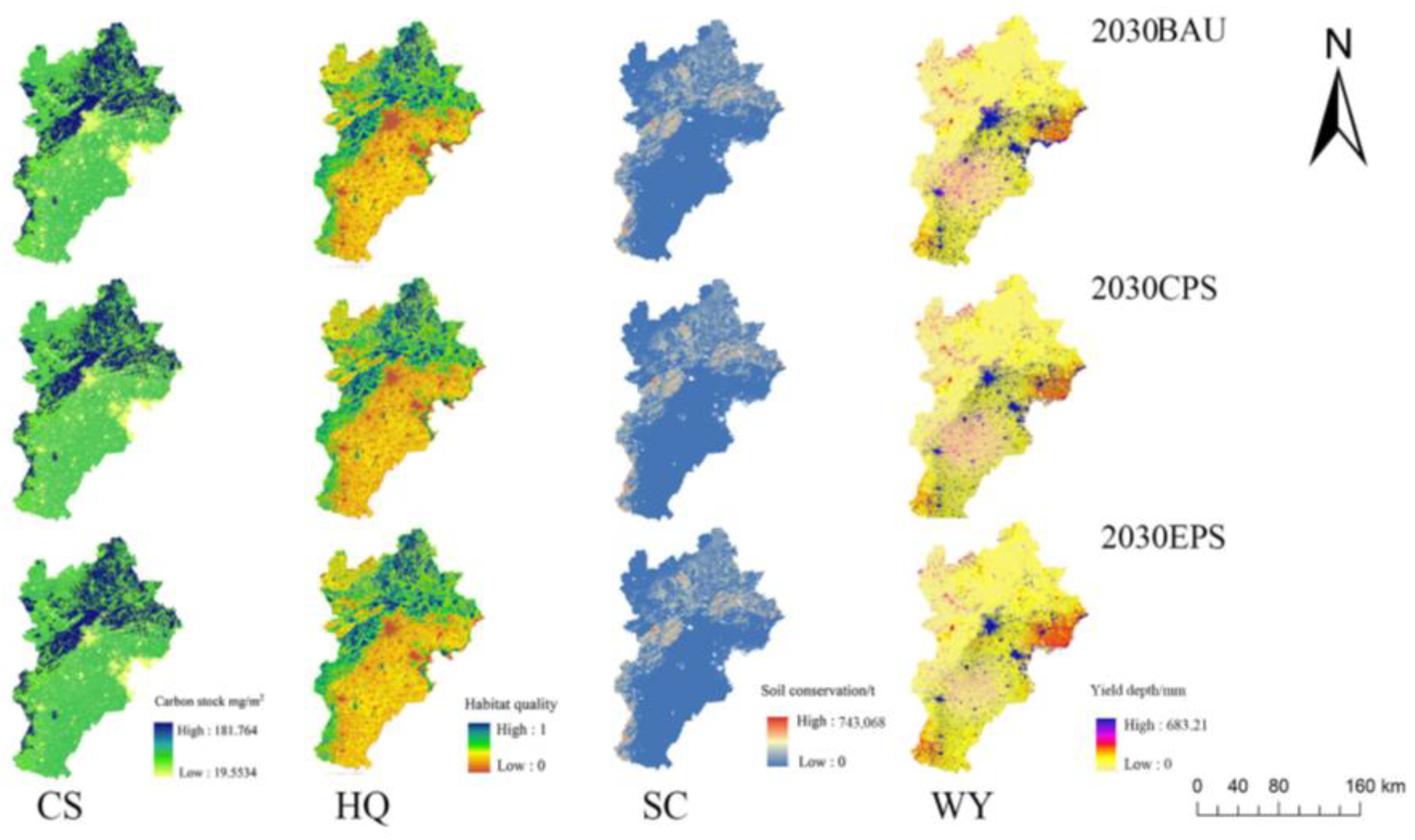
3.3.2. Changes in Ecosystem Services under Three Different Scenarios in 2030
3.4. Ecosystem Service Trade-off and Synergy
3.4.1. Temporal Changes in Ecosystem Trade-off/Synergy Relationships
3.4.2. Spatial Variation in Ecosystem Trade-Offs/Synergies
4. Discussion
4.1. Comparison of Ecosystem Services
4.2. Trade-Offs and Synergies of Ecosystem Services
4.3. Limitations and Perspectives
5. Conclusions
Author Contributions
Funding
Institutional Review Board Statement
Informed Consent Statement
Data Availability Statement
Conflicts of Interest
References
- Adrián, L.; Pilar, M.; Carlos, T. Spatial configuration of patches with different ecological maturity: Implications for service supply at the landscape level. J. Environ. Manag. 2023, 342, 118094. [Google Scholar]
- Li, F.; Liu, H.; Wu, S.; Wang, Y.; Xu, Z.; Yu, P.; Yan, D. A PES framework coupling socioeconomic and ecosystem dynamics from a sustainable development perspective. J. Environ. Manag. 2023, 329, 117043. [Google Scholar] [CrossRef]
- Li, Q.; Li, W.; Wang, S.; Wang, J. Assessing heterogeneity of trade-offs/synergies and values among ecosystem services in Beijing-Tianjin-Hebei urban agglomeration. Ecol. Indic. 2022, 140, 109026. [Google Scholar] [CrossRef]
- Sun, Y.; Ren, Z.; Hao, M.; Duan, Y. Spatial and temporal changes in the synergy and trade-of between ecosystem services, and its influencing factors in Yanan, Loess Plateaul. Acta Ecol. Sin. 2019, 39, 3443–3454. [Google Scholar]
- Ma, S.; Qiao, Y.; Wang, L.; Zhang, J. Terrain gradient variations in ecosystem services of different vegetation types in mountainous regions: Vegetation resource conservation and sustainable development. For. Ecol. Manag. 2021, 482, 118856. [Google Scholar] [CrossRef]
- Zhang, X.; Jin, X.; Liang, X.; Ren, J.; Han, B.; Liu, J.; Fan, Y.; Zhou, Y. Implications of land sparing and sharing for maintaining regional ecosystem services: An empirical study from a suitable area for agricultural production in China. Sci. Total Environ. 2022, 820, 153330. [Google Scholar] [CrossRef] [PubMed]
- Fang, Z.; Ding, T.; Chen, J.; Xue, S.; Zhou, Q.; Wang, Y.; Wang, Y.; Huang, Z.; Yang, S. Impacts of land use/land cover changes on ecosystem services in ecologically fragile regions. Sci. Total Environ. 2022, 831, 154967. [Google Scholar] [CrossRef]
- Stosch, K.; Quilliam, R.; Bunnefeld, N. Quantifying stakeholder understanding of an ecosystem service trade-off. Sci. Total Environ. 2019, 651, 2524–2534. [Google Scholar] [CrossRef]
- Aryal, K.; Maraseni, T.; Apan, A. How much do we know about trade-offs in ecosystem services? A systematic review of empirical research observations. Sci. Total Environ. 2022, 806, 151229. [Google Scholar] [CrossRef]
- Hua, F.; Bruijnzeel, L.; Me, L. The biodiversity and ecosystem service contributions and trade-offs of forest restoration approaches. Science 2022, 376, 839–844. [Google Scholar] [CrossRef]
- Guo, A.; Niu, L.; Liu, P.; Li, Y. Carbon emission from land use in urban agglomeration of the Yellow River basin. Econ. Geogr. 2023, 43, 172–178+240. [Google Scholar]
- Li, T.; Li, W.; Qian, Z. Variations in ecosystem service value in response to land use changes in Shenzhen. Ecol. Econ. 2008, 69, 1427–1435. [Google Scholar]
- Xie, W.; Huang, Q.; He, C.; Zhao, X. Projecting the impacts of urban expansion on simultaneous losses of ecosystem services: A case study in Beijing, China. Ecol. Indic. 2018, 84, 183–193. [Google Scholar] [CrossRef]
- Chen, X.; Wang, T.; Li, B. Scenario simulation of future land use and ecosystem service change in ecological conservation area of northwest Beijing. J. Northwest For. Coll. 2021, 36, 86–95. [Google Scholar]
- Yang, S.; Zhao, W.; Liu, Y. Influence of land use change on the ecosystem service trade-offs in the ecological restoration area: Dynamics and scenarios in the Yanhe watershed, China. Sci. Total Environ. 2018, 644, 556–566. [Google Scholar] [CrossRef] [PubMed]
- Gong, J.; Liu, D.; Zhang, J.; Xie, Y.; Cao, E.; Li, H. Tradeoffs/synergies of multiple ecosystem services based on land use simulation in a mountain-basin area, western China. Ecol. Indic. 2019, 99, 283–293. [Google Scholar] [CrossRef]
- Shen, J.; Li, S.; Wang, H.; Wu, S.; Liang, Z.; Zhang, Y.; Wei, F.; Li, S.; Ma, L.; Wang, Y.; et al. Understanding the spatial relationships and drivers of ecosystem service supply-demand mismatches towards spatially-targeted management of social-ecological system. J. Clean. Prod. 2023, 406, 136882. [Google Scholar] [CrossRef]
- Zhang, D.; Nan, Y.; Zhu, W.; He, C.; Liu, Z.; Yang, Y. Indirect impacts of future urban expansion on ecosystem services in the transnational area of China, North Korea, and Russia. Land Degrad. Dev. 2023, 34, 2334–2348. [Google Scholar] [CrossRef]
- Li, X.; Chen, C.; Li, K. Multi-scenario simulation of land use in Yan’an City based on Markov-PLUS model. J. Inn. Mong. Norm. Univ. 2024, 53, 153–162. [Google Scholar]
- Liang, X.; Guan, Q.; Clarke, K.; Liu, S.; Wang, B.; Yao, Y. Understanding the drivers of sustainable land expansion using a patch-generating land use simulation (PLUS) model: A case study in Wuhan, China. Comput. Environ. Urban Syst. 2021, 85, 101569. [Google Scholar] [CrossRef]
- Zhao, H.; Liu, H.; Yang, Z.; Liu, X.; Miao, Q.; Fu, H. Ecosystem services assessment and multi-scenario prediction in Liaoning province from 2000 to 2020. Environ. Sci. 2023, 45, 4137–4151. [Google Scholar]
- Lin, M.; Liu, H.; Zhou, R.; Gong, J. Evaluation and trade-offs of ecosystem services in the Guangdong-Hong Kong-Macao Greater Bay Area under multi-scenario simulation. Geogr. Res. 2021, 40, 2657–2669. [Google Scholar]
- Ning, L.; Liang, X.; Cheng, C. Ecosystem health assessment and spatiotemporal changes in the Beijing-Tianjin-Hebei region. Chin. J. Ecol. Sci. 2018, 40, 1–12. [Google Scholar]
- Li, D.; Wu, S.; Liu, L.; Liang, Z.; Li, S. Evaluating regional water security through a freshwater ecosystem service flow model: A case study in Beijing-Tianjin-Hebei region, China. Ecol. Indic. 2017, 81, 159–170. [Google Scholar] [CrossRef]
- Xie, H.; He, Y.; Xie, X. Exploring the factors influencing ecological land change for China’s Beijing–Tianjin–Hebei Region using big data. J. Clean. Prod. 2016, 142, 677–687. [Google Scholar] [CrossRef]
- Ma, Z.; Xie, H.; Lin, L.; Hu, Q.; Qian, Y.; Zhang, S.; Wang, G.; Li, J.; Tan, C.; Guo, H.; et al. The environmental geological conditions of Land resources in the Beijing-Tianjin-Hebei region. Geol. China 2017, 44, 857–873. [Google Scholar]
- Ji, J.; Xiong, Y.; Jiang, L.; Zhang, W.; Chen, D.; Du, J.; Liu, W. Study on the evaluation of geological disaster susceptibility of Jing -Jin- Ji urban agglomeration based on geodetector and spatial principal component analysis methods. J. Catastrophology 2023, 38, 94–99. [Google Scholar]
- Wang, L.; Dong, L.; Zhao, Z.; Lu, S.; Wang, J.; Liu, Y.; Jim, S.; Guan, H.; Guo, K. Vegetation diversity and mapping in the priority area of Taihang Mountains biodiversity conservation (Beijing-Tianjin-Hebei region). Sci. Sin. Vitae 2021, 51, 289–299. [Google Scholar] [CrossRef]
- Zhong, Y.; Zou, Y.; Wang, S.; Li, L.; Li, R.; Xiao, N.; Chem, F. Investigation and analysis of the species and community diversity of insects in different types of habitats in Beijing-Tianjin-Hebei area of Taihang Mountain. J. Environ. Entomol. 2023, 45, 285–292. [Google Scholar]
- Zhou, X.; Huang, Z.; Zhang, X.; Xing, S. Protection of natural vegetation and distribution of nature reserves in Being-Tianjin-Hebei region. Ecol. Sci. 2017, 36, 64–71. [Google Scholar]
- Yang, M.; Gao, X.; Zhao, X.; Wu, P. Scale effect and spatially explicit drivers of interactions between ecosystem services: A case study from the Loess Plateau. Sci. Total Environ. 2021, 785, 147389. [Google Scholar] [CrossRef]
- Wu, W.; Xu, L.; Zheng, H.; Zhang, X. How much carbon storage will the ecological space leave in a rapid urbanization area? Scenario analysis from Beijing-Tianjin-Hebei Urban Agglomeration. Resour. Conserv. Recycl. 2023, 189, 106744. [Google Scholar] [CrossRef]
- Gong, S.; Zhang, Y.; Li, Y. Change and prediction of carbon storage in Beijing-Tianjin-Hebei region based on PLUS-InVEST mode. J. Arid Land Resour. Environ. 2023, 37, 20–28. [Google Scholar]
- Wang, Z.; Xu, D.; Peng, D.; Zhang, X. Future climate change would intensify the water resources supply-demand pressure of afforestation in inner Mongolia, China. J. Clean. Prod. 2023, 407, 137145. [Google Scholar] [CrossRef]
- Ning, T.; Feng, Q.; Li, Z.; Li, Z.; Xi, H.; Yang, L. Precipitation changes and its interaction with terrestrial water storage determine water yield variability in the world’s water towers. Sci. Total Environ. 2023, 880, 163285. [Google Scholar] [CrossRef] [PubMed]
- Sun, X.; Jiang, Z.; Liu, F.; Zhang, D. Monitoring spatio-temporal dynamics of habitat quality in Nansihu Lake basin, eastern China, from 1980 to 2015. Ecol. Indic. 2019, 102, 716–723. [Google Scholar] [CrossRef]
- Feng, Z.; Jin, X.; Chen, T.; Wu, J. Understanding trade-offs and synergies of ecosystem services to support the decision-making in the Beijing–Tianjin–Hebei region. Land Use Policy 2021, 106, 105446. [Google Scholar] [CrossRef]
- Bace, R.; Hofmeister, J.; Vitkova, L.; Brabec, M.; Begovic, K.; Cada, V. Response of habitat quality to mixed severity disturbance regime in Norway spruce forests. J. Appl. Ecol. 2023, 14409, 1365–2664. [Google Scholar] [CrossRef]
- Yang, J.; Xie, B.; Zhang, D. The Trade-Offs and Synergistic Relationships between Grassland Ecosystem Functions in the Yellow River Basin. Diversity 2021, 13, 505. [Google Scholar] [CrossRef]
- Chen, W.; Wang, G.; Gu, T.; Fang, C.; Pan, S.; Zeng, J.; Wu, J. Simulating the impact of urban expansion on ecosystem services in Chinese urban agglomerations: A multi-scenario perspective. Environ. Impact Assess. Rev. 2023, 103, 107275. [Google Scholar] [CrossRef]
- Zhang, S.; Zhong, Q.; Cheng, D.; Xu, C.; Chang, Y.; Lin, Y.; Li, B. Coupling Coordination Analysis and Prediction of Landscape Ecological Risks and Ecosystem Services in the Min River Basin. Land 2022, 11, 222. [Google Scholar] [CrossRef]
- Ma, S.; Wang, H.; Wang, L.; Jiang, J.; Gong, J.; Wu, S.; Luo, G. Evaluation and simulation of landscape evolution and its ecological effects under vegetation restoration in the northern sand prevention belt, China. Catena 2022, 218, 106555. [Google Scholar] [CrossRef]
- Zheng, L.; Wang, Y.; Li, J. Quantifying the spatial impact of landscape fragmentation on habitat quality: A multi-temporal dimensional comparison between the Yangtze River Economic Belt and Yellow River Basin of China. Land Use Policy 2023, 125, 106463. [Google Scholar] [CrossRef]
- Lu, C.; Cai, X.; Hao, C. Ecosystem service tradeoff and synergistic relationship in the Yellow River Delta High-Efficiency Eco-Economic Zone. Chin. J. Appl. Ecol. 2024, 35, 457–468. [Google Scholar]
- Li, S.; Yang, H.; La, M.; Liu, J.; Lei, G. Impacts of Land-Use and Land-Cover Changes on Water Yield: A Case Study in Jing-Jin-Ji, China. Sustainability 2018, 10, 960. [Google Scholar] [CrossRef]
- Liu, H.; Xiao, W.; Li, Q. Spatial and temporal changes and tradeoffs of ecosystem services in Beijing. Chin. J. Ecol. 2021, 40, 209–219. [Google Scholar]
- Zhang, P.; Liu, S.; Zhou, Z.; Liu, C.; Xu, L.; Gao, X. Supply and demand measurement and spatio-temporal evolution of ecosystem services in Beijing-Tianjin-Hebei Region. Acta Ecol. Sin. 2021, 41, 3354–3367. [Google Scholar]
- Wang, S.; Li, Y.; Li, Q.; Hu, S.; Wang, J.; Li, W. Water and soil conservation and their trade-off and synergistic relationship under changing environment in Zhangjiakou-Chengde area. Acta Ecol. Sin. 2022, 42, 5391–5403. [Google Scholar]
- Rodriguez-Lloveras, X.; Buytaert, W.; Benito, G. Land use can offset climate change induced increases in erosion in Mediterranean watersheds. Catena 2016, 143, 244–255. [Google Scholar] [CrossRef]
- Li, J.; Zhang, C.; Zhu, S. Relative contributions of climate and land-use change to ecosystem services in arid inland basins. J. Clean. Prod. 2021, 298, 126844. [Google Scholar] [CrossRef]
- Qiu, J.; Huang, T.; Yu, D. Evaluation and optimization of ecosystem services under different land use scenarios in a semiarid landscape mosaic. Ecol. Indic. 2022, 135, 108516. [Google Scholar] [CrossRef]
- Fu, Q.; Li, B.; Hou, Y.; Xu, B.; Zhang, X. Effects of land use and climate change on ecosystem services in Central Asia′s arid regions: A case study in Altay Prefecture, China. Sci. Total Environ. 2017, 607, 633–646. [Google Scholar] [CrossRef] [PubMed]
- Ren, Y.; Liu, X.; Xu, X.; Sun, S.; Zhao, L.; Liang, X.; Zeng, L. Multi-scenario simulation of land use change and its impact on ecosystem services in Beijing-Tianjin-Hebei region based on the FLUS-InVEST Model. Acta Ecol. Sin. 2023, 43, 4473–4487. [Google Scholar]
- Yu, X.; LV, C.; Guo, X.; Zhang, Z.; Li, S.; Hao, J. Assessment of land ecological status in Beijing-Tianjin-Hebei city cluster. China Land Sci. 2018, 32, 89–96. [Google Scholar]
- Srichaichana, J.; Trisurat, Y.; Ongsomwang, S. Land use and land cover scenarios for optimum water yield and sediment retention ecosystem services in Klong UTapao watershed, Songkhla, Thailand. Sustainabllity 2019, 11, 2895. [Google Scholar] [CrossRef]
- Guo, Z.; Yan, Z.; He, R.; Yang, H.; Ci, H.; Wang, R. Impacts of Land Use Conversion on Soil Erosion in the Urban Agglomeration on the Northern Slopes of the Tianshan Mountains. Land 2024, 13, 550. [Google Scholar] [CrossRef]
- Zhang, J.; Zhu, W.; Zhu, L.; Li, Y. Multiscale analysis of forest ecosystem service trade-offs/synergies in Funiu Mountain region. Acta Geogr. Sin. 2020, 75, 975–988. [Google Scholar]
- He, J.; Shi, X.; Fu, Y.; Yuan, Y. Spatiotemporal pattern of the trade-offs and synergies of ecosystem services after Grain for Green Program: A case study of the Loess Plateau, China. Environ. Sci. Pollut. Res. 2020, 27, 30020–30033. [Google Scholar] [CrossRef]


| Dataset | Data Source | Resolution | Time |
|---|---|---|---|
| Land Use | GlobeLand30 data center (http://www.globallandcover.com/); accessed on 1 March 2023 | 30 m | 1980, 1990, 2000, 2010, 2020 |
| DEM | GlobeLand30 data center (http://www.globallandcover.com/); accessed on 1 March 2023 | 30 m | 1980, 1990, 2000, 2010, 2020 |
| Slope | Geospatial Data Cloud (http://www.gscloud.cn/); accessed on 1 March 2023 | 30 m | 1980, 1990, 2000, 2010, 2020 |
| Temperature | China Meteorological Data Service Centre (http://data.cma.cn/); accessed on 1 March 2023 | 1 km | 1980, 1990, 2000, 2010, 2020 |
| Precipitation | China Meteorological Data Service Centre (http://data.cma.cn/); accessed on 1 March 2023 | 1 km | 1980, 1990, 2000, 2010, 2020 |
| Evapotranspiration | China Science Data Center for Resources and Environment (http://www.resdc.cn/); accessed on 1 March 2023 | 1 km | 1980, 1990, 2000, 2010, 2020 |
| Soil texture | China Science Data Center for Resources and Environment (http://www. resdc.cn/); accessed on 1 March 2023 | 1 km | 1980, 1990, 2000, 2010, 2020 |
| Soil root depth | China Soil Dataset from World Soil Database (HWSD) (https://westdc.westgis.ac.cn); accessed on 1 March 2023 | 1 km | 1980, 1990, 2000, 2010, 2020 |
| Plant available water content | Cold and Arid Regions Sciences Data Center (http://westdc. westgis.ac.cn/); accessed on 1 March 2023 | 1 km | 1980, 1990, 2000, 2010, 2020 |
| Population density | National Earth System Science Data Center (http://www.geodata.cn/); accessed on 1 March 2023 | 1 km | 2020 |
| GDP | China Science Data Center for Resources and Environment (https://www.resdc.cn/); accessed on 1 March 2023 | 1 km | 2020 |
| River data | National Geographical Information Resource Catalog Service System (https://www.webmap.cn/); accessed on 1 March 2023 | 1 km | 1980, 1990, 2000, 2010, 2020 |
| Distance from railways | OpenStreetMap (https://www.openstreetmap.org/); accessed on 1 March 2023 | Vector | 2020 |
| Distance from highways | OpenStreetMap (https://www.openstreetmap.org/); accessed on 1 March 2023 | Vector | 2020 |
| Distance from rivers | National Earth System Science Data Center (http://www.geodata.cn/); accessed on 1 March 2023 | Vector | 2020 |
| Land Use Type | Above-Ground Biomass | Below-Ground Biomass | Soil |
|---|---|---|---|
| Cropland | 3.20 | 0.30 | 112.90 |
| Forestland | 69.60 | 21.00 | 133.80 |
| Grassland | 1.18 | 13.60 | 60.50 |
| Water | 3.40 | 12.10 | 8.64 |
| Construction land | 0.40 | 6.90 | 28.80 |
| Unused land | 9.13 | 1.82 | 34.08 |
| Land Use Type | Habitat Suitability | Threat Factors | ||
|---|---|---|---|---|
| Cropland | Construction Land | Unused Land | ||
| Cropland | 0.30 | 0.00 | 0.70 | 0.20 |
| Forestland | 1.00 | 0.60 | 0.80 | 0.30 |
| Grassland | 0.90 | 0.50 | 0.60 | 0.40 |
| Water | 0.75 | 0.60 | 0.65 | 0.30 |
| Construction land | 0.00 | 0.00 | 0.00 | 0.00 |
| Unused land | 0.10 | 0.10 | 0.20 | 0.00 |
| Land Use | Cropland | Forestland | Grassland | Water | Construction Land | Unused Land |
|---|---|---|---|---|---|---|
| Weight | 0.49 | 0.15 | 0.03 | 0.16 | 0.18 | 0.05 |
| BAU | CPS | EPS | ||||||||||||||||
|---|---|---|---|---|---|---|---|---|---|---|---|---|---|---|---|---|---|---|
| A | B | C | D | E | F | A | B | C | D | E | F | A | B | C | D | E | F | |
| A | 1 | 1 | 1 | 1 | 1 | 1 | 1 | 0 | 0 | 0 | 0 | 0 | 1 | 1 | 1 | 0 | 0 | 0 |
| B | 1 | 1 | 1 | 1 | 1 | 1 | 1 | 1 | 1 | 0 | 0 | 0 | 0 | 1 | 0 | 0 | 0 | 0 |
| C | 1 | 1 | 1 | 1 | 1 | 1 | 1 | 1 | 1 | 1 | 0 | 0 | 0 | 1 | 1 | 0 | 0 | 0 |
| D | 1 | 1 | 1 | 1 | 1 | 1 | 1 | 0 | 0 | 1 | 0 | 0 | 0 | 1 | 1 | 1 | 0 | 0 |
| E | 1 | 1 | 1 | 1 | 1 | 1 | 0 | 0 | 0 | 0 | 1 | 1 | 1 | 1 | 1 | 1 | 1 | 0 |
| F | 1 | 1 | 1 | 1 | 1 | 1 | 1 | 0 | 0 | 0 | 0 | 1 | 0 | 1 | 1 | 1 | 0 | 1 |
| Year | Cropland | Forestland | Grassland | Water | Construction Land | Unused Land |
|---|---|---|---|---|---|---|
| 1980 | 113,036.58 | 45,208.89 | 35,465.04 | 6356.97 | 14,215.59 | 2274.48 |
| 1990 | 112,696.79 | 44,788.77 | 35,831.43 | 6262.47 | 14,714.46 | 2261.70 |
| 2000 | 109,343.54 | 44,678.92 | 35,304.81 | 6335.28 | 17,814.55 | 2074.06 |
| 2010 | 104,024.45 | 45,006.18 | 34,063.52 | 5455.45 | 25,984.91 | 1293.16 |
| 2020 | 99,904.59 | 45,938.66 | 34,053.74 | 6801.00 | 27,450.09 | 1665.59 |
| 2030 BAU | 99,508.96 | 46,159.32 | 34,078.50 | 6337.74 | 28,915.86 | 1551.80 |
| 2030 CPS | 100,850.60 | 46,767.24 | 34,102.61 | 6625.40 | 27,131.99 | 1535.08 |
| 2030 EPS | 104,754.84 | 47,834.89 | 34,965.89 | 6871.15 | 20,154.55 | 1251.60 |
Disclaimer/Publisher’s Note: The statements, opinions and data contained in all publications are solely those of the individual author(s) and contributor(s) and not of MDPI and/or the editor(s). MDPI and/or the editor(s) disclaim responsibility for any injury to people or property resulting from any ideas, methods, instructions or products referred to in the content. |
© 2024 by the authors. Licensee MDPI, Basel, Switzerland. This article is an open access article distributed under the terms and conditions of the Creative Commons Attribution (CC BY) license (https://creativecommons.org/licenses/by/4.0/).
Share and Cite
Gong, S.; Zhang, Y.; Pu, X.; Wang, X.; Zhuang, Q.; Bai, W. Assessing and Predicting Ecosystem Services and Their Trade-Offs/Synergies Based on Land Use Change in Beijing–Tianjin–Hebei Region. Sustainability 2024, 16, 5609. https://doi.org/10.3390/su16135609
Gong S, Zhang Y, Pu X, Wang X, Zhuang Q, Bai W. Assessing and Predicting Ecosystem Services and Their Trade-Offs/Synergies Based on Land Use Change in Beijing–Tianjin–Hebei Region. Sustainability. 2024; 16(13):5609. https://doi.org/10.3390/su16135609
Chicago/Turabian StyleGong, Shengxuan, Yuhu Zhang, Xiao Pu, Xiaohan Wang, Qiuyu Zhuang, and Wenhui Bai. 2024. "Assessing and Predicting Ecosystem Services and Their Trade-Offs/Synergies Based on Land Use Change in Beijing–Tianjin–Hebei Region" Sustainability 16, no. 13: 5609. https://doi.org/10.3390/su16135609