Article

Investigating the Impact of Recent and Future Urbanization on Flooding in an Indian River Catchment

by
Sonu Thaivalappil Sukumaran
1,* and
Stephen J. Birkinshaw
2
1
Arup, 12 Wellington Pl, Leeds LS1 4AP, UK
2
School of Engineering, Newcastle University, Newcastle upon Tyne NE1 7RU, UK
*
Author to whom correspondence should be addressed.
Sustainability 2024, 16(13), 5652; https://doi.org/10.3390/su16135652 (registering DOI)
Submission received: 24 April 2024 / Revised: 25 June 2024 / Accepted: 27 June 2024 / Published: 2 July 2024
(This article belongs to the Special Issue Sustainability in Urban Climate Change and Ecosystem Services)

Abstract

:
Socioeconomic growth in India has caused massive infrastructure development which has resulted in extensive damage to the natural environment. A consequence of this urbanization has been extensive monsoon flooding in many locations within the country. The impact of recent land use and land cover (LULC) change because of urbanization and a series of future LULC scenarios is assessed for the Meenachil river basin in central Kerala, India. This catchment flows into the Kuttanad administrative area, which has the country’s lowest elevation, an increasing population, and currently suffers from regular flooding. Hydrological modeling using SHETRAN and hydraulic modeling using HEC-RAS predicts that an extreme event will produce a 105% rise in flood depth in 2100 compared to 2005. A scenario that incorporates Nature-based Solutions suggests the rise in flood depth could be reduced by 44%. A catchment response for future development is needed but is hindered by different administrative boundaries within the river basins that flow into the Kuttanad administrative area, and so this study concludes by providing regional-scale planning recommendations that integrate hydrologic components.

1. Introduction

The change in land use and land cover (LULC) from agricultural land and forests to an urban environment is among the most significant human influences [1,2]. This shift has a major impact on catchment water balances, primarily due to the introduction of impermeable surfaces, the loss of deep-rooted vegetation, and the modification of drainage networks [3,4]. These impacts are further exacerbated by extreme rainfall events, which are becoming increasingly common. When the rate of precipitation exceeds the maximum infiltration capacity of the soil, the surplus precipitation rapidly flows over the land surface towards stream channels, contributing significantly to soil erosion and flooding. Urbanization trends and the associated increases in impermeable surfaces are contributing to frequent flooding events worldwide, including in India, where urban populations are steadily growing [5,6,7]. Although India’s population is predominantly rural, the number of people living in an urban environment is increasing and today constitutes more than 30% of the total population of the country [8]. Census data from Kerala, a state in the southernmost end of India, also reveal an increase in urbanization [9] as a result of accelerated socioeconomic growth. Within Kerala, the Kuttanad Wetland System (KWS) has similar growth and urbanization issues as the rest of the state and country and is considered as a case study in this work along with the Meenachil river catchment, which is one of five major catchments that drain into the KWS.
The traditional approach of addressing urban development issues in developing countries by confining them to political boundaries has only exacerbated flooding issues. The future calls for a holistic approach that adopts measures at the catchment scale. However, access to accurate datasets is difficult in developing nations, unlike in developed nations such as the United Kingdom [10] and the United States [11] where there are reliable long-term stream flow and rainfall records. This makes investigations into the impact of LULC change on catchments in developing countries like India challenging and only a few studies have attempted to attribute changes in the water balance and flooding issues to LULC and associate them with catchment planning [12,13].
Hydrological modeling can be used to study the effect of LULC on flows in river catchments by running different scenarios, including potential future LULC scenarios. One approach is the implementation of physically based spatially distributed (PBSD) models, where land use characteristics are precisely represented, and all processes affected by them are simulated using physically estimable parameters [14,15]. Models of this type to assess the impact of LULC on flow regimes include the SWAT model [16,17,18], MIKE-SHE, MIKE-11 [19], and SHETRAN [20,21]. These models take inputs such as LULC maps, soil maps, and weather data to generate the corresponding surface runoff [18,19]. Ref. [22] reflected in their study that the capacity of a hydrological model to provide accurate forecasts depends on having carried out sufficient sensitivity analysis and model calibration.
Hydraulic computer models can be used to consider river flooding in more detail than hydrological models as they generally have a much finer grid resolution. Using river flow data from hydrological models as the input, flooded areas and depths along a floodplain can be comprehensively modeled. There are many existing hydraulic models which can be used, and these include HEC-RAS, InfoWORKS, MIKE11, etc. [23]. HEC-RAS has been applied for assessing and visualizing river dynamics by running 1D steady and 2D unsteady river flow simulations to estimate floods, and for predicting the extent of floods, simulating direct runoff, and analyzing huge floodplains [23,24]. Similarly, MIKE 11 offers a combined 1D–2D hydrodynamic model for the forecasting, mapping and analysis of floods, [24]. InfoWORKS is a GIS-based hydrologic, hydraulic, and water quality simulation model primarily used for managing storm, sanitary, and sewage networks [25].
To mitigate flooding, grey infrastructure such as dikes have traditionally been the most common approach [26]. However, these structures have a limited threshold and an inherent failure probability. Paradoxically, the safety provided by dikes often leads to the increased use of flood-prone land, resulting in higher flood sensitivity and risk. As an alternative, Nature-based Solutions (NBSs) or hybrid solutions are increasingly recognized as cost-effective methods for flood risk control [27]. These solutions can take various forms, including soil restoration, tree planting, temporary storage ponds, and wetlands [28]. The main goal of implementing NBSs is to reduce downstream flood risk by attenuating river flow and prolonging the response time to upstream rainfall. NBSs also contribute to reducing the risk of both floods and droughts by promoting water infiltration into aquifers, resulting in prolonged baseflow availability [29]. While these measures cannot completely prevent floods, they can significantly mitigate their negative impacts and offer additional advantages such as improved water quality, tourism opportunities, and soil erosion management.
The aim of this work is to use the SHETRAN hydrological model and the HEC-RAS hydraulic model to answer three questions:
(1).
What is the impact of recent urbanization and potential future urbanization on flooding in the Meenachil river catchment and the Kuttanad administrative area in central Kerala, India?
(2).
How much benefit will NBSs provide in reducing the flooding risk?
(3).
What regional-scale planning recommendations are needed to minimize the flood risk in the Kuttanad administrative area under future developments?

2. Materials and Methods

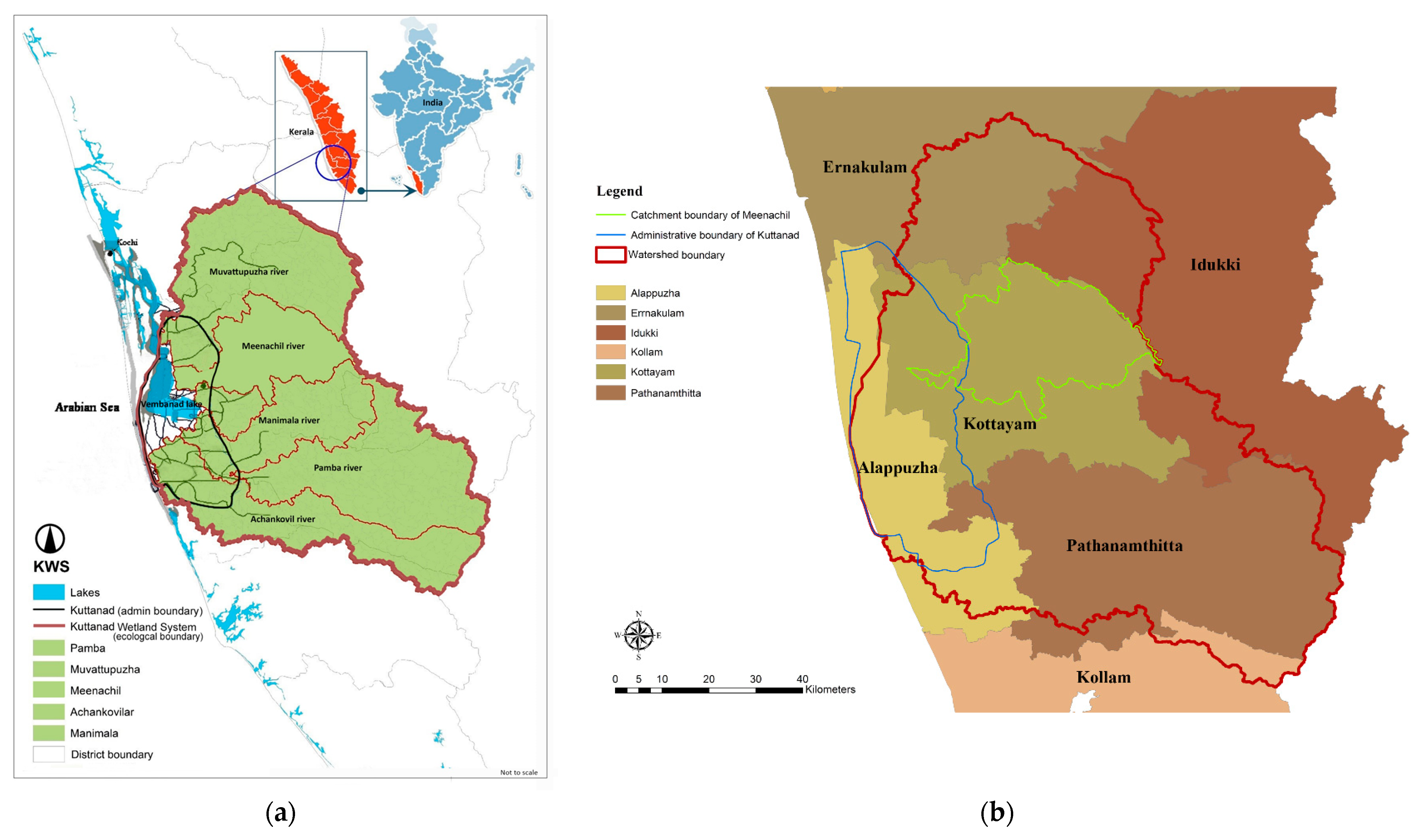
2.1. Kuttanad Wetland System

The Kuttanad Wetland System, Kerala, the lowest point in India lying 2–3 m below the mean sea level [30], is better known as the rice bowl of Kerala [25] and is considered to be one of the country’s most severely vulnerable wetland systems. Together with the Vembanad lake, it is the second largest wetland system in the country (Figure 1a) [31]. There has been extensive land reclamation over many years due to population pressure, with a current density of 700 people per square km which is 40% greater than the Indian national average of 425 people per square km. According to a recent assessment by the Intergovernmental Panel on Climate Change (IPCC) of the United Nations, surface temperatures have increased by around one degree Celsius compared to the average of the last century, increasing the frequency with which tropical storms occur over the Arabian Sea, resulting in more frequent and intense rainfall over Kuttanad [32]. As a consequence, flooding has become a recurring problem, which has resulted in the loss of life and property in the region. The Kerala floods of 2018, 2019, and 2020 incurred huge losses to the state of Kerala, with the death of 625 people, millions displaced, and an economic loss of INR 900 billion. The floods of 2018 submerged Kuttanad for about 78 days in flood waters [33]. The inhabitants of lower Kuttanad are so susceptible to floods that many have started migrating to the cities of the nearby Alappuzha and Kottayam districts (see Figure 1b), changing their livelihood from farming to non-agricultural and service industries, with over 6000 households abandoning their houses since the 2018 Kerala floods [34]. This change of occupation together with the increasing population has caused an increase in the built-up or urban area with a corresponding reduction in agricultural land.
Five main river basins flow into the Kuttanad administrative area (Figure 1a), Manimala, Pamba, Achankovil, Muvattupuzha, and Meenachil [16]. A significant issue in all these river basins is escalating unplanned urbanization which is affecting flooding in the downstream Kuttanad administrative area.

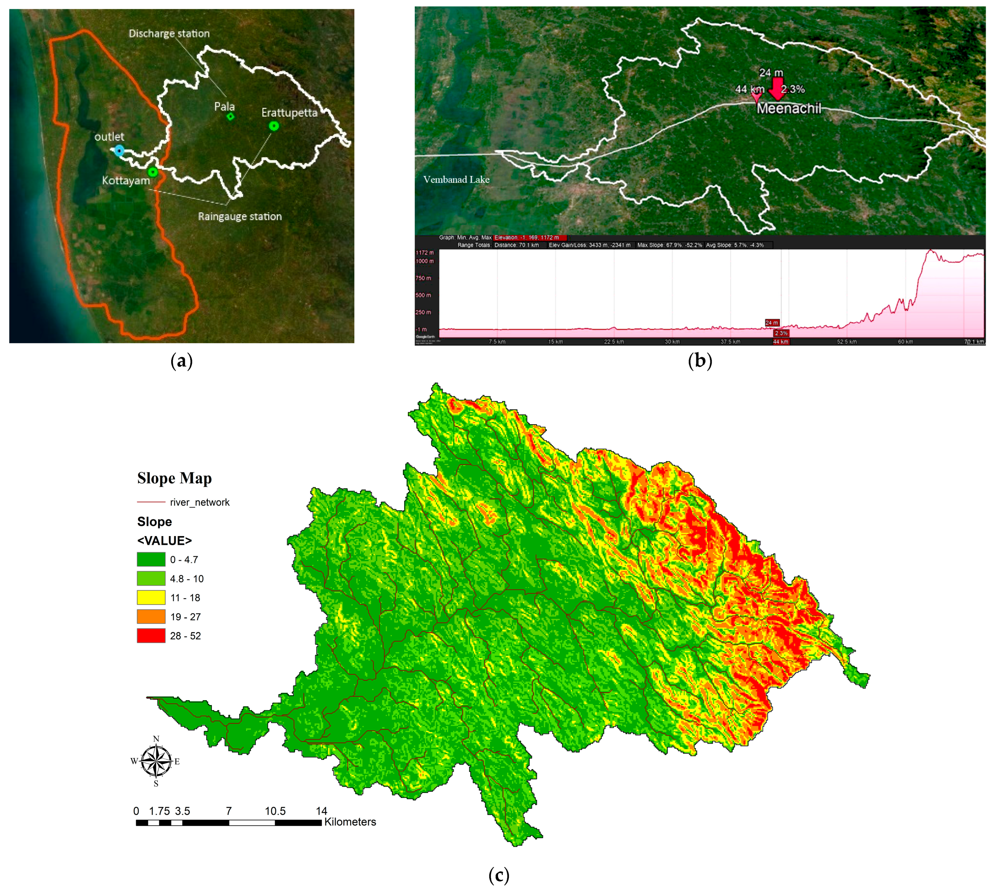
2.2. Meenachil River Basin and Data

Of the five river basins that flow into the Kuttanad administrative area (Figure 1a), the Meenachil river basin (854 km2) (Figure 2a) is the river basin most vulnerable to flooding due to its high population density, high elongation ratio, and low bifurcation ratio [16]. The Meenachil river basin is located between 9°32′2.79″ and 9°51′19.82″ N, and 76°29′29.95″ and 76°56′0.67″ E [35]. The basin lies within the administrative boundary of the Kottayam district (Figure 1b). The Meenachil river originates at Araikunnumudi in the Western Ghats at an elevation of 1182 m above the mean sea level (MSL) flowing down to 3.0 below the MSL and emptying into the KWS (Figure 2b). The 78 km long river is perennial in nature and is primarily fed by the southwest monsoon (June to August) and supplemented with the northeast monsoon (October to November) [35]. Flood history maps from the Kerala State Disaster Management Authority (KSDMA) were collected for the years 2018, 2019, and 2020.
The LULC maps of 2005 and 2011 (Figure 3a,b) were taken from BHUVAN, an Indian web-based utility, and were prepared by the Indian Space Research Organization (ISRO) [36]. The LULC for 2015 was obtained from the Kerala State Remote Sensing and Environment Centre (KSRSEC) and was the only available LULC map in the public domain. The overall accuracy of different LULC classes varies from 79% to 97% as cited by BHUVAN [36].
The LULC 2005 map shows that agriculture plantation constitutes the most widespread type of LULC class within the catchment, which was followed by built-up areas, barren lands, water, and forest cover. The two most significant changes between 2005 and 2015 (Table 1) are the reduction in agricultural lands from 739.9 km2 in 2005 to 567.1 km2 in 2015 and the increase in built-up or urban areas from 53.1 km2 in 2005 to 192.5 km2 in 2015. This alteration in agricultural practices has also damaged groundwater supplies due to the rise in the number of bore wells negatively impacting the region’s aquifers [37]. Another significant change is the increase in barren lands between 2005 and 2011. The district of Kottayam (within which this catchment is located) is the leading rubber producer in India and the majority of the agricultural land in this district is rubber plantations [38]. As with all other commodities, the cost of natural rubber is subject to commodity cycles [39]; as a result, the extraction price of natural rubber has varied. The upward trend in natural rubber rates began in 2005 and peaked in 2010 before steadily declining from 2011 onwards. Likewise, the percentage composition of rubber within the catchment changed, higher until 2010 and declining from 2011, which then increased the percentage of scrubland. This change is reflected in the form of an increase in barren lands in 2011 in the LULC for 2011 (See Figure 3b) because of the seasonal rubber replantation process.
All the LULC maps show the higher parts of the basin are mostly devoid of naturally occurring forests. In addition, the central part of the basin is now overpopulated and intensively farmed. This has rendered the ground incapable of retaining water [40]. Due to this, the flow regime has altered with more surface runoff and less stored water, resulting in droughts in the summer and flooding during the wet seasons. Much of the topsoil has also been carried away during floods. There is now a concern that the river will transform into a drain carrying away rainwater during the rainy season, and a trash dump during the summer [40].
As with all remotely sensed land cover maps, there are issues related to the accuracy of the maps [41], particularly, as we are considering the change in land use from two different sources which use different algorithms. However, they are the best available data and Figure 3 shows a consistently increasing pattern in the built-up area, which has the most significant effect on the modeling.
The soil map was obtained from the Kerala State Landuse Board (KSLB), and it was found that the basin has five main soil types which are mostly well drained and deep (Figure S1 and Table S2 in the Supplementary Materials). The upstream parts of the river basin were found to have clay soils with a lower conductivity than the majority of the basin, where the soil type was a gravelly clay in nature. As the upstream part of the basin is also steep, it means there is likely to be more surface runoff than found in the midstream and downstream [42].
The Shuttle Radar Topography Mission (SRTM) Digital Elevation Model (DEM) (90 m resolution) was used in this study as its vertical accuracy was found to be greater than ASTER (15 m resolution) [16]. It was extracted from the SWAT India Database. The slope map obtained from the elevation data is shown in Figure 2c and this is important when considering the best locations for rubber plantations.
Daily rainfall time series data and the discharge data for the basin were obtained from the Kerala State Department of Irrigation. This study utilized rainfall data from the upstream rainfall station (Erattupetta) and the downstream rainfall station (Kottayam) from 1 January 1994 to 31 December 2021, inclusive, and discharge data from the midstream station (Pala) from 1 January 2000 to 31 December 2015 (Figure 2a). There is no measured discharge at the catchment outlet (Figure 2a). Daily potential evapotranspiration (PET) data were not available for the catchment and monthly data extracted from a global dataset [43] were used. As PET in tropical locations does not fluctuate significantly on a daily basis [44], this was considered to be acceptable.

2.3. Future LULC Maps

A key aspect of this work is obtaining realistic future LULC maps for the Meenachil River Basin which will provide insights into the urban expansion [16]. Analyzing changes in LULC is a way to investigate environmental deterioration and regulate unplanned growth [45], with population increase and socioeconomic development being the primary drivers of LULC change [46].
Machine-learning approaches in LULC modeling have significantly enhanced modeling capabilities, enabling historical trend analysis and future scenario predictions [45,47,48]. Some of the popular models employed in this field include agent-based models, artificial neural networks (ANNs), cellular automata (CA) models, Markov chain (MC) models, regression models, and other optimization models [49]. One of the commonly used models for future predictions is the TerrSet Geospatial Monitoring and Modelling System. The studies by [50,51] used a Land Change Modeler (LCM) incorporated in TerrSet and integrated with Multi-Layer Perception (MLP), and CA-MC for monitoring, assessing change, and predicting the future. Another approach is to use MOLUSCE which is compatible with QGIS 2.18.2. MOLUSCE can incorporate various approaches for constructing probable changeover maps including MLP-ANN, Logical Regression (LR), Multi-Criteria Evaluation (MCE), and Weights of Evidence (WoE) [52]. Each approach requires inputs of LULC change information and geographic variables to calibrate and model LULC change. Although it is not the “state-of-the-art”, MOLUSCE has been shown to be applied effectively in large catchments [53]. It was also found to be intuitive and capable of assessing and predicting complex LULC behaviors and change patterns and so it was used in the work.
Several other recent studies have focused on investigating the temporal dynamics of LULC change using MOLUSCE. Ref. [45] conducted research in the southwestern coastal region of Bangladesh, Ref. [54] carried out research in northwest Bangladesh which predicted future LULC changes and explored seasonal variations in land surface temperature, and [55] investigated changes in LULC in the United Arab Emirates to determine their effects on groundwater. The determination of accuracy is a crucial concluding step in the process of change analysis. The descriptive value of the resulting data is determined by its precision. Many recent investigations employ Kappa coefficient (K)-based indices [56] to assess the overall accuracy and so evaluate the validity of the classification algorithm.
Within this work, the actual land use classes were regrouped under five categories with reference to the LULC classification scheme of the National Remote Sensing Centre (NRSC) [36] using a pixel size resolution of 90 m, which is the same as that of the DEM. Three stages were then required to produce realistic future LULC maps utilizing the MOLUSCE plugin inside QGIS. Firstly, we computed the LULC transition for the research interval, 2005–2011, to generate a LULC change map. The MLP-ANN technique was used to predict this change in LULC [52] with the following explanatory factors: DEM, slope map, and distance from the river. This enables a transition matrix to be produced that displays the fraction of pixels changing to a different LULC classification under this time interval. Secondly, based on the LULC data for 2005 and 2011, together with the explanatory factors and transition matrices, we projected the LULC for 2015. We validated the projected LULC for 2015 against the actual LULC for 2015 with an aggregate Kappa value produced. Thirdly, based on the percentage of correctness of the validation and the Kappa value obtained, a series of projected LULC maps were generated for the years 2030, 2050, and 2100. A LULC 2020 map was also generated for the validation of the HEC-RAS flood inundation map.

2.4. Hydrologic Modeling

The SHETRAN hydrological model [57] was selected for use in this work because, as well as being a PBSD model, there is direct coupling of the surface and subsurface and the accurate representation of flow and transport in the subsurface. Within SHETRAN, the catchment is divided into rectangular computational elements [58] and a network of linkages that wrap around ground surface grid elements serves as the representation of the river network. This grid and column-based framework enables the model to explicitly incorporate the spatial heterogeneity in catchment features, soils and geology, topography, meteorological parameters, and land use [58]. SHETRAN’s water flow components simulate interception and evapotranspiration, overland and channel flow, subsurface flow in the soils and aquifers, and channel–aquifer interactions. Detailed information on SHETRAN can be accessed online at https://research.ncl.ac.uk/shetran/ (accessed on 15 June 2024).
The model was set up with a 2 km grid resolution with DEM data, soil data, and LULC data aggregated up to this resolution. For the DEM data, the aggregation was carried out in two ways. Firstly, the minimum value in each 2 km grid square (which is used to produce the location and the elevation of the river channels) and, secondly, the mean value in each grid square (which is used for the grid square elevation) were used. For the soil data and LULC, the modal value in each 2 km grid square was selected. The entire catchment was simulated to the catchment outlet (Figure 2), although calibration was carried out by comparing the measured and simulated discharge data at Pala in the middle of the catchment. The calibration period spanned eight years, from 1 January 2000 to 31 December 2007; the validation phase spanned eight years, from 1 January 2008 to 31 December 2015. The performance of the model for discharge at Pala was evaluated based on three primary criteria: Nash–Sutcliffe efficiency (NSE), PBIAS, and Kling Gupta Efficiency (KGE). NSE varies between −∞ and 1.0 with the ideal value being 1.0 and a value ≤ 0 suggesting that the mean of the measured value is a more reliable predictor than the simulated value, indicating poor performance [59]. The PBIAS is computed as the ratio of the difference between the observed and simulated mean to the observed mean multiplied by 100. PBIAS assesses the average probability for simulated data to be bigger or smaller than their corresponding observed data. The optimum PBIAS value is zero, with low magnitude values suggesting accurate model simulation. Positive values imply model underestimation bias, while negative values indicate model overestimation bias. KGE integrates three components of model errors (correlation, bias, ratio of variances, or coefficients of variation) [60]. The KGE values range from −∞ to 1; the closer to 1, the more accurate the model, and it has been extensively used in the calibration and assessment of hydrological models [60].
The calibration simulation used the LULC 2005 map. First, a baseline simulation using library parameter values was carried out [61] and the parameters were adjusted taking into account sensitivity analyses carried out for previous simulations in tropical regions [20,62]. Due to the length of the run times, a full sensitivity analysis was not possible. The validation and future scenario run adopted the same vegetation, soil, and hydro-meteorological parameters with only the LULC maps changing in each of the scenario runs. SHETRAN was run for LULC 2005, LULC 2011, LULC 2015, LULC 2020, LULC 2030, LULC 2050, LULC 2100, and the NBS scenario (Section 2.6).

2.5. Hydraulic Modeling

The HEC-RAS hydraulic model was selected for this work as it has excellent capabilities for river flood risk mapping, as suggested by [23]. It was used here to simulate flow along the main Meenachil river together with a 4 km buffer covering the floodplain around the main river, which was identified from the flood history maps of 2018, 2019, and 2020 as suffering from significant flooding. The model used inflows simulated by SHETRAN at the outlet for the 2020 flooding event. HEC-GeoRAS was used to set up the model with a resolution of 90 m and also visualize the output, with the DEM data being the primary dataset. The Manning’s roughness coefficients (n) for the floodplain modeling depended on the degree of imperviousness. As indicated in the HEC-RAS Hydraulic Reference Manual, objects constructed in the channel or in the overbanks such as bridge piers or buildings can potentially cause increases in n values. The LULC of 2005 had less than 10% imperviousness within the modeled area and was assigned a value of 0.08; the LULC of 2011, 2015, and 2020 had imperviousness between 10 and 65% and were assigned a roughness coefficient of 0.12. For the LULC of 2030, 2050, and 2100, the imperviousness was more than 90%, and a roughness coefficient of 0.15 was assigned. The NBS scenario had dense vegetation within the floodplain and a roughness coefficient of 0.08 was assigned [63]. There were two parts to the simulation using HEC-RAS. Firstly, the simulated flood maps were validated against the historic flood maps using the discharge from SHETRAN for 2020 with the corresponding LULC map. Secondly, the model was run using the discharge from SHETRAN for 2005, 2011, 2015, 2030, 2050, and 2100 and the NBS (Section 2.6) LULC maps to assess what effect the change in land use has on the flooding extent and depths.

2.6. Nature-Based Solution
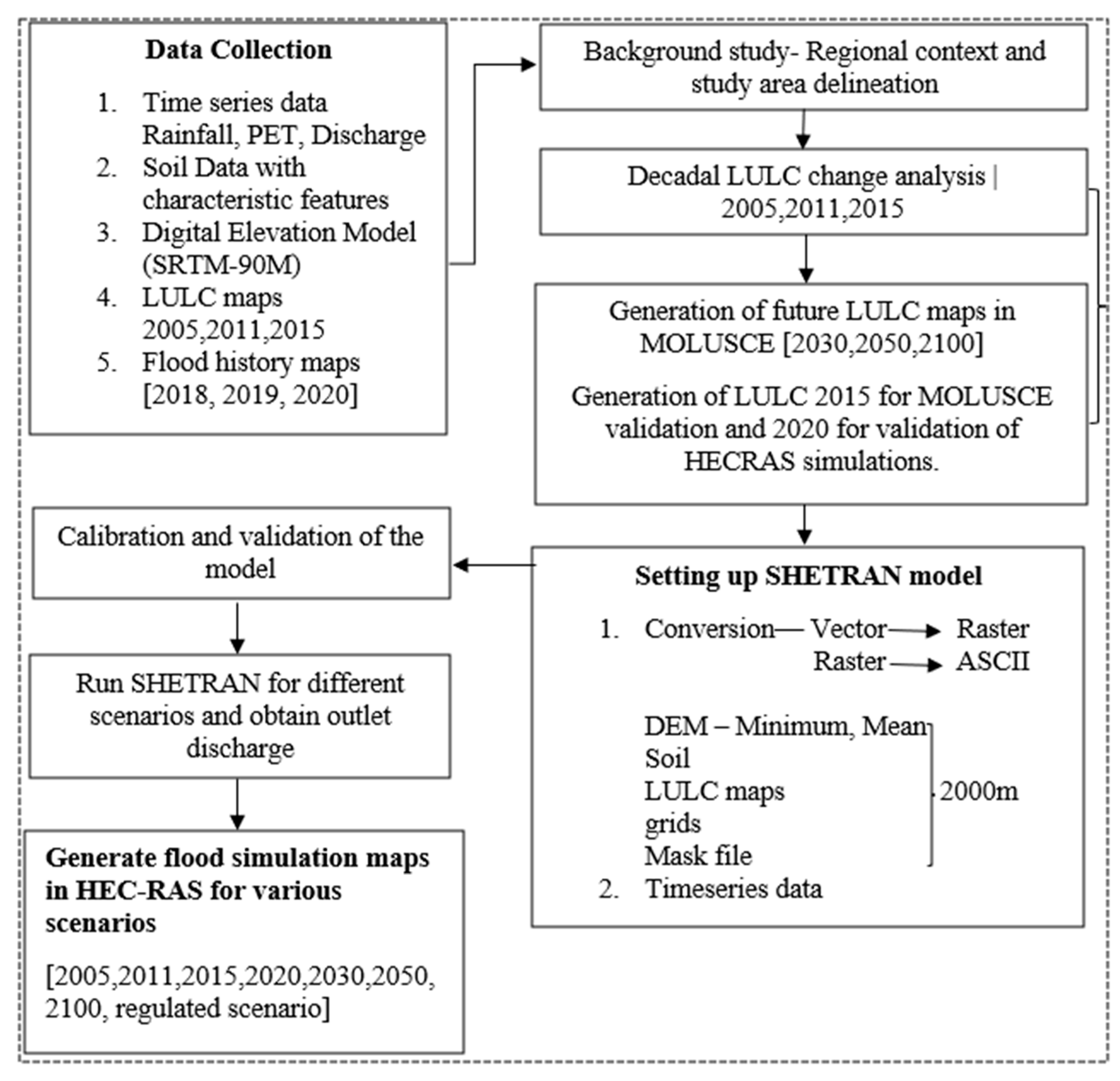
The NBS or regulated scenario considered two changes to the LULC maps with the aim of reducing flooding. Firstly, this was considered for the upper part of the catchment, where 21.3 km2 of mostly scrubland was converted to forest cover (Table 2 and Figure 4). This used the standard forest parameters. Secondly, in the floodplain by the conversion of 82.0 km2 to a wet meadow class where perennial grasses comprise more than 10 percent of the vegetation cover [64]. This was restored in order to increase the water holding capacity, allowing flood waters to spread over a larger region [16]. A very low value for the Strickler coefficient was used, increasing the roughness to reduce overland flow. The results of the SHETRAN simulation with the NBS LULC maps were fed through the HEC-RAS model and the results were compared to the LULC 2015 simulations.

2.7. Methodology

The overall methodology in the work can be seen in Figure 5. This started with data collection, then the analysis of the current LULC maps, the development of the future LULC maps, the hydrological simulation using SHETRAN, and the hydraulic simulation using HEC-RAS.

3. Results

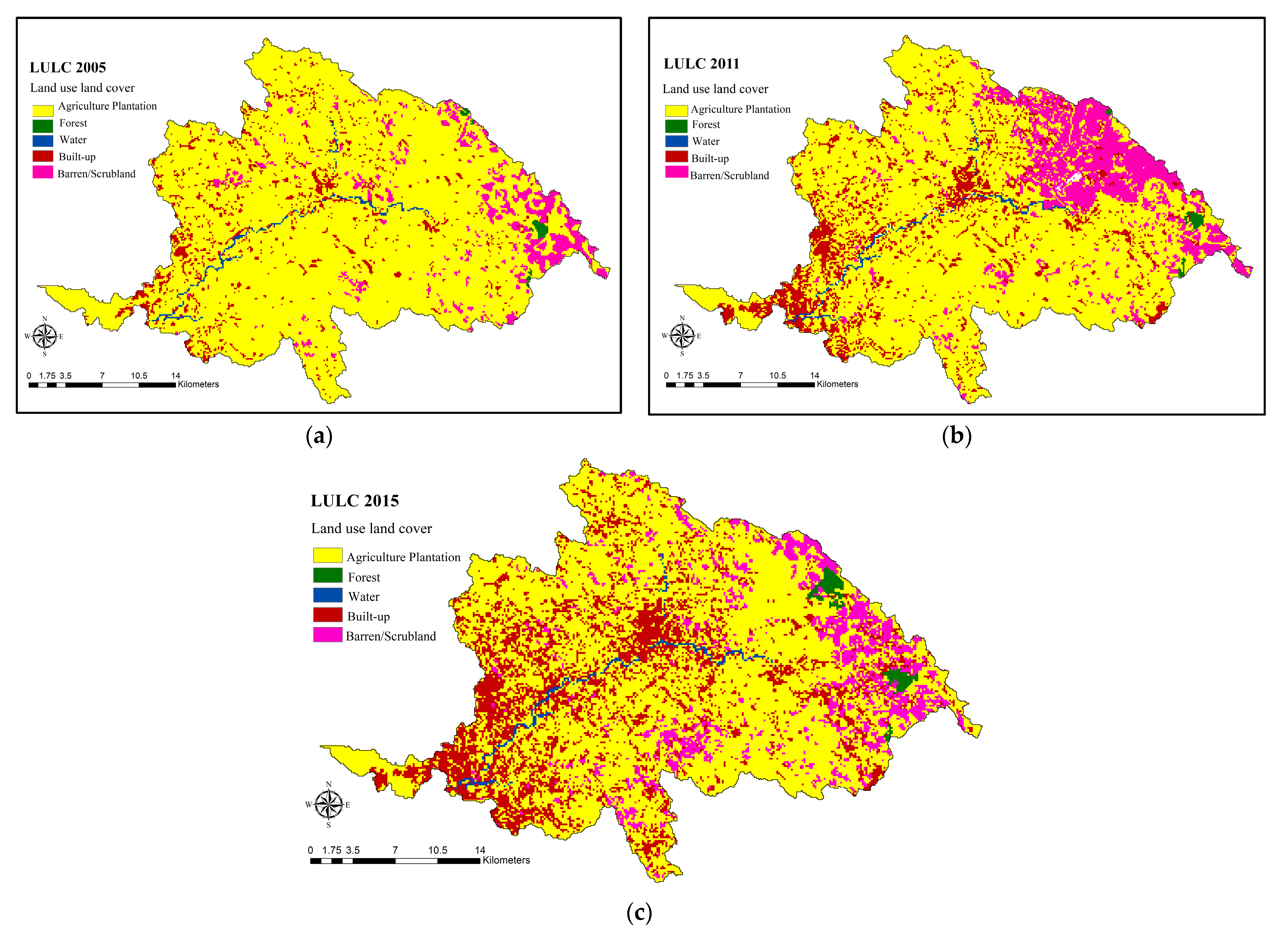
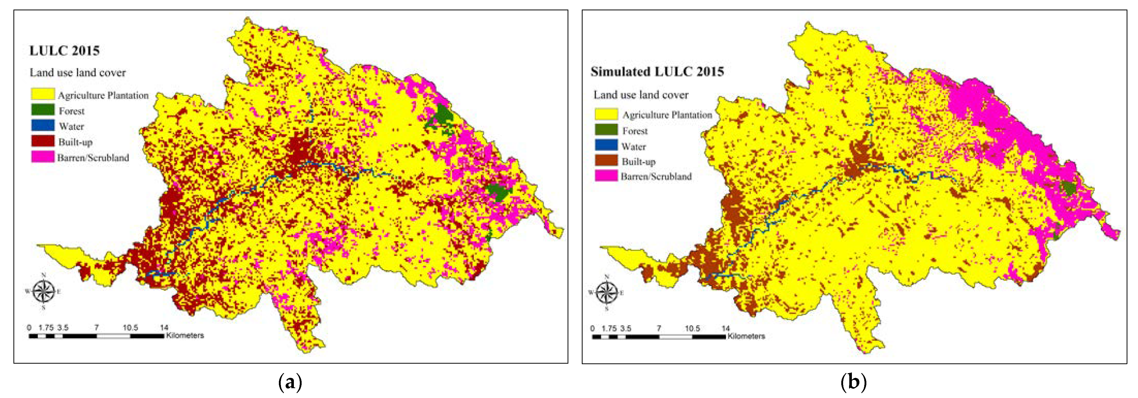
3.1. Validation of 2015 LULC Map and Future LULC Scenarios

The actual 2015 LULC map can be seen in Figure 6a together with the 2015 LULC map obtained from MOLUSCE (Figure 6b) based on the 2005 and 2011 maps. The comparison shows the percentage correctness is 90.9%. Both maps show an increase in the built-up area compared to 2005 and 2011 but the simulated LULC 2015 map shows too large an increase. This is considered to be acceptable but the consequence of this is considered in the Discussion (Section 4).
Figure 7a–c and Table 3 show the simulated future scenarios generated using MOLUSCE based on the historical LULC maps. The most significant change is the decrease in agricultural land from 567.1 km2 in 2015 to 463 km2 in 2100 and the corresponding increase in built-up/urban areas from 192.5 km2 in 2015 to 314.0 km2 in 2100. The future LULC maps show an overall Kappa statistic of 0.83 which is a reasonably good value, so validating the precision of the LULC maps generated.

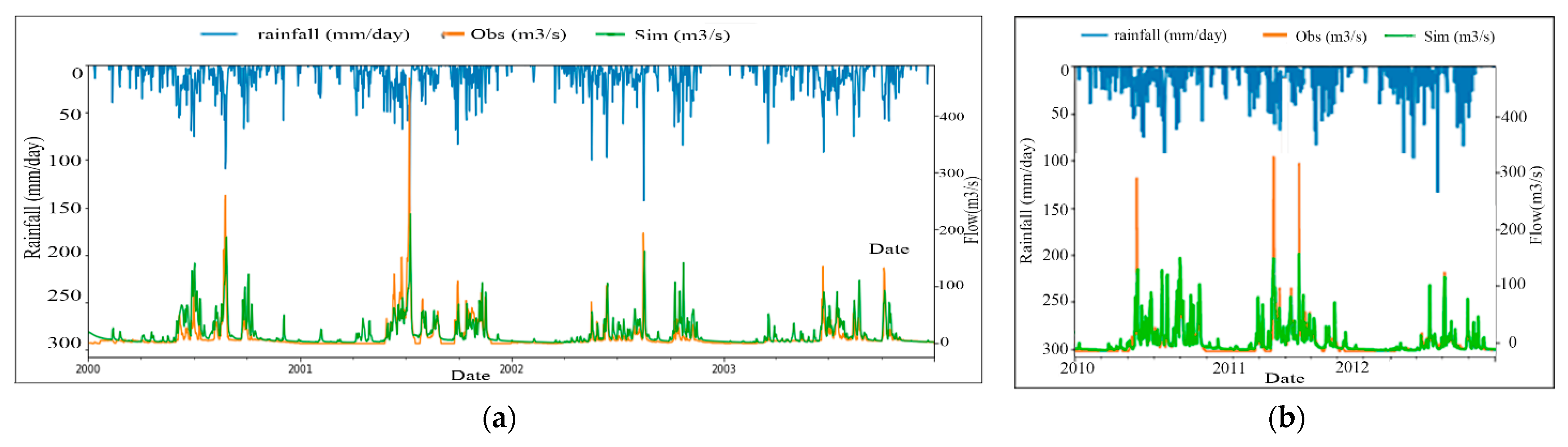
3.2. SHETRAN Calibration

The calibration runs are shown in the Appendix. The best calibration simulation produces an NSE of 0.63, PBIAS = 1.80, and KGE = 0.75 for daily discharges with the validation giving an NSE of 0.56, PBIAS = 5.60, and KGE = 0.72. The comparison between the measured and simulated discharge for four years in the calibration period and three years in the simulation period can be seen in Figure 8a,b. Overall, the quality of the simulations is considered to be fair to good [59,65]. The main issue with the simulation is having only two rain gauges over the entire 854 km2 catchment, which is insufficient to capture many of the highly localized convective rainfall events that occur in tropical regions [66]. This means some of the extreme rainfall events, such as in June 2001, which produced a peak discharge of 450 m3/s, are not captured by the simulation which has a peak value of 200 m3/s. Whereas, for other events, such as in October 2002 the simulated discharge is 150 m3/s, which is higher than the measured discharge of 50 m3/s. The other main issue in the simulations is that the discharges simulated during the dry season are too high, this can clearly be seen in the flow duration curves (Figure 9a,b). There may be some issues with the observed data here as the observed flows are often zero during these periods whereas the river is known to be perennial. As this work considers flooding, this issue will not significantly affect the results.

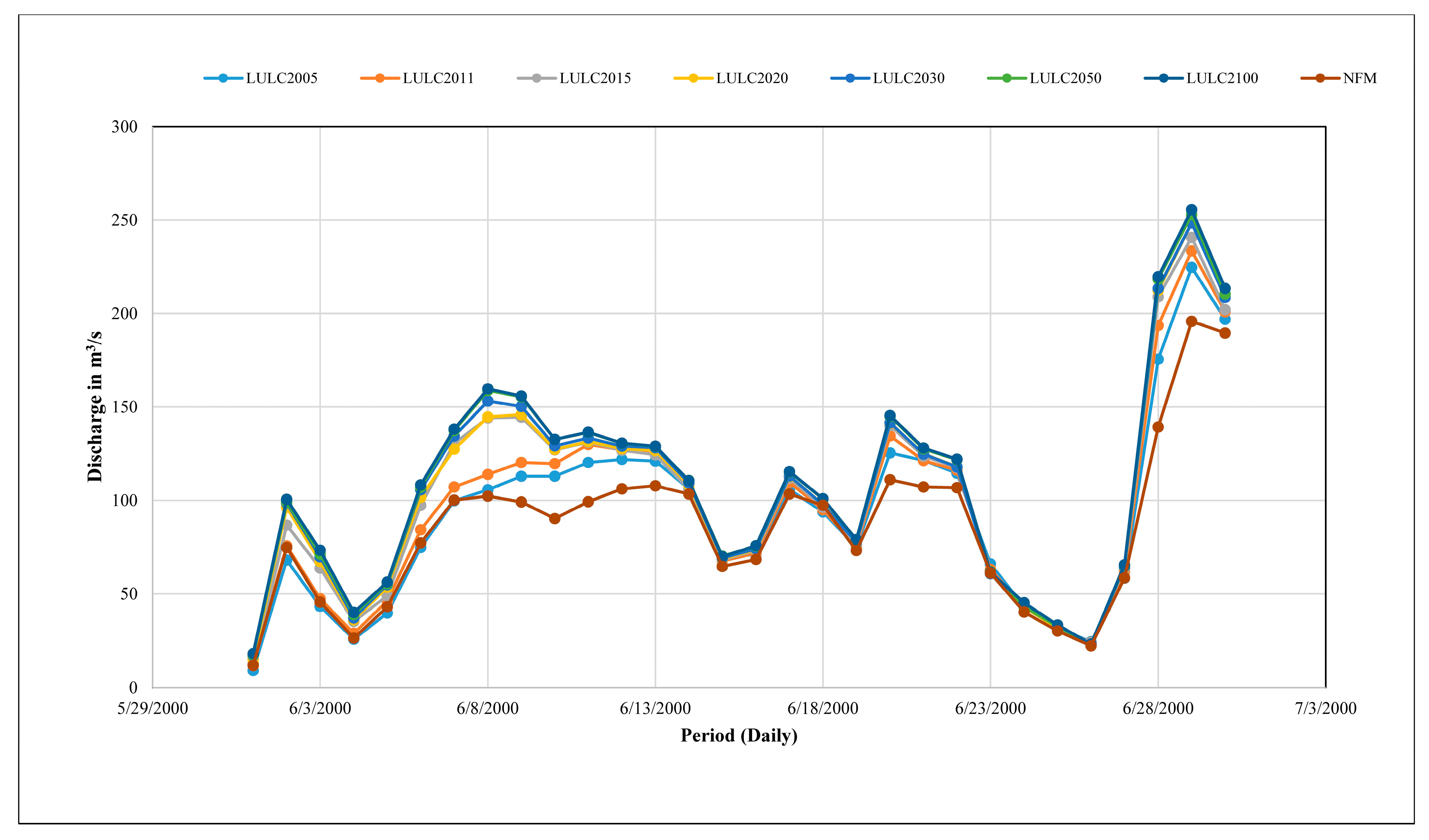
3.3. SHETRAN LULC Simulations

The simulated outlet discharge from the simulations for the seven different LULC simulations using rainfall and PET data for the period from June to November 2000 can be seen in Table 4. There is a clear pattern of increasing flow from 2005 to 2100 as the urban fraction within the catchment increases. Figure 10 considers the simulated discharges from June 2000 in detail. There is again a clear pattern of increasing discharge from 2005 to 2100 as the urban fraction increases. For instance, there is an increase of 8.5% in the average discharge in the month of August from 2005 to 2100. What is also clear is a higher absolute and relative difference in discharges for the larger discharges, such as for the rainfall event on 8 June 2000. Whereas, for low flow periods, such as on 26 June 2000, very similar flows are simulated for whichever LULC map is used. The bigger differences at high flows feed into the HEC-RAS model and produce a significant difference in the flooding downstream.
The SHETRAN results of using the NBS LULC map for the rainfall from June to November in 2020 can be seen in Table 4 and are compared with the discharge from the 2015 LULC; this shows a 13.1% reduction in flow. The results from June 2020 can also be seen in Figure 10, which shows the reduction is most significant for peak flows. This reduction is due to increased soil infiltration, higher soil and canopy evaporation and transpiration rates, and the increased storage of water, which is then gradually released [67].

3.4. HEC-RAS Simulations Validation

The validation of the HEC-RAS simulation map was carried out by a grid analysis approach, comparing the simulated flood map of 2020 against the observed flood map of 2020 (Figure 11). A grid resolution of 500 m × 500 m was adopted as the basis for analysis. A dot was assigned to every inundated cell in both cases (Figure 12) and the number of cells that exhibited flooding was quantified. The percentage of grids displaying inundation was subsequently calculated as a key metric for validating the concordance between the observed and simulated flood maps. It was found that there is an overall match of 81% which is reasonably good, with the simulated map overestimating the flooded area by 19%. The over-estimation could be for a number of reasons, including the accuracy of the inputs from the SHETRAN simulation, the resolution of the DEM used, and the accuracy of the observed flood map.

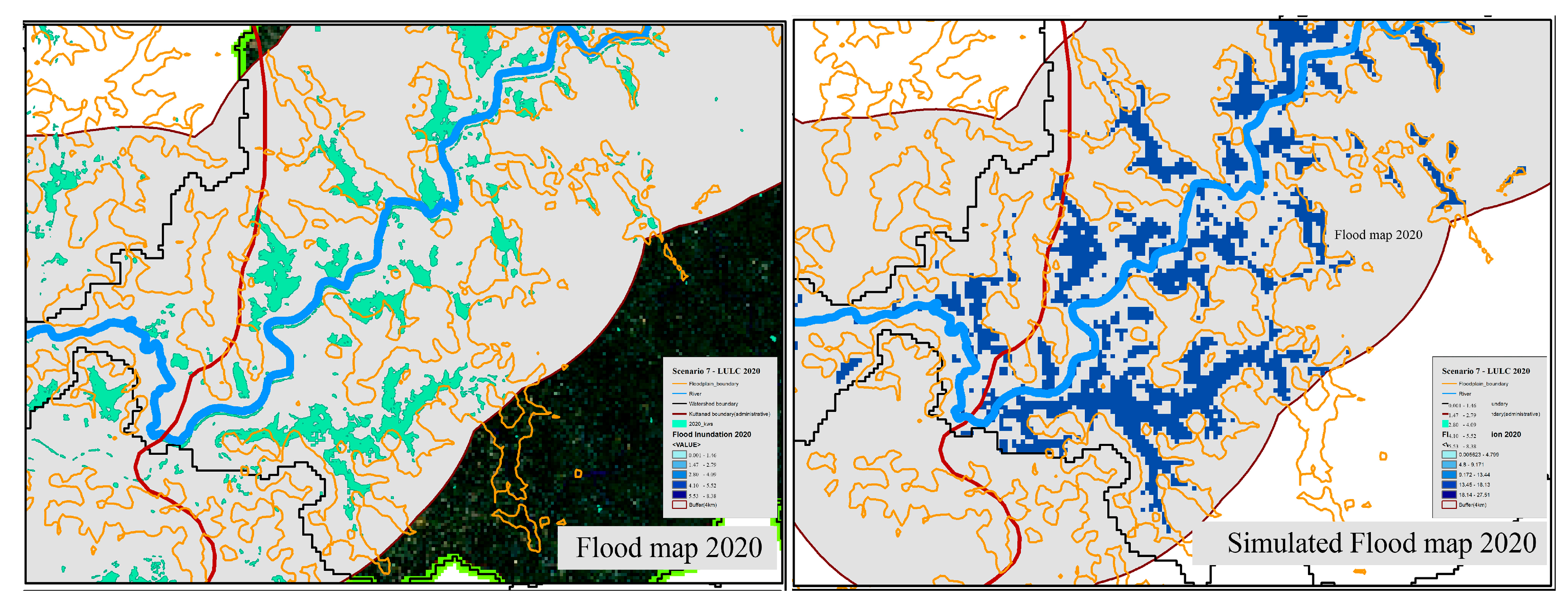
3.5. HEC-RAS LULC Scenario Simulations

Flood inundation maps were generated for each LULC scenario using HEC-RAS. The horizontal distribution of flood waters do not vary significantly between LULC scenarios. The difference caused by the changing LULC is predominantly reflected in the flood depth (Table 5). From 2005 to 2011, the average flood depth increases from 1.88 m to 2.94 m (83.1%) caused by a 6.5% increase in the urban area, an 8.3% increase in the barren area, and a 14.8% reduction in the agricultural area. Surprisingly, the flood depth has only grown by an additional 3.4% from 2011 to 2015, despite a further 9.9% increase in catchment built-up area. Beyond 2015, there is an increase in the urban area and a corresponding increase in the flood depth. By 2100, the average flood depth is 3.86 m compared to 1.88 m in 2005, a rise of 105%. For the NBS/regulated scenario, there is a reduction in flood depth from 3.04 m to 1.71 m (44%) compared to the LULC 2015 flood depth.

4. Discussion

4.1. Land Cover and NBS

The Meenachil river catchment and hence the KWS, which it flows into, are highly susceptible to flooding. The majority of the flooding occurs during the southwest monsoon (June–August), as there is often continuous rainfall for more than five days, allowing the soil to readily surpass its field capacity and get saturated, causing overland flow. Also, the issue is exacerbated by the steepness of the upstream region of the watershed (Figure 2c) and the fact that there is almost no native forest remaining in this part of the catchment (Figure 3). The results show that the increasing urbanization of the catchment is making the flooding worse, and this problem will only intensify in the future as more of the catchment is urbanized.
As well as urbanization, another issue regarding flooding is rubber plantations, which are classified as agriculture plantations in the LULC maps. The distribution of rubber across various gradients revealed that 49% was grown on slopes between 5 and 15%, which is optimal for its cultivation. The rest of the rubber plantations were on slopes with the potential for waterlogging, overland flow, and soil erosion issues [38]. Rubber cultivation cannot be taken over by an alternate crop as rubber has already become the livelihood of many people, both women and men, within the catchment. In order to ensure optimal development and output from rubber plantations, it is vital to implement necessary agricultural procedures in locations with land use change restrictions [38].
The increase in urbanization together with uncertainties brought on by a changing climate demand an increased emphasis on NBS, which has various co-benefits. However, developing a reproducible model is a precondition for identifying the potential role of NBS in reducing the frequency and severity of floods, so more research should be encouraged. According to this study, the rising impermeable ground cover upstream limits the infiltration capacity and leads to an increase in flow downstream, so drastically altering the catchment’s dynamics and morphology. The emphasis of restoration operations should be on indigenous tree and plant species that can resist extreme conditions and delay overland flow, enabling water to penetrate the aquifers and increase the baseflow upstream. As there are cases where reforestation has been shown to result in groundwater flooding [68], it is advised that the water table level be monitored continuously, and restoration operations continue slowly. The use of different flood risk control strategies is determined by the individual catchment characteristics, as there is no generalized way of approaching the catchment.

4.2. Planning Policy

Flooding in the KWS depends on the flows of the five river catchments that drain into the system. Figure 2 shows these catchments are in five districts within the state of Kerala, namely Ernakulam, Idukki, Kottayam, Alappuzha, and Pathanamthitta. Instead of commencing planning procedures with administrative divisions such as ward, panchayat (a village council), district, and state, the catchment boundary should be the new fundamental unit of planning. The new approach should have multiple layers including a flood risk assessment study, forecasts and implications of sea level rise and a changing climate, mapping of blue-green infrastructure, LULC change impact evaluations, water quality assessments, cost-benefit analyses, etc. [16,69]. It is absolutely necessary to have future predictions of events like floods, droughts, and other types of natural disasters; to determine high-risk zones that need to be given priority for protection; to set priorities and actions for stormwater management; to determine lands that can be developed; and to prioritize regions for infrastructure improvements and responsive action [16].
Emerging nations must adopt global best practices, such as the United Kingdom’s Catchment Flood Management Plans (CFMP) [70]. Integrating spatial planning and hydrology in the framework of a nation as a unified socio-ecological system is an outstanding endeavor that brings together all stakeholders.
In addition, it is crucial that the results of hydrological models be linked with the preparation of statutory plans. For instance, this study provided flood depth simulations with SHETRAN and HEC-RAS, which, when overlaid on the building map, can clearly predict which buildings are most likely to be submerged in water and the likely vertical rise in flood water. Thus, prompting an examination of various construction techniques resistant to the worst-case scenario. Based on economic considerations, the land management strategy should also determine if commercial, residential, or industrial buildings may give a higher degree of protection [71].
While the restoration of floodplains to their natural state and the initiation of relocation efforts are worth considering, they may raise complex issues related to property rights and land use [26,71]. Eventually, as the effects of urbanization and climate change increase flooding, relocating people from the floodplains might be a prerequisite, since investing in flood losses may not be sustainable in the long term. Due to familial obligations, livelihood prospects, financial limits, and emotional attachments, unassisted resettlement is not always a viable choice. Those who stay in a high risk area and those who leave may both display adaptability and resilience [24]. The policies of land swapping and the transfer of development rights (TDR) need consideration. Identifying government land for land swapping or land acquisition with financial support from the government may be a viable strategy, allowing individuals to maintain their current means of livelihood. Another important planning aspect is the effect of building patterns within built-up areas [72,73] with regulations that encourage vertical expansion having the potential to reduce urban flooding.
It was also obvious from the research that prohibiting the development of a set distance from rivers cannot be generalized since flooding in a location is determined by its elevation profile, whether it is low-lying or on higher ground. Therefore, a 50 or 100 m buffer from the creek [74] is insufficient for the intended goal. Similarly, it is crucial to increase the effectiveness of current construction codes regarding the necessary installation of rainwater harvesting systems (RHSs) for homes with a plinth area of more than 150 m2. Rather than a single visit during building approval after construction is complete, many inspections must be undertaken to confirm that the RHS is still in place since it is usual practice to remove the RHS after the building is sanctioned. This rule will secure the penetration of a certain amount of water at rainfall-receiving properties, as the average rainfall received is 3000 mm in the state of Kerala, therefore contributing to the elevation of the groundwater table by curtailing the stream flow downstream.
Likewise, it also becomes impertinent to develop a land use suitability map for agriculture practice by estimating the favorable climatic and soil conditions for various crops. Then, stringent restrictions can be imposed wherever it is inappropriate to practice them, depending on the gradient of the slope, the water retention capacity of the soil, and the canopy size of trees. The map should be made available to planners, bureaucrats, and farm owners to use it as a decision support tool [38].
An additional planning aspect is local or community-level engagement in developing planning recommendations. Research in India has shown that socially vulnerable people have lacked the ability to respond to floods [75,76]. So, developing the participation of these socially vulnerable local communities with urban planning to enable customized planning strategies is an important aspect that should be considered [77]. For example, the use of virtual reality enhances issues related to urban flooding, allowing laypersons to explore the expected impact of floods from various scenarios [77]. Working closely with the local people will provide insights into ground-level challenges and Indigenous knowledge which are impertinent to develop practical and informed decisions and place-based flood risk management strategies, also ensuring wider buy-in. In the same way, working closely with government bodies helps in integrating the research findings into existing policies and regulatory frameworks and converting them into actionable policies and development plans, while engaging the private sector such as businesses and developers can drive innovative solutions and investment in flood mitigation projects.
From this study, it could be summarized that spatial planning is seldom regarded as a flood mitigation tool, especially those addressing resilience to and rebound from flood risks [78]. This study proposes here several planning suggestions, which have the potential to be developed as an additional layer on top of this research.

4.3. Limitations

This study utilized a larger 2 km grid size (i.e., each grid square covers 2 km by 2 km) because smaller grid sizes required extensive computation time, which was not feasible given the time constraints. This study was carried out with the assumption that this grid size would provide reasonably good results with reference to the study by [79] that showed reasonably good results using 1 km, 2 km, and 4 km grid sizes and another study that utilized a coarse 5 km grid [80,81]. Similarly, this study was restricted to high-level methodology as a first step. Climate change has the potential to significantly affect future flooding and so further research is planned, incorporating climate change scenarios into the models.
There are other factors that contribute to predicting the future LULC maps not incorporated into the models, such as policy changes, population growth, migration, economic development, etc. These are potential deciding factors on how the future would look and how the actual vulnerability of the place is decided by socio-economic components, bio-physical components as well as the land use component. These factors could be introduced as additional layers in further studies. Due to time constraints and limited information access as well as the evolving nature of catchment-based planning, this study does not delve into how to overcome the challenges while transitioning from administrative-based conventional planning mechanisms. In addition, the data we utilized for this study were secondary data (online sources), as they were the best available data. Given the large scale of the study area and the lack of primary data to support specific interventions, this study had to be limited to general planning recommendations. However, these recommendations have the potential for further detailed exploration.

5. Conclusions

The KWS, Kerala, India has suffered significant flooding in recent years and the flooding seems to be becoming more frequent. In this work, recent LULC changes were analyzed and future LULC maps developed using MOLUSCE for the Meenachil river catchment, which is one of the five catchments draining into the KWS. These show a significant increase in urbanization in recent years, which is expected to continue due to the increasing population. Hydrological modeling using SHETRAN was carried out for the Meenachil river catchment with the calibration showing satisfactory results. Simulations were then run for the historic and future LULC maps and these show significant increases in total flows and peak flows as the catchment has urbanized between 2005 and 2015 and this trend is expected to continue under future land uses, and as such the total discharge from June to November 2020 is expected to be 11.2% higher for the 2100 LULC compared to the 2005 LULC. Flows from SHETRAN for the 2020 flooding event were then used as inputs for the detailed hydraulic model of the Meenachil river and its floodplain. Validation of the flooding extent against the measured data for 2020 shows a good correspondence. Results for a range of historic and future LULC maps for the same event then show an increase in flood depth as the catchment undergoes urbanization, with an expected increase from 1.88 m in 2005 to 3.86 m in 2100. This is expected to cause additional flooding in the KWS. These changes have been carried out using historic rainfall data, as when the temperature increases as the climate changes there is the potential for an intensified monsoon which will also increase the flooding potential in the KWS.
NBSs have the potential to help alleviate the flooding issues caused by the increasing urbanization. This was simulated by adding forest to the upland part of the catchment (2.5% of the catchment area), reverting some of the catchment back to its natural type. In addition, within the floodplain (9.6% of the catchment area), a wet meadow class was added, reducing the speed of flow. This had a significant effect on the flows, reducing the flooded depth by 44%. Although the effect on the flows was significant, there are a number of planning issues related to this which make it difficult to implement. The next layer on top of this research could be resolving the water governance for the system by integrating various plans and stakeholders into a single planning mechanism.
This study was primarily focused on the development of the methodology rather than the precision of the output, as there are issues with the quality of the data. The rainfall data and discharge data received from the State Irrigation Department of Kerala had data reliability issues. Further research could potentially use data from the Central Water Commission, who have installed a new station within the catchment, although the data are not publicly accessible. A finer resolution SHETRAN model could be applied which would help in exploring wider NFM techniques rather than restricting the simulations to regional scale interventions. This study considered only one of the five river basins draining into the KWS wetland system, and in future all the basins should be considered. Two of the river basins have reservoirs, and so they behave different hydrologically to the Meenachil river basin and would need reservoir operational data from the Kerala State Electricity Board.

Supplementary Materials

The following supporting information can be downloaded at: https://www.mdpi.com/article/10.3390/su16135652/s1, Table S1: Modified parameters for model sensitivity tests. AE/PE is the actual/potential evaporation rate at field capacity, SOC is the Strickler overland flow coefficient, K; Figure S1: Soil map of the river basin; Table S2: Soil characteristic features within the catchment.

Author Contributions

Conceptualization, S.T.S.; methodology, S.T.S.; software, S.T.S. and S.J.B.; validation, S.T.S. and S.J.B.; formal analysis, S.T.S.; investigation, S.T.S. and S.J.B.; resources, S.T.S. and S.J.B.; data curation, S.T.S. and S.J.B.; writing—original draft preparation, S.T.S.; writing—review and editing, S.T.S. and S.J.B.; visualization, S.T.S.; supervision, S.J.B.; project administration, S.T.S. and S.J.B.; funding acquisition, S.J.B. All authors have read and agreed to the published version of the manuscript.

Funding

This research received no external funding.

Institutional Review Board Statement

Not applicable.

Informed Consent Statement

Not applicable.

Data Availability Statement

Data are contained within the article and Supplementary Materials.

Acknowledgments

We are deeply grateful to Chris Kilsby for his invaluable mentorship and guidance during the corresponding author’s dissertation at Newcastle University, United Kingdom, which has significantly shaped this manuscript. We would also like to thank two anonymous reviewers for their insightful comments which have resulted in an improved manuscript.

Conflicts of Interest

Author Sonu Thaivalappil Sukumaran was employed by the company Arup. The remaining author declares that the research was conducted in the absence of any commercial or financial relationships that could be construed as a potential conflict of interest.

References

  1. Alshammari, E.; Rahman, A.A.; Rainis, R.; Seri, N.A.; Fuzi, N.F.A. The Impacts of Land Use Changes in Urban Hydrology, Runoff and Flooding: A Review. Curr. Urban Stud. 2023, 11, 120–141. [Google Scholar] [CrossRef]
  2. Dadashpoor, H.; Azizi, P.; Moghadasi, M. Land use change, urbanization, and change in land-scape pattern in a metropolitan area. Sci. Total Environ. 2019, 655, 707–719. [Google Scholar] [CrossRef]
  3. Barron, O.V.; Barr, A.D.; Donn, M.J. Effect of urbanisation on the water balance of a catchment with shallow groundwater. J. Hydrol. 2013, 485, 162–176. [Google Scholar]
  4. Sear, D.A.; Hornby, D.H.; Wheaton, J.; Hill, C.T. Understanding River Channel Sensitivity to Geomorphological Changes: Methods; Report FRS17183; Environment Agency: Bristol, UK, 2021. [Google Scholar]
  5. Verbeiren, B.; Van De Voorde, T.; Canters, F.; Binard, M.; Cornet, Y.; Batelaan, O. Assessing urbanisation effects on rainfall-runoff using a remote sensing supported modelling strategy. Int. J. Appl. Earth Obs. Geoinf. 2013, 21, 92–102. [Google Scholar] [CrossRef]
  6. Feng, B.; Zhang, Y.; Bourke, R. Urbanization impacts on flood risks based on urban growth data and coupled flood models. Nat. Hazards 2021, 106, 613–627. [Google Scholar] [CrossRef]
  7. Zope, P.E.; Eldho, T.I.; Jothiprakash, V. Impacts of urbanization on flooding of a coastal urban catchment: A case study of Mumbai City, India. Nat. Hazards 2015, 75, 887–908. [Google Scholar] [CrossRef]
  8. Sadashivam, T.; Tabassu, S. Trends of urbanization in India: Issues and challenges in the 21st century. Int. J. Inf. Res. Rev. 2016, 3, 2375–2384. [Google Scholar]
  9. Lal, P.; Nair, S.B. Urbanization in Kerala—What does the census data reveal? Indian J. Hum. Dev. 2017, 11, 356–386. [Google Scholar]
  10. Gosling, S.N.; Lewis, E.; Birkinshaw, S.J.; Tratalos, J.; Haines-Young, R. The Effects of Future Land-Cover Change on UK River Flows. Available online: https://citeseerx.ist.psu.edu/document?repid=rep1&type=pdf&doi=073527e0ef77dc6aa88667a113f6dce694ecf61b (accessed on 15 June 2024).
  11. Mekonnen, D.; Duan, Z.; Rientjes, T.; Disse, M. Analysis of the combined and single effects of LULC and climate change on the streamflow of the Upper Blue Nile River Basin (UBNRB): Using statistical trend tests, remote sensing landcover maps and the SWAT model. Hydrol. Earth Syst. Sci. Discuss. 2017, 1–26. [Google Scholar]
  12. Yereseme, A.K.; Surendra, H.J.; Kuntoji, G. Sustainable integrated urban flood management strategies for planning of smart cities: A review. Sustain. Water Resour. Manag. 2022, 8, 85. [Google Scholar] [CrossRef]
  13. Zhou, Q.; Leng, G.; Su, J.; Ren, Y. Comparison of urbanization and climate change impacts on urban flood volumes: Importance of urban planning and drainage adaptation. Sci. Total Environ. 2019, 658, 24–33. [Google Scholar] [CrossRef] [PubMed]
  14. Arnold, J.G.; Srinivasan, R.; Muttiah, R.S.; Williams, J.R. Large area hydrologic modeling and assessment part I: Model development. J. Am. Water Resour. Assoc. 1998, 34, 73–89. [Google Scholar] [CrossRef]
  15. Bathurst, J.C.; Ewen, J.; Parkin, G.; O’Connell, P.E.; Cooper, J.D. Validation of catchment models for predicting land-use and climate change impacts. 3. Blind validation for internal and outlet responses. J. Hydrol. 2004, 287, 74–94. [Google Scholar] [CrossRef]
  16. Sonu, T.S.; Bhagyanathan, A. The impact of upstream land use land cover change on downstream flooding: A case of Kuttanad and Meenachil River Basin, Kerala, India. Urban Clim. 2022, 41, 101089. [Google Scholar]
  17. Munoth, P.; Goyal, R. Impacts of land use land cover change on runoff and sediment yield of Upper Tapi River Sub-Basin, India. Int. J. River Basin Manag. 2020, 18, 177–189. [Google Scholar] [CrossRef]
  18. Abe, C.A.; Lobo, F.D.L.; Dibike, Y.B.; Costa, M.P.D.F.; Dos Santos, V.; Novo, E.M.L. Modelling the effects of historical and future land cover changes on the hydrology of an Amazonian basin. Water 2018, 10, 932. [Google Scholar] [CrossRef]
  19. Chu, M.L.; Knouft, J.H.; Ghulam, A.; Guzman, J.A.; Pan, Z. Impacts of urbanization on river flow frequency: A controlled experimental modeling-based evaluation approach. J. Hydrol. 2013, 495, 1–12. [Google Scholar] [CrossRef]
  20. De Hipt, F.O.; Diekkrüger, B.; Steup, G.; Yira, Y.; Hoffmann, T.; Rode, M. Modeling the effect of land use and climate change on water resources and soil erosion in a tropical West African catchment (Dano, Burkina Faso) using SHETRAN. Sci. Total Environ. 2019, 653, 431–445. [Google Scholar] [CrossRef]
  21. Sreedevi, S.; Eldho, T.I.; Jayasankar, T. Physically based distributed modelling of the hydrology and soil erosion under changes in landuse and climate of a humid tropical river basin. Catena 2022, 217, 106427. [Google Scholar] [CrossRef]
  22. Song, X.; Zhang, J.; Zhan, C.; Xuan, Y.; Ye, M.; Xu, C. Global sensitivity analysis in hydrological modeling: Review of concepts, methods, theoretical framework, and applications. J. Hydrol. 2015, 523, 739–757. [Google Scholar] [CrossRef]
  23. Alahmad, S.; Bin Abdullah, R.; Abustan, I.; Eslamian, S. Comparison between capabilities of HEC-RAS and MIKE11 hydraulic models in river flood risk modeling (A case study of Sungai Kayu Ara River basin, Malaysia). Int. J. Hydrol. Sci. Technol. 2012, 2, 270–291. [Google Scholar]
  24. Hadimlioglu, I.A.; King, S.A.; Starek, M.J. FloodSim: Flood simulation and visualization framework using position-based fluids. ISPRS Int. J. Geo-Inf. 2020, 9, 163. [Google Scholar] [CrossRef]
  25. India, L. Lakes of India Kuttanad: The Rice Bowl of Kerala. InfoSWMM Help Documentation. 2022, pp. 8–12. Available online: https://help.innovyze.com/space/infoswmm/17598253/Introduction (accessed on 15 June 2024).
  26. Hartmann, T.; Juepner, R. The Flood Risk Management Plan: An Essential Step Towards the Institutionalization of a Paradigm Shift. Int. J. Water Gov. 2014, 2, 107–118. [Google Scholar] [CrossRef]
  27. Pathak, S.; Liu, M.; Jato-Espino, D.; Zevenbergen, C. Social, economic and environmental assessment of urban sub-catchment flood risks using a multi-criteria approach: A case study in Mumbai City, India. J. Hydrol. 2020, 591, 125216. [Google Scholar] [CrossRef]
  28. Sowińska-Świerkosz, B.; García, J. What is Nature-based solutions (NBS)? Setting core ideas for concept clarification. Nat. Based Solut. 2022, 2, 100009. [Google Scholar] [CrossRef]
  29. Faivre, N.; Fritz, M.; Freitas, T.; de Boissezon, B.; Vandewoestijne, S. Nature-Based Solutions in the EU: Innovating with nature to address social, economic and environmental challenges. Environ. Res. 2017, 159, 509–518. [Google Scholar] [CrossRef]
  30. Sreeja, K.G.; Madhusoodhanan, C.G.; Eldho, T.I. Climate and Landuse Change Impacts on Sub-Sea Level Rice Farming in a Tropical Deltaic Wetland. In Proceedings of the 36th IAHR World Congress, The Hague, The Netherlands, 28 June–3 July 2015; pp. 1–8. [Google Scholar]
  31. Gopakumar, M. Kuttanad: The Next Vanishing Wetland? 2022. Available online: https://frontline.thehindu.com/environment/will-kuttanad-be-the-next-vanishing-wetland/article65546163.ece (accessed on 21 August 2022).
  32. Varughese, A. Climate Change Has Cost Kuttanad Farmers Rs 9, 608 Crore This Year. Here’ s What Can Help. 2022. Available online: https://thewire.in/agriculture/kerala-kuttanad-farmers-rainfall-paddy (accessed on 5 April 2022).
  33. Biju, E.P. Kainakari in Kerala’ s Kuttanad in knee-deep water for past 78 days. September 2018. pp. 1–3. Available online: https://www.newindianexpress.com/states/kerala/2018/Sep/01/kainakari-in-keralas-kuttanad-in-knee-deep-water-for-past-78-days-1866181.html#:~:text=The%20sexagenarian%20farmer%20has%20been,%2C%20and%20son%20Biju%2C%2038 (accessed on 5 April 2022).
  34. Shaji, K. In Kerala’s Kuttanad, Climate Change Is Forcing Locals to Abandon Their Homes. 2021, pp. 1–11. Available online: https://scroll.in/article/1003721/in-keralas-kuttanad-climate-change-is-forcing-residents-to-abandon-their-homes (accessed on 21 August 2022).
  35. Kumar, B.A.; Gopinath, G.; Chandran, M.S. River sinuosity in a humid tropical river basin, southwest coast of India. Arab. J. Geosci. 2014, 7, 1763–1772. [Google Scholar] [CrossRef]
  36. NRSC. Bhuvan|ISRO’s Geoportal|Gateway to Indian Earth Observation. Available online: https://www.nrsc.gov.in/ (accessed on 15 June 2024).
  37. Vinayak, A.J. Borewells depleting water of future generations: Experts. 2018. Available online: https://www.thehindubusinessline.com/news/borewells-depleting-water-of-future-generations-experts/article64332492.ece (accessed on 21 August 2022).
  38. Meti, S.; Rao, D.V.K.N.; Nair, N.U.; Jacob, J. Distribution of natural rubber cultivation in relation to soil and landscape attributes in India. In Proceedings of the 29th Asian Conference on Remote Sensing 2008, ACRS 2008, Colombo, Sri Lanka, 10–14 November 2008; pp. 7–16. [Google Scholar]
  39. Sethunath, K. Rubber Economy in Crisis. 2016, pp. 1–8. Available online: https://www.deccanchronicle.com/nation/current-affairs/100216/rubber-economy-in-crisis.html (accessed on 22 May 2022).
  40. Onmanorama. Post Floods Slender Meenachil River Raises Concern. 2018. Available online: https://www.onmanorama.com/lifestyle/news/2018/09/01/post-floods-slender-meenachil-river-raises-concern.html (accessed on 22 May 2022).
  41. Chughtai, A.H.; Abbasi, H.; Karas, I.R. A review on change detection method and accuracy assessment for land use land cover. Remote Sens. Appl. Soc. Environ. 2021, 22, 100482. [Google Scholar] [CrossRef]
  42. Xu, S.; Sheng, G.; Boyd, S.A. Use of Organoclays in Pollution Abatement. Adv. Agron. 1997, 59, 25–62. [Google Scholar]
  43. Zomer, R.J.; Xu, J.; Trabucco, A. Version 3 of the global aridity index and potential evapotranspiration database. Sci. Data 2022, 9, 409. [Google Scholar] [CrossRef] [PubMed]
  44. Woodroffe, C.D.; Falkland, A.C. Chapter 31 Geology and hydrogeology of the Cocos (Keeling) islands. Dev. Sedimentol. 2004, 54, 885–908. [Google Scholar]
  45. Rahman, M.T.U.; Tabassum, F.; Rasheduzzaman, M.; Saba, H.; Sarkar, L.; Ferdous, J.; Uddin, S.Z.; Zahedul Islam, A.Z.M. Temporal dynamics of land use/land cover change and its prediction using CA-ANN model for southwestern coastal Bangladesh. Environ. Monit. Assess. 2017, 189, 29039035. [Google Scholar] [CrossRef]
  46. Guzha, A.C.; Rufino, M.C.; Okoth, S.; Jacobs, S.; Nóbrega, R.L.B. Impacts of land use and land cover change on surface runoff, discharge and low flows: Evidence from East Africa. J. Hydrol. Reg. Stud. 2018, 15, 49–67. [Google Scholar] [CrossRef]
  47. Mubea, K.W.; Ngigi, T.G.; Mundia, C.N. Assessing Application of Markov Chain Analysis in Nakuru. J. Agric. Sci. Technol. 2011, 12, 126. [Google Scholar]
  48. Maxwell, A.E.; Warner, T.A.; Fang, F. Implementation of machine-learning classification in remote sensing: An applied review. Int. J. Remote Sens. 2018, 39, 2784–2817. [Google Scholar] [CrossRef]
  49. Ngoy, K.I.; Qi, F.; Shebitz, D.J. Analyzing and Predicting Land Use and Land Cover Changes in New Jersey Using Multi-Layer Perceptron–Markov Chain Model. Earth 2021, 2, 845–870. [Google Scholar] [CrossRef]
  50. Hasan, S.; Shi, W.; Zhu, X.; Abbas, S.; Khan, H.U.A. Future simulation of land use changes in rapidly urbanizing South China based on land change modeler and remote sensing data. Sustainability 2020, 12, 4–6. [Google Scholar] [CrossRef]
  51. Leta, M.K.; Demissie, T.A.; Tränckner, J. Modeling and prediction of land use land cover change dynamics based on land change modeler (Lcm) in nashe watershed, upper blue nile basin, Ethiopia. Sustainability 2021, 13, 3740. [Google Scholar] [CrossRef]
  52. Kamaraj, M.; Rangarajan, S. Predicting the future land use and land cover changes for Bhavani basin, Tamil Nadu, India, using QGIS MOLUSCE plugin. Environ. Sci. Pollut. Res. 2022, 29, 86337–86348. [Google Scholar] [CrossRef]
  53. Isinkaralar, O. QGIS-based modeling and analysis of urban dynamics affecting land surface temperature towards climate hazards in coastal zones of Portugal. Nat. Hazards 2024, 120, 7749–7764. [Google Scholar] [CrossRef]
  54. Kafy, A.A.; Al Rakib, A.; Roy, S.; Ferdousi, J.; Raikwar, V.; Kona, M.A.; Al Fatin, S.A. Predicting changes in land use/land cover and seasonal land surface temperature using multi-temporal landsat images in the northwest region of Bangladesh. Heliyon 2021, 7, e07623. [Google Scholar] [CrossRef]
  55. Elmahdy, S.I.; Mohamed, M.M. Remote sensing and geophysical survey applications for delineating near-surface palaeochannels and shallow aquifer in the United Arab Emirates. Geocarto Int. 2015, 30, 723–736. [Google Scholar] [CrossRef]
  56. Arumugam, T. Assessment and Predicting of LULC by Kappa Analysis and CA Markov model using RS and GIS Techniques in Udham Singh Nagar District, India. Res. Square 2021, 3. [Google Scholar] [CrossRef]
  57. Ewen, J.; Parkin, G.; O’Connell, P.E. SHETRAN: Distributed River Basin Flow and Transport Modeling System. J. Hydrol. Eng. 2000, 5, 250–258. [Google Scholar] [CrossRef]
  58. Anderton, S.P.; Latron, J.; White, S.M.; Llorens, P.; Gallart, F.; Salvany, C.; O’Connell, P.E. Internal evaluation of a physically based distributed model using data from a Mediterranean mountain catchment. Hydrol. Earth Syst. Sci. 2002, 6, 67–83. [Google Scholar] [CrossRef]
  59. Moriasi, D.N.; Gitau, M.W.; Pai, N.; Daggupati, P. Hydrologic and water quality models: Performance measures and evaluation criteria. Trans. ASABE (Am. Soc. Agric. Biol. Eng.) 2015, 58, 1763–1785. [Google Scholar]
  60. Liu, D. A rational performance criterion for hydrological model. J. Hydrol. 2020, 590, 1–23. [Google Scholar] [CrossRef]
  61. Lewis, E.; Birkinshaw, S.; Kilsby, C.; Fowler, H.J. Development of a system for automated setup of a physically based, spatially distributed hydrological model for catchments in Great Britain. Environ. Model. Softw. 2018, 108, 102–110. [Google Scholar] [CrossRef]
  62. Sreedevi, S.; Eldho, T.I.; Madhusoodhanan, C.G.; Jayasankar, T. Multiobjective sensitivity analysis and model parameterization approach for coupled streamflow and groundwater table depth simulations using SHETRAN in a wet humid tropical catchment. J. Hydrol. 2019, 579, 124217. [Google Scholar] [CrossRef]
  63. Krest Engineers. Manning’ s n (Roughness Coefficient) for HEC-RAS 2D Modeling. 2021. Available online: https://rashms.com/blog/mannings-n-roughness-coefficient-for-hec-ras-2d-modeling/ (accessed on 2 July 2022).
  64. Dieck, J.; Ruhser, J.; Hoy, E.; Robinson, L. General Classification Handbook for Floodplain Vegetation in Large River Systems; U.S. Geological Survey Techniques and Methods 2; U.S. Geological Survey: Reston, VA, USA, 2015; pp. 1–51. [Google Scholar]
  65. Cardoso de Salis, H.H.; Monteiro da Costa, A.; Moreira Vianna, J.H.; Azeneth Schuler, M.; Künne, A.; Sanches Fernandes, L.F.; Leal Pacheco, F.A. Hydrologic modeling for sustainable water resources management in urbanized karst areas. Int. J. Environ. Res. Public Health 2019, 16, 2542. [Google Scholar] [CrossRef]
  66. Suroso, S.; Santoso, P.B.; Birkinshaw, S.; Kilsby, C.; Bardossy, A.; Aldrian, E. Assessment of TRMM rainfall data for flood modelling in three contrasting catchments in Java, Indonesia. J. Hydroinform. 2023, 25, 797–814. [Google Scholar] [CrossRef]
  67. Buechel, M.; Slater, L.; Dadson, S. Hydrological impact of widespread afforestation in Great Britain using a large ensemble of modelled scenarios. Commun. Earth Environ. 2022, 3, 6. [Google Scholar] [CrossRef]
  68. Allen, A.; Chapman, D. Impacts of afforestation on groundwater resources and quality. Hydrogeol. J. 2001, 9, 390–400. [Google Scholar] [CrossRef]
  69. Anonymous. Watershed-Based Planning. Available online: https://wetlandswatch.org/watershed-based-planning/ (accessed on 29 May 2022).
  70. Falconer, R.A.; Harpin, R. Catchment flood management: A UK perspective and experience. Water Int. 2005, 30, 5–13. [Google Scholar] [CrossRef]
  71. Thomas, N.W.; Amado, A.A.; Schilling, K.E.; Weber, L.J. Evaluating the efficacy of distributed detention structures to reduce downstream flooding under variable rainfall, antecedent soil, and structural storage conditions. Adv. Water Resour. 2016, 96, 74–87. [Google Scholar] [CrossRef]
  72. Li, Z.; Wang, Z.; Wu, L.; Huang, W.; Peng, W. Evaluating the effect of building patterns on urban flooding based on a boosted regression tree: A case study of Beijing, China. Hydrol. Process. 2023, 37, e14932. [Google Scholar] [CrossRef]
  73. Huang, Y.; Lin, J.; He, X.; Lin, Z.; Wu, Z.; Zhang, X. Assessing the scale effect of urban vertical patterns on urban waterlogging: An empirical study in Shenzhen. Environ. Impact Assess. Rev. 2024, 106, 107486. [Google Scholar] [CrossRef]
  74. Ramachandran, A.; Enserink, B.; Balchand, A.N. Coastal regulation zone rules in coastal panchayats (villages) of Kerala, India vis-à-vis socio-economic impacts from the recently introduced peoples’ participatory program for local self-governance and sustainable development. Ocean Coast Manag. 2005, 48, 632–653. [Google Scholar] [CrossRef]
  75. Sam, A.S.; Kumar, R.; Kächele, H.; Müller, K. Vulnerabilities to flood hazards among rural households in India. Nat. Hazards 2017, 88, 1133–1153. [Google Scholar] [CrossRef]
  76. Das, S.; Hazra, S.; Haque, A.; Rahman, M.; Nicholls, R.J.; Ghosh, A.; Ghosh, T.; Salehin, M.; De Campos, R.S. Social vulnerability to environmental hazards in the Ganges-Brahmaputra-Meghna delta, India and Bangladesh. Int. J. Disaster Risk Reduct. 2021, 53, 101983. [Google Scholar] [CrossRef]
  77. Park, S.; Kim, J.; Kim, Y.; Kang, J. Participatory Framework for Urban Pluvial Flood Modeling in the Digital Twin Era. Sustain. Cities Soc. 2024, 108, 105496. [Google Scholar] [CrossRef]
  78. Ran, J.; Nedovic-Budic, Z. Integrating spatial planning and flood risk management: A new conceptual framework for the spatially integrated policy infrastructure. Comput. Environ. Urban Syst. 2016, 5768–5779. [Google Scholar] [CrossRef]
  79. Sreedevi, S.; Eldho, T.I. Effects of grid-size on effective parameters and model performance of SHETRAN for estimation of streamflow and sediment yield. Int. J. River Basin Manag. 2021, 19, 535–551. [Google Scholar] [CrossRef]
  80. Oliveira, A.R.; Ramos, T.B.; Simionesei, L.; Gonçalves, M.C.; Neves, R. Modeling Streamflow at the Iberian Peninsula Scale Using MOHID-Land: Challenges from a Coarse Scale Approach. Water 2022, 14, 1013. [Google Scholar] [CrossRef]
  81. Op de Hipt, F.; Diekkrüger, B.; Steup, G.; Yira, Y.; Hoffmann, T.; Rode, M. Applying SHETRAN in a tropical west African catchment (Dano, Burkina Faso)—Calibration, validation, uncertainty assessment. Water 2017, 9, 101. [Google Scholar] [CrossRef]
Figure 1. Geographical and administrative boundaries related to the Kuttanad Wetland System: (a) the Kuttanad administrative area and the five main river catchments that flow into the Kuttanad Wetland System (Source: Sonu, T.S., 2022 [16]); (b) the Kuttanad administrative boundary with the district boundaries and the Meenachil catchment boundary.
Sustainability 16 05652 g001
Figure 2. Hydrological characteristics of the Meenachil River Basin: (a) The catchment boundary of the Meenachil river basin and how it adjoins the Kuttanad administrative area with the rain gauge stations and discharge station within the basin; (b) sectional elevation of the watershed from Google Earth; and (c) river network with the degree of slope of the basin area.
Sustainability 16 05652 g002
Figure 3. Land use and land cover changes over time: (a) LULC map for 2005; (b) LULC map for 2011; and (c) LULC map for 2015.
Sustainability 16 05652 g003
Figure 4. NBS LULC map.
Sustainability 16 05652 g004
Figure 5. Methodology of the research.
Sustainability 16 05652 g005
Figure 6. Comparison of LULC maps for 2015: (a) reference LULC map 2015; (b) simulated LULC map 2015 using MOLUSCE.
Sustainability 16 05652 g006
Figure 7. Projected LULC changes: (a) simulated LULC map for 2030; (b) simulated LULC map for 2050; and (c) simulated LULC map for 2100.
Sustainability 16 05652 g007
Figure 8. Comparison of observed and simulated flow with rainfall data: (a) rainfall, observed, and simulated flow for part of the calibration period, 2000–2003, (b) observed and simulated flow for part of the validation period, 2010–2012.
Sustainability 16 05652 g008
Figure 9. Flow duration curves for calibration and validation periods: (a) flow duration curve for the calibration period (2000–2007); (b) flow duration curve comparison for the validation period (2008–2015).
Sustainability 16 05652 g009
Figure 10. Mean daily discharges for the 8 different LULC maps (the seven standard scenarios and the NBS scenario).
Sustainability 16 05652 g010
Figure 11. Validation of the HEC-RAS simulated flood inundation map against the reference flood history map of 2020. This shows the main river channel and the simulated 4 km buffer.
Sustainability 16 05652 g011
Figure 12. Grid analysis of the 2020 flooding event: (a) observed and (b) simulated grid analysis for the 2020 flooding event. The dots show cells that exhibit flooding. The highlighted area shows the approximate location where the observed and simulated events are most different.
Sustainability 16 05652 g012
Table 1. LULC areas (km2) and the changes from 2005.
Land Use2005 (km2)2011
(km2)
Difference (km2)Difference (%)2015 (km2)Difference (km2)Difference (%)
Agriculture739.9613.4−126.5−17.09567.1−172.8−23.35
Forest2.72.80.13.78.25.5203.7
Water6.46.60.23.17.00.69.4
Built-up/
urban
53.1108.455.3104.1192.5139.4262.5
Barren51.9122.870.9136.679.227.352.6
Table 2. Percentage LULC change (2015 vs. regulated scenario).
Land Use2015 (km2)Regulated
(km2)
Difference (km2)Difference (%)
Agriculture567.1486.5−80.6−14.2
Forest8.28.20.0
Water7.07.00.0
Built-up192.5185.0−7.5−3.8
Barren/Scrubland79.264.0−15.2−19.0
NBS (Flood Plain)-82.082.0-
NBS (Afforestation)-21.321.3-
Table 3. Future LULC maps generated using MOLUSCE.
Land Use 2015
(km2)
2030
(km2)
2050
(km2)
2100
(km2)
Difference
2015–2100 (km2)
Agriculture567.1497.2478.8463.0−102.1
Forest8.20.20.20.2−8.0
Water7.01.31.31.3−5.7
Built-up/Urban192.5278.4297.8314.0121.5
Barren79.276.975.975.5−3.7
Table 4. Mean outlet discharge simulated in SHETRAN (m3/s).
LULC2005201120152020203020502100NFM
Southwest Monsoon:
June91.896.2102.1103.9105.5107.5108.485.3
July79.981.983.984.985.486.086.975.6
August138.5143.0146.5148.5149.2150.6151.3122.7
Northeast Monsoon:
October45.446.847.748.048.549.049.642.8
November10.610.811.211.211.311.411.510.3
Table 5. Scenario-based flood depth and its correlation with land use (only the main land uses are shown so the percentages do not add up to 100).
ScenarioAgriculture (%)Built-Up/
Urban
(%)
Barren (%)NFM Forest/
Regulated (%)
Flood
Depth (m)
200586.66.26.0-1.88
201171.812.714.3-2.94
201566.422.69.3-3.04
203058.132.69.0-3.80
205056.034.98.9-3.84
210054.234.88.9-3.86
Regulated56.9621.67.4912.11.71
Disclaimer/Publisher’s Note: The statements, opinions and data contained in all publications are solely those of the individual author(s) and contributor(s) and not of MDPI and/or the editor(s). MDPI and/or the editor(s) disclaim responsibility for any injury to people or property resulting from any ideas, methods, instructions or products referred to in the content.

