


Estimating the Temporal Impacts of Nearshore Fisheries on Coastal Ocean-Sourced Waste Accumulation in South Korea Using Stepwise Regression

 ,
, 

Abstract
:1. Introduction
2. Materials and Methods
2.1. Data Collection
2.1.1. Coastal Waste Monitoring Data
2.1.2. Nearshore Fishing Activity Data
2.2. Method
2.2.1. Clustering Analysis
2.2.2. Stepwise Regression Considering Temporal Impacts
3. Results
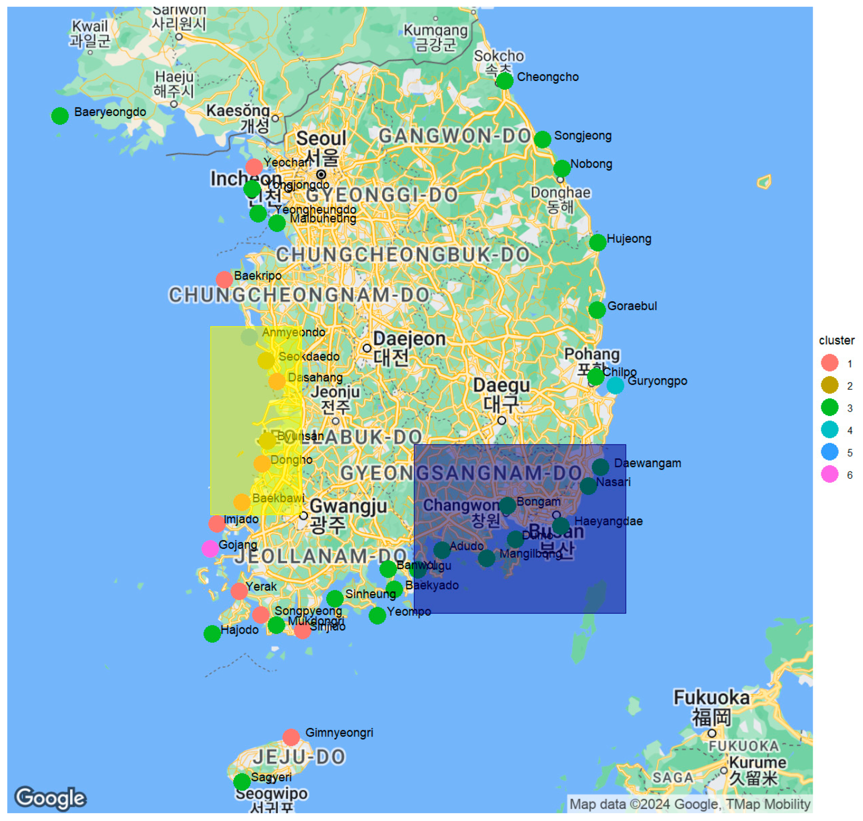
3.1. Coastal Waste Monitoring Data Clustering Result
3.2. Regression Models
3.2.1. Regression Models for South-Western Region
3.2.2. Regression Models for the South-Eastern Region
3.3. Model Validation
4. Discussion
5. Conclusions
Author Contributions
Funding
Institutional Review Board Statement
Informed Consent Statement
Data Availability Statement
Conflicts of Interest
References
- Gall, S.C.; Thompson, R.C. The impact of debris on marine life. Mar. Pollut. Bull. 2015, 92, 170–179. [Google Scholar] [CrossRef] [PubMed]
- Agamuthu, P.; Mehran, S.; Norkhairah, A.; Norkhairiyah, A. Marine debris: A review of impacts and global initiatives. Waste Manag. Res. 2019, 37, 987–1002. [Google Scholar] [CrossRef] [PubMed]
- Jang, Y.C.; Lee, J.; Hong, S.; Mok, J.Y.; Kim, K.S.; Lee, Y.J.; Choi, H.W.; Kang, H.; Lee, S. Estimation of the annual flow and stock of marine debris in South Korea for management purposes. Mar. Pollut. Bull. 2014, 86, 505–511. [Google Scholar] [CrossRef] [PubMed]
- McIlgorm, A.; Campbell, H.F.; Rule, M.J. The economic cost and control of marine debris damage in the Asia-Pacific region. Ocean Coast. Manag. 2011, 54, 643–651. [Google Scholar] [CrossRef]
- Ostle, C.; Thompson, R.C.; Broughton, D.; Gregory, L.; Wootton, M.; Johns, D.G. The rise in ocean plastics evidenced from a 60-year time series. Nat. Commun. 2019, 10, 8–13. [Google Scholar] [CrossRef]
- Jambeck, J.R.; Ji, Q.; Zhang, Y.-G.; Liu, D.; Grossnickle, D.M.; Luo, Z.-X. Plastic waste inputs from land into the ocean. Science 2015, 347, 764–768. [Google Scholar] [CrossRef] [PubMed]
- Niaounakis, M. The Problem of Marine Plastic Debris. In Management of Marine Plastic Debris; Elsevier: Amsterdam, The Netherlands, 2017; pp. 1–55. [Google Scholar]
- Wright, S.L.; Kelly, F.J. Plastic and Human Health: A Micro Issue? Environ. Sci. Technol. 2017, 51, 6634–6647. [Google Scholar] [CrossRef] [PubMed]
- Jones, M.M. Fishing debris in the Australian marine environment. Mar. Pollut. Bull. 1995, 30, 25–33. [Google Scholar] [CrossRef]
- McPhee, D.P.; Leadbitter, D.; Skilleter, G.A. Swallowing the bait: Is recreational fishing in Australia ecologically sustainable? Pac. Conserv. Biol. 2002, 8, 40. [Google Scholar] [CrossRef]
- Watson, A.R.; Blount, C.; McPhee, D.P.; Zhang, D.; Smith, M.P.L.; Reeds, K.; Williamson, J.E. Source, fate and management of recreational fishing marine debris. Mar. Pollut. Bull. 2022, 178, 113500. [Google Scholar] [CrossRef]
- Nash, A.D. Impacts of marine debris on subsistence fishermen: An exploratory study. Mar. Pollut. Bull. 1992, 24, 150–156. [Google Scholar] [CrossRef]
- Chiappone, M.; White, A.; Swanson, D.W.; Miller, S.L. Occurrence and biological impacts of fishing gear and other marine debris in the Florida Keys. Mar. Pollut. Bull. 2002, 44, 597–604. [Google Scholar] [CrossRef] [PubMed]
- Unger, A.; Harrison, N. Fisheries as a source of marine debris on beaches in the United Kingdom. Mar. Pollut. Bull. 2016, 107, 52–58. [Google Scholar] [CrossRef]
- Ramos, J.A.A.; Pessoa, W.V.N. Fishing marine debris in a northeast Brazilian beach: Composition, abundance and tidal changes. Mar. Pollut. Bull. 2019, 142, 428–432. [Google Scholar] [CrossRef]
- Consoli, P.; Romeo, T.; Angiolillo, M.; Canese, S.; Esposito, V.; Salvati, E.; Scotti, G.; Andaloro, F.; Tunesi, L. Marine litter from fishery activities in the Western Mediterranean sea: The impact of entanglement on marine animal forests. Environ. Pollut. 2019, 249, 472–481. [Google Scholar] [CrossRef]
- Edyvane, K.S.; Penny, S.S. Trends in derelict fishing nets and fishing activity in northern Australia: Implications for trans-boundary fisheries management in the shared Arafura and Timor Seas. Fish. Res. 2017, 188, 23–37. [Google Scholar] [CrossRef]
- Serra-Gonçalves, C.; Lavers, J.L.; Bond, A.L. Global Review of Beach Debris Monitoring and Future Recommendations. Environ. Sci. Technol. 2019, 53, 12158–12167. [Google Scholar] [CrossRef] [PubMed]
- National Coastal Waste Monitoring. Available online: https://www.meis.go.kr/mli/monitoringInfo/intro.do (accessed on 24 April 2023).
- Hafezi, M.H.; Daisy, N.S.; Liu, L. A Cluster-Based Technique for Identifying and Grouping Oily Waste Types Generated from Marine Oil Spill Response Operations. Front. Environ. Sci. 2022, 10, 910214. [Google Scholar] [CrossRef]
- Fauzan, A.; Fadillah, G.; Fitria, A.; Adriana, H.; Bariklana, M. Cluster Mapping of Waste Exposure Using DBSCAN Approach: Study of Spatial Patterns and Potential Distribution in Bantul Regency. JOIV Int. J. Inform. Vis. 2024, 8, 751. [Google Scholar] [CrossRef]
- Charrad, M.; Ghazzali, N.; Boiteau, V.; Niknafs, A. NbClust: An R Package for Determining the Relevant Number of Clusters in a Data Set. J. Stat. Softw. 2014, 61, 1–36. [Google Scholar] [CrossRef]
- Miaou, S. A stepwise time series regression procedure for water demand model identification. Water Resour. Res. 1990, 26, 1887–1897. [Google Scholar] [CrossRef]
- Akhter, N.; Malik, A.M.; Jamshaid, F.; Yasir, M.; Ayub, A.; Hussain, N. Time series model selection via stepwise regression to predict GDP Growth of Pakistan. Indian J. Econ. Bus. 2021, 20, 1881–1894. [Google Scholar]
- Salehi Sardoei, A.; Sharifani, M.; Khoshhal Sarmast, M.; Ghasemnejhad, M. Stepwise Regression Analysis of Citrus Genotype Under Cold Stress. Gene Cell Tissue 2022, 10, e126518. [Google Scholar] [CrossRef]
- Grömping, U. Relative Importance for Linear Regression in R: The Package relaimpo. J. Stat. Softw. 2006, 17, 1–27. [Google Scholar] [CrossRef]
- Pandit, V.; Khairullah, Z.Y. Stepwise Regression Choosing the Proper Level of Significance. In Proceedings of the 2015 Academy of Marketing Science, Bari, Italy, 14–18 July 2015; pp. 395–398. [Google Scholar]
- In Lee, K.; Koval, J.J. Determination of the best significance level in forward stepwise logistic regression. Commun. Stat.—Simul. Comput. 1997, 26, 559–575. [Google Scholar] [CrossRef]
- Wang, Q.; Koval, J.J.; Mills, C.A.; Lee, K.-I.D. Determination of the Selection Statistics and Best Significance Level in Backward Stepwise Logistic Regression. Commun. Stat.—Simul. Comput. 2007, 37, 62–72. [Google Scholar] [CrossRef]
- Ozili, P.K. The Acceptable R-Square in Empirical Modelling for Social Science Research. In Social Research Methodology and Publishing Results: A Guide to Non-Native English Speakers; IGI Global: Hershey, PA, USA, 2023; pp. 134–143. [Google Scholar]
- Hardesty, B.D.; Lawson, T.J.; van der Velde, T.; Lansdell, M.; Wilcox, C. Estimating quantities and sources of marine debris at a continental scale. Front. Ecol. Environ. 2017, 15, 18–25. [Google Scholar] [CrossRef]
- Hardesty, B.D.; Harari, J.; Isobe, A.; Lebreton, L.; Maximenko, N.; Potemra, J.; van Sebille, E.; Dick Vethaak, A.; Wilcox, C. Using numerical model simulations to improve the understanding of micro-plastic distribution and pathways in the marine environment. Front. Mar. Sci. 2017, 4, 30. [Google Scholar] [CrossRef]
- Lebreton, L.C.M.; Greer, S.D.; Borrero, J.C. Numerical modelling of floating debris in the world’s oceans. Mar. Pollut. Bull. 2012, 64, 653–661. [Google Scholar] [CrossRef]
- Kroon, F.; Motti, C.; Talbot, S.; Sobral, P.; Puotinen, M. A workflow for improving estimates of microplastic contamination in marine waters: A case study from North-Western Australia. Environ. Pollut. 2018, 238, 26–38. [Google Scholar] [CrossRef]


| Rank | Category 3 | Quantity | Proportion |
|---|---|---|---|
| 1 | Fragmentary Plastic Particles | 14,785 | 14.03% |
| 2 | Twisted Ropes (Fishing) | 13,592 | 12.90% |
| 3 | Beverage Bottles and Caps | 12,549 | 11.91% |
| 4 | Rigid Plastic Fragments | 12,080 | 11.46% |
| 5 | Styrofoam Buoys | 6058 | 5.75% |
| 6 | Vinyl Packaging (Ice Cream Wrappers, Snack Bags, etc.) | 4838 | 4.59% |
| 7 | Plastic Bags | 4588 | 4.35% |
| 8 | Film-type Plastic Fragments | 3656 | 3.47% |
| 9 | Cords (Packaging Cords) | 3471 | 3.29% |
| 10 | Miscellaneous Rigid Plastic | 2780 | 2.64% |
| 11 | Disposable Plates, Spoons, Straws, etc. | 2367 | 2.25% |
| 12 | Styrofoam Food Containers (Cup Noodles, Lunch Boxes, Fruit Packaging, etc.) | 2165 | 2.05% |
| 13 | Other Fragments | 2086 | 1.98% |
| 14 | Other Materials | 1919 | 1.82% |
| 15 | Cigarette Butts | 1855 | 1.76% |
| 16 | Fake Bait, Fluorescent Hooks, Fishing Bait Containers | 1583 | 1.50% |
| 17 | Other Fragmentary Plastic (Sponges, Disposable Wipes, etc.) | 1373 | 1.30% |
| 18 | Fiber-type Plastic Fragments | 1336 | 1.27% |
| 19 | Fishing Nets | 1308 | 1.24% |
| 20 | Synthetic Fiber (Clothing, Synthetic Fabric, Gloves, Socks, Blankets, etc.) | 1118 | 1.06% |
| 21 | Plastic Buoys | 1099 | 1.04% |
| 22 | Other Plastics | 1092 | 1.04% |
| 23 | Styrofoam Packaging Cushioning Material (Shock Absorbers for Electrical Appliances, etc.) | 1085 | 1.03% |
| 24 | Food Packaging Containers (Red Pepper Paste Tubes, Soy Sauce Bottles, etc.) | 756 | 0.72% |
| 25 | Lighters | 741 | 0.70% |
| 26 | Fireworks and Firework Accessories | 636 | 0.60% |
| 27 | Styrofoam Fishing Boxes | 596 | 0.57% |
| 28 | Fishing Lines | 566 | 0.54% |
| 29 | Film-type Plastics (Disposable Hygienic Gloves, etc.) | 417 | 0.40% |
| 30 | Toys, Dolls, Recreational Items, Office Supplies | 402 | 0.38% |
| 31 | Detergent Containers | 396 | 0.38% |
| 32 | Trap and Eel Trap Bait Containers | 373 | 0.35% |
| 33 | Fiber-type Plastics (Nets, Packaging Materials, etc.) | 365 | 0.35% |
| 34 | Packaging Bands (Wide, Hard Bands) | 234 | 0.22% |
| 35 | Pesticide Containers and Insecticides | 187 | 0.18% |
| 36 | Syringes | 146 | 0.14% |
| 37 | Various Vinyl Packaging | 135 | 0.13% |
| 38 | Buoys (Black) | 100 | 0.09% |
| 39 | Aquaculture Chemical Containers | 97 | 0.09% |
| 40 | Film-type Balloons | 96 | 0.09% |
| 41 | Various Styrofoam | 86 | 0.08% |
| 42 | Buoys (Round Bar, Large, Blue) | 83 | 0.08% |
| 43 | Buoys (Bar, Orange) | 72 | 0.07% |
| 44 | Medicine Bottles and Packaging, Syringes, etc. | 40 | 0.04% |
| 45 | Miscellaneous Rigid Buoys | 39 | 0.04% |
| 46 | Buoys (Oval, Blue) | 36 | 0.03% |
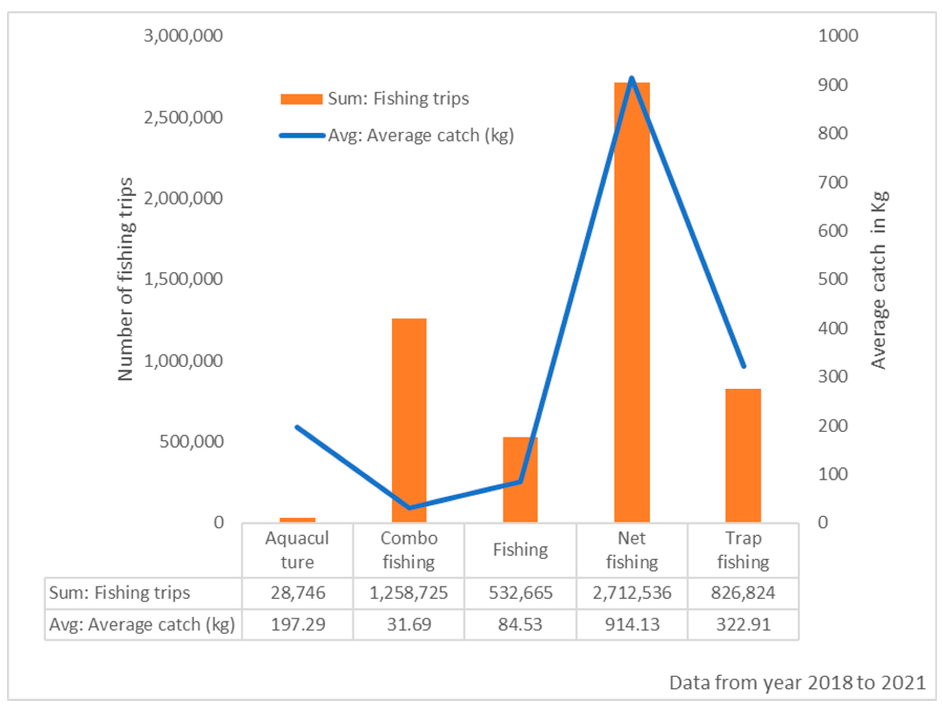
| Major Category | Sub-Category | Fishing Trips | Average Catch (kg/trip) |
|---|---|---|---|
| Aquaculture | Coastal Cage Farming | 6192 | 15.21 |
| Aquaculture | 22 | 15 | |
| Inland Tanks Aquaculture | 7 | 7.86 | |
| Inland Embankment Aquaculture | 12 | 1120 | |
| Cooperative Aquaculture | 363 | 10.24 | |
| Bottom Surface Aquaculture | 14,070 | 59.44 | |
| Hanging Aquaculture | 7359 | 214.26 | |
| Mixed Aquaculture | 721 | 136.33 | |
| Combo Fishing | Coastal Combo Fishing | 1,258,725 | 31.69 |
| Fishing | Offshore Longline Fishing | 179,454 | 200.51 |
| Offshore Single-line Fishing | 292 | 132.99 | |
| Fishing Vessels | 187,794 | 22.44 | |
| Fishing | 657 | 15.42 | |
| Coastal Single-line Fishing | 1 | 5 | |
| Jig Fishing | 164,467 | 130.8 | |
| Net Fishing | Fish Fence Fishing | 3902 | 65.59 |
| Anchovy Trawl Fishing | 72,313 | 921.97 | |
| Village Net Fishing | 8555 | 33.97 | |
| Offshore Stick-held Dip Net Fishing | 472 | 229.34 | |
| Large Purse Seines Fishery | 14,887 | 27,372.52 | |
| Small Purse Seines Fishery | 11,696 | 290.34 | |
| Coastal Seines Fishery | 30,273 | 179.18 | |
| Fyke Net Fishing | 3296 | 28.35 | |
| Funnel Net-type Fishing | 7148 | 26.45 | |
| Stow Net Fishing | 191,476 | 259.31 | |
| Coastal Improved Stow Net Fishing | 182,626 | 71.48 | |
| Coastal Stow Net Fishing | 209 | 39.05 | |
| Offshore Fixed Gill Net Fishing | 22,778 | 177.52 | |
| Offshore Drift Gill Net Fishing | 81,273 | 203.36 | |
| Offshore Gill Net Fishing | 174,209 | 251.76 | |
| Coastal Drift Gill Net Fishing | 772 | 46.71 | |
| Coastal Gill Net Fishing | 1,626,838 | 44.62 | |
| Winged Gape Net Fishing | 17,428 | 29.06 | |
| Long Bag Net-type Fishing | 607 | 23.49 | |
| Long Bag Net Fishing | 26,771 | 13.95 | |
| Gape Net Fishing | 10,353 | 20.38 | |
| Large Trawl Fishing | 467 | 1501.51 | |
| Eastern Sea Medium Single Trawl Fishing | 17,679 | 226 | |
| South-western Sea Medium Double Trawl Fishing | 14,201 | 707.08 | |
| South-western Sea Medium Single Trawl Fishing | 43,913 | 188.34 | |
| Large Double Seine Fishing | 39,644 | 1271.27 | |
| Large Single Seine Fishing | 47,363 | 197.25 | |
| Large Set Net Fishing | 4188 | 80.76 | |
| Small Set Net Fishing | 278 | 15.4 | |
| Set Net Fishing | 204 | 34.51 | |
| Medium Set Net Fishing | 1194 | 261.9 | |
| Large Trawl Fishing | 19,080 | 543.69 | |
| Eastern Sea Medium Trawl Fishing | 3461 | 683.51 | |
| Offshore Dredge Fishing | 29,952 | 197.9 | |
| Shellfish Dredge Fishing | 3030 | 144.67 | |
| Trap Fishing | Offshore Eel Trap Fishing | 57,988 | 420.18 |
| Offshore Trap Fishing | 106,477 | 820.51 | |
| Coastal Trap Fishing | 662,358 | 40.94 | |
| Trap Fishing | 1 | 10 |
| Variables | Description |
|---|---|
| y | Total fishing activity-induced coastal waste |
| n_avg | Average catch per trip for net fishing |
| n_cnt | Number of net fishing trips |
| f_avg | Average catch per trip for hook and line fishing |
| f_cnt | Number of hook and line fishing trips |
| a_avg | Average catch per trip for aquaculture |
| a_cnt | Number of aquaculture trips |
| c_avg | Average catch per trip for combo fishing |
| c_cnt | Number of combo fishing trips |
| Variable | Coefficient | Standard Error | t-Value | Pr(>|t|) |
|---|---|---|---|---|
| Constant | 2.01837 | 0.43526 | 4.637 | 1.05 × 10⁻⁵ |
| c_avg0 | −4.00705 | 2.67794 | −1.496 | 0.1377 |
| n_cnt0 | −0.06205 | 0.03367 | −1.843 | 0.0683 |
| f_cnt0 | −0.46605 | 0.19337 | −2.41 | 0.0177 |
| a_cnt0 | −0.05613 | 0.03452 | −1.626 | 0.1071 |
| c_cnt0 | 0.19638 | 0.08085 | 2.429 | 0.0169 |
| R-squared | 0.1676 | |||
| Adjusted R-squared | 0.1268 | |||
| Variable | Coefficient | Standard Error | t-Value | Pr (>|t|) |
|---|---|---|---|---|
| Constant | 1.54244 | 0.70146 | 2.199 | 3.06 × 10⁻² |
| f_avg0 | 3.60321 | 1.67136 | 2.156 | 0.033887 |
| f_cnt0 | 1.09048 | 0.35482 | 3.073 | 0.002835 |
| c_cnt0 | −0.20683 | 0.057 | −3.628 | 0.000483 |
| c_avg1 | −14.2267 | 3.60502 | −3.946 | 0.000162 |
| f_cnt1 | −0.86617 | 0.31472 | −2.752 | 0.007219 |
| f_avg2 | 6.4558 | 1.71564 | 3.763 | 0.000306 |
| a_avg2 | −0.13617 | 0.08158 | −1.669 | 0.098727 |
| f_cnt2 | −0.99735 | 0.40359 | −2.471 | 0.015438 |
| a_cnt2 | −0.05832 | 0.02823 | −2.066 | 0.04185 |
| c_cnt2 | 0.37377 | 0.09246 | 4.043 | 0.000115 |
| n_avg3 | −5.36948 | 1.39558 | −3.847 | 0.000229 |
| f_avg3 | 2.66226 | 1.73349 | 1.536 | 0.128264 |
| a_avg3 | −0.17988 | 0.08662 | −2.077 | 0.040817 |
| f_cnt3 | 0.9043 | 0.36743 | 2.461 | 0.015848 |
| c_cnt3 | −0.39833 | 0.08913 | −4.469 | 2.38 × 10⁻⁵ |
| f_avg4 | 3.4314 | 1.62741 | 2.109 | 0.037896 |
| n_cnt4 | −0.36898 | 0.07079 | −5.213 | 1.26 × 10⁻⁶ |
| c_cnt4 | 0.90432 | 0.16284 | 5.554 | 3.07 × 10⁻⁷ |
| c_avg5 | −5.63903 | 3.5253 | −1.6 | 1.13 × 10⁻¹ |
| n_cnt5 | 0.07798 | 0.04436 | 1.758 | 8.23 × 10⁻² |
| a_cnt5 | −0.07323 | 0.0317 | −2.31 | 2.33 × 10⁻² |
| R-squared | 0.544 | |||
| Adjusted R-squared | 0.4326 | |||
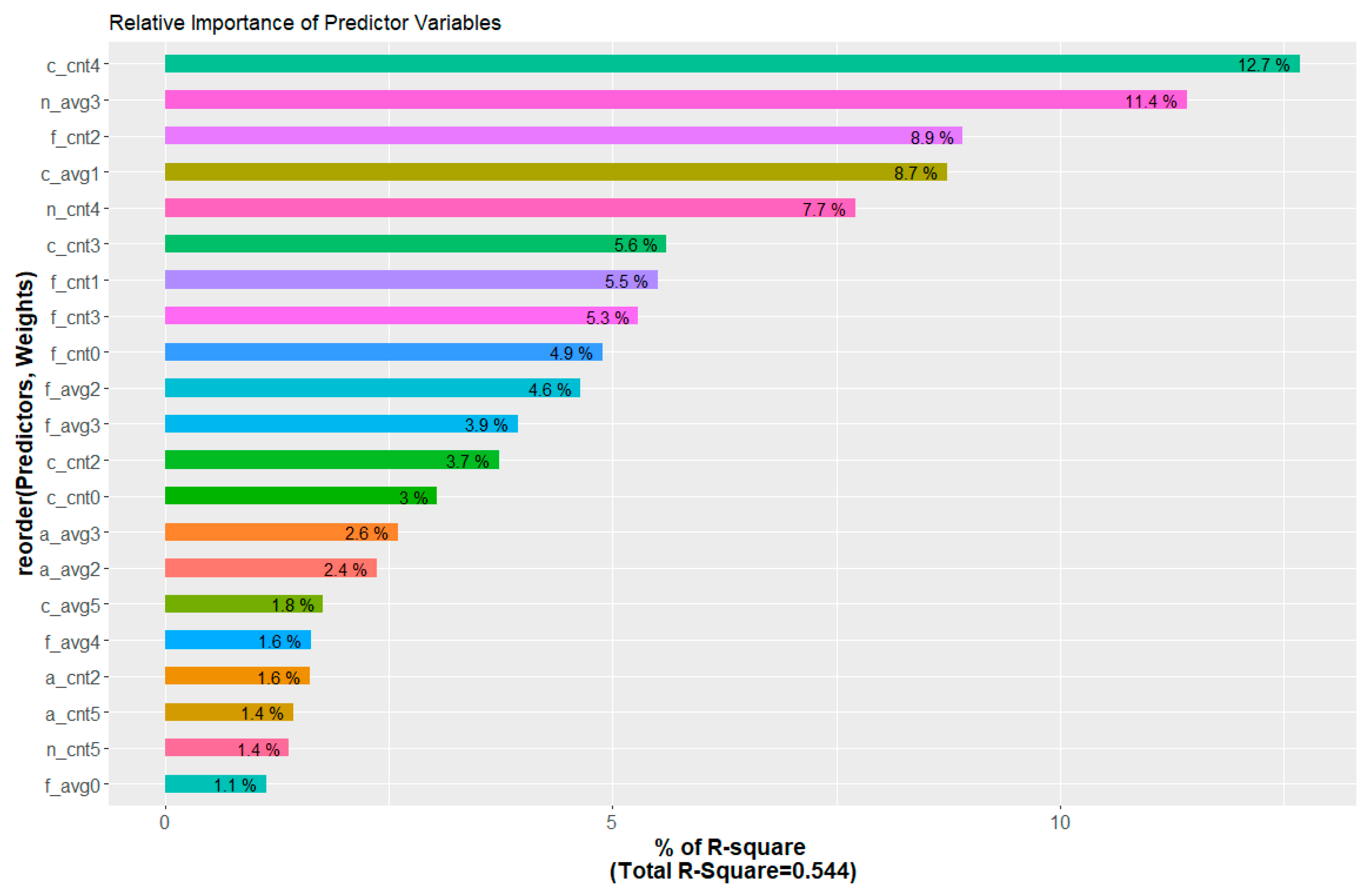
| Fishing Method | Variables | Relative Importance | Sub-Total |
|---|---|---|---|
| Aquaculture | a_avg2 | 2.4 | 8 |
| a_avg3 | 2.6 | ||
| a_cnt2 | 1.6 | ||
| a_cnt5 | 1.4 | ||
| Combo Fishing | c_avg1 | 8.7 | 35.5 |
| c_avg5 | 1.8 | ||
| c_cnt0 | 3 | ||
| c_cnt2 | 3.7 | ||
| c_cnt3 | 5.6 | ||
| c_cnt4 | 12.7 | ||
| Fishing | f_avg0 | 1.1 | 35.8 |
| f_avg2 | 4.6 | ||
| f_avg3 | 3.9 | ||
| f_avg4 | 1.6 | ||
| f_cnt0 | 4.9 | ||
| f_cnt1 | 5.5 | ||
| f_cnt2 | 8.9 | ||
| f_cnt3 | 5.3 | ||
| Net Fishing | n_avg3 | 11.4 | 20.5 |
| n_cnt4 | 7.7 | ||
| n_cnt5 | 1.4 |
| Time Period | Variables | Relative Importance | Sub-Total |
|---|---|---|---|
| 0 (no time difference) | c_cnt0 | 3 | 9 |
| f_avg0 | 1.1 | ||
| f_cnt0 | 4.9 | ||
| 1 (two months earlier) | c_avg1 | 8.7 | 14.2 |
| f_cnt1 | 5.5 | ||
| 2 (four months earlier) | a_avg2 | 2.4 | 21.2 |
| a_cnt2 | 1.6 | ||
| c_cnt2 | 3.7 | ||
| f_avg2 | 4.6 | ||
| f_cnt2 | 8.9 | ||
| 3 (six months earlier) | a_avg3 | 2.6 | 28.8 |
| c_cnt3 | 5.6 | ||
| f_avg3 | 3.9 | ||
| f_cnt3 | 5.3 | ||
| n_avg3 | 11.4 | ||
| 4 (eight months earlier) | c_cnt4 | 12.7 | 22 |
| f_avg4 | 1.6 | ||
| n_cnt4 | 7.7 | ||
| 5 (ten months earlier) | a_cnt5 | 1.4 | 4.6 |
| c_avg5 | 1.8 | ||
| n_cnt5 | 1.4 |
| Variable | Coefficient | Standard Error | t-Value | Pr(>|t|) |
|---|---|---|---|---|
| Constant | 2.74823 | 0.51673 | 5.319 | 4.81 × 10⁻⁷ |
| f_avg0 | 2.16237 | 1.417 | 1.526 | 0.1296 |
| a_avg0 | −0.15551 | 1.06117 | −2.542 | 0.0123 |
| c_avg0 | −4.11147 | 2.05385 | −2.002 | 0.0475 |
| R-squared | 0.07815 | |||
| Adjusted R-squared | 0.05548 | |||
| Variable | Coefficient | Standard Error | t-Value | Pr(>|t|) |
|---|---|---|---|---|
| Constant | 16.35444 | 6.75476 | 2.421 | 1.72 × 10⁻² |
| n_avg0 | 3.9317 | 2.31056 | 1.702 | 0.091843 |
| a_avg0 | −0.13713 | 0.08315 | −1.648 | 0.102168 |
| a_cnt0 | 0.44985 | 0.14135 | 3.182 | 0.001931 |
| n_avg1 | 14.62571 | 4.56619 | 3.203 | 0.00181 |
| c_avg1 | −6.92424 | 2.23576 | −3.097 | 0.002519 |
| n_cnt1 | −0.01673 | 0.01187 | −1.41 | 0.161514 |
| a_cnt1 | −0.34899 | 0.11884 | −2.937 | 0.004092 |
| c_cnt1 | 0.8321 | 0.27576 | 3.018 | 0.003211 |
| n_avg2 | −6.5311 | 4.09674 | −1.594 | 0.113951 |
| f_avg2 | −3.39125 | 1.84694 | −1.836 | 0.069221 |
| c_avg3 | 3.79867 | 2.90096 | 1.309 | 0.193295 |
| n_cnt3 | 0.02487 | 0.01502 | 1.656 | 0.100844 |
| f_cnt3 | 2.42366 | 1.7821 | 1.36 | 0.176797 |
| a_cnt3 | −0.19956 | 0.10653 | −1.873 | 0.63852 |
| c_cnt3 | −0.54821 | 0.15758 | −3.479 | 0.000739 |
| n_avg4 | 10.46709 | 4.20227 | 2.491 | 0.014343 |
| f_avg4 | 3.1383 | 2.00603 | 1.564 | 0.120784 |
| a_avg4 | −0.11951 | 0.06563 | −1.821 | 0.071519 |
| c_avg4 | −13.53992 | 4.62505 | −2.928 | 0.004206 |
| a_avg5 | −0.17262 | 0.07571 | −2.28 | 0.024674 |
| f_cnt5 | 4.91696 | 1.84864 | 2.66 | 0.00907 |
| a_cnt5 | −0.21667 | 0.12104 | −1.79 | 0.076386 |
| R-squared | 0.5105 | |||
| Adjusted R-squared | 0.4059 | |||
| Fishing Method | Variables | Relative Importance | Sub-Total |
|---|---|---|---|
| Aquaculture | a_avg0 | 1.9 | 50.5 |
| a_avg4 | 9.1 | ||
| a_avg5 | 10.1 | ||
| a_cnt0 | 5.1 | ||
| a_cnt1 | 7.6 | ||
| a_cnt3 | 4.6 | ||
| a_cnt5 | 12.1 | ||
| Combo Fishing | c_avg1 | 7.4 | 19 |
| c_avg3 | 1.2 | ||
| c_avg4 | 3.6 | ||
| c_cnt1 | 3.2 | ||
| c_cnt3 | 3.6 | ||
| Fishing | f_avg2 | 2 | 14.4 |
| f_avg4 | 2.2 | ||
| f_cnt3 | 2.3 | ||
| f_cnt5 | 7.9 | ||
| Net Fishing | n_avg0 | 2.1 | 16.2 |
| n_avg1 | 2.6 | ||
| n_avg2 | 4.4 | ||
| n_avg4 | 4.2 | ||
| n_cnt1 | 1.3 | ||
| n_cnt3 | 1.6 |
| Time Period | Variables | Relative Importance | Sub-Total |
|---|---|---|---|
| 0 (no time difference) | a_avg0 | 1.9 | 9.1 |
| a_cnt0 | 5.1 | ||
| n_avg0 | 2.1 | ||
| 1 (two months earlier) | a_cnt1 | 7.6 | 22.1 |
| c_avg1 | 7.4 | ||
| c_cnt1 | 3.2 | ||
| n_avg1 | 2.6 | ||
| n_cnt1 | 1.3 | ||
| 2 (four months earlier) | f_avg2 | 2 | 6.4 |
| n_avg2 | 4.4 | ||
| 3 (six months earlier) | a_cnt3 | 4.6 | 13.3 |
| c_avg3 | 1.2 | ||
| c_cnt3 | 3.6 | ||
| f_cnt3 | 2.3 | ||
| n_cnt3 | 1.6 | ||
| 4 (eight months earlier) | a_avg4 | 9.1 | 19.1 |
| c_avg4 | 3.6 | ||
| f_avg4 | 2.2 | ||
| n_avg4 | 4.2 | ||
| 5 (ten months earlier) | a_avg5 | 10.1 | 30.1 |
| a_cnt5 | 12.1 | ||
| f_cnt5 | 7.9 |
| South-Western Region | South-Eastern Region | ||||
|---|---|---|---|---|---|
| Mean of x | t-Value | p-Value | Mean of x | t-Value | p-Value |
| 1.27 × 10⁻¹⁵ | 7.86 × 10⁻¹⁶ | 1 | 1.33 × 10⁻¹⁶ | 6.57 × 10⁻¹⁶ | 1 |
Disclaimer/Publisher’s Note: The statements, opinions and data contained in all publications are solely those of the individual author(s) and contributor(s) and not of MDPI and/or the editor(s). MDPI and/or the editor(s) disclaim responsibility for any injury to people or property resulting from any ideas, methods, instructions or products referred to in the content. |
© 2024 by the authors. Licensee MDPI, Basel, Switzerland. This article is an open access article distributed under the terms and conditions of the Creative Commons Attribution (CC BY) license (https://creativecommons.org/licenses/by/4.0/).
Share and Cite
Lee, S.-H.; Hong, S.-K.; Lee, J.; Yu, J.-W.; Kim, H.-T.; Joung, T.-H. Estimating the Temporal Impacts of Nearshore Fisheries on Coastal Ocean-Sourced Waste Accumulation in South Korea Using Stepwise Regression. Sustainability 2024, 16, 5663. https://doi.org/10.3390/su16135663
Lee S-H, Hong S-K, Lee J, Yu J-W, Kim H-T, Joung T-H. Estimating the Temporal Impacts of Nearshore Fisheries on Coastal Ocean-Sourced Waste Accumulation in South Korea Using Stepwise Regression. Sustainability. 2024; 16(13):5663. https://doi.org/10.3390/su16135663
Chicago/Turabian StyleLee, Seung-Hyun, Seung-Kweon Hong, Jongsung Lee, Ji-Won Yu, Hong-Tae Kim, and Tae-Hwan Joung. 2024. "Estimating the Temporal Impacts of Nearshore Fisheries on Coastal Ocean-Sourced Waste Accumulation in South Korea Using Stepwise Regression" Sustainability 16, no. 13: 5663. https://doi.org/10.3390/su16135663
APA StyleLee, S.-H., Hong, S.-K., Lee, J., Yu, J.-W., Kim, H.-T., & Joung, T.-H. (2024). Estimating the Temporal Impacts of Nearshore Fisheries on Coastal Ocean-Sourced Waste Accumulation in South Korea Using Stepwise Regression. Sustainability, 16(13), 5663. https://doi.org/10.3390/su16135663