Abstract
Geotechnical site characterizations aim to determine site-specific subsurface profiles and provide a comprehensive understanding of associated soil properties, which are important for geotechnical engineering design. Traditional methods often neglect the inherent cross-correlations among different soil properties, leading to high bias in site characterization interpretations. This paper introduces a novel data-driven site characterization (DDSC) method that employs the Bayesian-optimized multi-output Gaussian process (BO-MOGP) to capture both the spatial correlations across different site locations and the cross-correlations among various soil properties. By considering the dual-correlation feature, the proposed BO-MOGP method enhances the accuracy of predictions of soil properties by leveraging information as much as possible across multiple soil properties. The superiority of the proposed method is demonstrated through a simulated example and the case study of a Taipei construction site. These examples illustrate that the proposed BO-MOGP method outperforms traditional methods that fail to consider both types of correlations, as evidenced by the reduced prediction uncertainty and the accurate identification of cross-correlations. Furthermore, the ability of the proposed BO-MOGP method to generate conditional random fields supports its effectiveness in geotechnical site characterizations.
1. Introduction
Geotechnical materials, unlike their artificial counterparts, are inherently unpredictable [1]. While artificial materials benefit from the predictability and uniformity afforded by controlled manufacturing processes, geotechnical materials are shaped by eons of geological processes [2,3,4]. These natural processes, including sedimentary deposition, erosion, and tectonic shifts, contribute to a diverse array of materials with varied properties. This diversity results from the intricate interplay of geological forces over time, leading to a mosaic of material compositions across different geographic and stratigraphic layers. Constitutive equations, the mathematical tools engineers use to predict material behavior under different stress conditions, often fall short of accounting for the full complexity of these materials due to inherent biases. This discrepancy arises from the formation processes where sedimentary and tectonic activities introduce uneven distribution of matrix materials into the geotechnical composition [5]. The spatial variability of geotechnical materials complicates direct observation and understanding, rendering exploration methods like boreholes and geophysical surveys challenging. These approaches are foundational to engineering practice, offering a means to probe and assess subsurface profiles. While extensive borehole drilling and high-precision geophysical methods can provide detailed subsurface insights, they often come at prohibitive costs [6]. Consequently, engineering projects frequently rely on more economical, albeit less comprehensive, site investigation techniques. This reliance leads to a paradox where, despite the expertise of geotechnical engineers, the understanding of subsurface profiles remains incomplete, potentially compromising the integrity and safety of engineering projects.
In response to the challenges posed by the limitations of traditional site characterization methods, Phoon et al. [7] have proposed a data-driven approach termed data-driven site characterization (DDSC). This innovative methodology distinguishes itself by relying solely on measured data for site characterization. It encompasses not only the site-specific data collected for the current project but also incorporates existing data from various sources, including past projects at the same site, neighboring sites, or even data from distant locations [8]. DDSC marks a significant paradigm shift in the field of site characterization. Traditional methods typically depend on direct exploration techniques, which can be time-consuming and costly and often provide limited information about subsurface conditions. In contrast, DDSC capitalizes on the wealth of measured data available from diverse sources [9]. By employing advanced statistical and machine learning techniques, DDSC can effectively interpret sparse data sets, enabling the estimation of the spatial variability of subsurface soil with greater accuracy and from fewer data points. One of the key strengths of DDSC is its ability to integrate selective measurements with a broader range of data sources [10]. This approach allows for a more comprehensive understanding of subsurface conditions. For instance, selective measurements can be combined with geophysical survey data, historical borehole logs, and other relevant information to create a detailed and accurate characterization of the site. The adoption of DDSC brings many benefits. Firstly, it can enhance the accuracy of site characterizations by extracting as much information as possible from site investigation data. Secondly, it has the potential to significantly reduce the uncertainties for site characterization as it minimizes the need for extensive direct exploration. Lastly, the financial costs associated with site characterization can be substantially lowered, as DDSC maximizes the use of existing data and minimizes the need for new data collection [11].
In recent years, various methods have been developed for DDSC to address the challenges posed by the complex and often incomplete nature of geotechnical data. These methods aim to use the limited data available from site investigations to create accurate and reliable models of subsurface conditions. Ching and Phoon [12] developed the MUSIC method for DDSC. The acronym MUSIC stands for Multivariate, Uncertain and unique, Sparse, and InComplete, which aptly describes the common attributes of real-world site investigation data. The MUSIC method is specifically designed to handle these characteristics, providing a comprehensive framework for integrating and analyzing diverse data types to improve site characterization. Building on the foundations of the MUSIC method, Ching and Phoon [13] further developed the MUSIC-X method, where the “X” signifies the incorporation of spatial correlations. This extension of the original MUSIC approach considers spatial relationships across different locations, which is essential for capturing the spatial variability of subsurface conditions. By considering these spatial correlations, the MUSIC-X method offers a more refined and accurate characterization of the subsurface, thereby enhancing the reliability of geotechnical models. In parallel, Wang and Zhao [14,15] explored a new sampling paradigm from digital signal processing called compressive sampling (CS). This innovative approach can reconstruct a near replica of the original signal from a small number of measurements, making it particularly suitable for dealing with sparse geotechnical data. Compressive sampling provides a means to efficiently gather and process information from limited site investigations, offering a potential solution to the challenge of data scarcity in geotechnical engineering. Further expanding on the concept of compressive sampling, Wang et al. [16] developed a Bayesian CS–Karhunen–Loève (BCS-KL) expansion method. This method can generate random field samples (RFSs) directly from sparse measurements, providing a powerful tool for modeling the spatial variability of subsurface properties. Recent advancements in DDSC methods have also made strides in utilizing monitoring data, particularly for site uncertainty quantification. The monitoring of data, such as unsaturated hydraulic parameters for rainfall-induced slope failure, provides the benefit of enhancing our understanding of site conditions through Bayesian back analysis. Yang and Zhang [17] provided a comprehensive review on Bayesian back analysis of unsaturated hydraulic parameters for rainfall-induced slope failure, highlighting the importance of monitoring data in site uncertainty quantification. Rana and Sivakumar Babu [18] demonstrated the use of multi-output least square support vector regression (MLS-SVR) for Bayesian back analysis of rainfall-induced slope failure, further illustrating the role of monitoring data in improving the accuracy of DDSC methods.
Traditional methods for DDSC typically require abundant data to yield accurate and reliable results. These methods may struggle to provide precise characterizations of subsurface conditions when data are sparse or incomplete, and they may not effectively utilize the information contained in limited data sets. Conversely, Gaussian process (GP) offers a robust and flexible approach to address the challenges posed by the MUSIC characteristics of subsurface data. The GP model employs the kernel strategy to model the spatial correlations between any two points in the subsurface domain. This flexibility is paramount for geotechnical engineering applications, where soil properties can exhibit significant variability over short distances [19,20]. Unlike the fixed structures or assumptions inherent in methods like the BCS-KL expansion, GP’s kernel strategies can adapt to reflect the actual spatial continuity observed in geotechnical data. Furthermore, GP kernel strategies can be tailored to match the specific statistical properties of soil. This customization is achieved by selecting or designing kernel functions that best represent the spatial relationships and variability patterns of subsurface materials, thus providing a more accurate and representative model of soil properties [21]. Yoshida et al. [22] proposed a method for simultaneously estimating the trend and random component of soil properties at arbitrary locations using GP with the superposition of multiple Gaussian random fields. This approach allows for a more nuanced modeling of soil properties, considering both the underlying trends and the stochastic nature of the data. The use of GP has been instrumental in advancing the understanding and estimation of the spatial variability inherent to subsurface soil conditions. By conceptualizing the spatial variability of subsurface soil as a probabilistic model, GP treats soil properties, such as soil density, moisture content, and shear strength, as variables that follow a normal distribution. This approach is underpinned by the assumption that these soil properties, when observed at various spatial locations, collectively conform to a multivariate normal distribution. This powerful statistical framework enables the GP model to provide estimates of soil properties across different spatial domains, offering a mathematically rigorous method for predicting soil properties in areas that are not directly observed or measured [23]. The strength of the GP model lies in its flexibility and the depth of insight it provides into the spatial structure of subsurface soil variability. By employing a covariance function, the GP model can quantify the degree of similarity or correlations among different soil properties at different locations, thereby capturing the essence of spatial continuity and variability in subsurface materials.
The GP model has limitations despite its strengths. A significant challenge arises from the formulation of GP model, which tends to treat each soil property independently, without considering the potential cross-correlations among different soil properties [24]. Subsurface soil properties are often interrelated, where changes in one parameter could influence or indicate changes in another [25,26]. For example, soil density might have a direct relationship with moisture content, and ignoring such relationships could lead to an incomplete or skewed understanding of subsurface conditions. This isolationist approach becomes particularly problematic when dealing with sparse data sets, a common scenario in geotechnical engineering due to the logistical and financial constraints associated with collecting subsurface data. Parameters that are measured infrequently or at a limited number of locations are at a disadvantage, as the GP model does not use the potentially rich information available from more frequently measured parameters [27]. This can result in a significant loss of information, undermining the model’s predictive accuracy and leading to less reliable estimations of soil properties. One more limitation of the GP model is the determination of its hyperparameters. The objective function for hyperparameter tuning, often based on maximizing the marginal likelihood of the training data, is typically non-convex. This means there are multiple local maxima, making it challenging to find the global optimum.
In view of these limitations, this paper introduces a novel DDSC method that employs Bayesian-optimized MOGP (BO-MOGP) to overcome the shortcomings of the traditional GP model. The proposed BO-MOGP method captures both spatial correlations across different locations and cross-correlations among various soil properties. By considering the interdependencies among different soil properties, the proposed BO-MOGP method enhances the predictive accuracy of soil property estimations. This approach not only provides a more comprehensive understanding of subsurface conditions but also improves the reliability of geotechnical site characterizations, especially in cases where data are sparse. The remainder of this paper is structured as follows. Section 1 introduces the multi-output Gaussian process. Section 2 introduces the Bayesian optimization procedure. The presentation of the proposed BO-MOGP model is provided in Section 3. It is followed by verifying the proposed BO-MOGP method by a synthetic case and a real-world case in Section 4. This paper ends up with a conclusion in Section 5.
2. Multi-Output Gaussian Process
The GP is a probabilistic model used for regression tasks. It provides a flexible approach for modeling complex relationships in geotechnical data, allowing for the quantification of uncertainty in predictions.
The GP model is formulated as follows [28,29]:
where f represents the vector of soil properties at observed locations, modeled as random variables. The notation (·) signifies a multivariate normal distribution, with 0 being a vector of zeros that denotes the mean of the distribution. This assumption of a zero mean simplifies the model by reducing the number of parameters that need to be estimated, making the model more tractable and easier to work with. It also reflects a neutral prior belief, indicating that before observing any data, there is no specific expectation about the values of the soil properties. The term Q denotes the covariance matrix of the soil properties at observed locations, capturing the relationships and dependencies among different points in the geotechnical data.
The joint distribution for soil properties across observed and unobserved locations is given by a multivariate normal distribution:
where f* denotes the vector of soil properties at unobserved locations, Q** is the covariance matrix for soil properties at unobserved locations, Qf* is the cross-covariance matrix between the soil properties at observed and unobserved locations, and Q*f is the transpose of Qf*.
The posterior distribution for the soil properties at unobserved locations, conditioned on the soil properties at observed locations, is given by [30]:
where (·)−1 denotes the inverse of a matrix.
The matrix Q is defined by a Whittle–Matern (W-M) autocorrelation model due to its greater flexibility in modeling the spatial correlations in geotechnical data. The W-M kernel is particularly advantageous because it includes a parameter that controls the smoothness of the function, allowing it to better adapt to different types of spatial variability observed in soil properties. The W-M autocorrelation model is defined as follows [13]:
where xi and xj are the coordinates of the i-th and j-th location, respectively; ν is the sample smoothness parameter; δ is the scale of fluctuation (SOF); Γ(∙) is the gamma function; and Kν is the modified Bessel function of the second kind with order ν.
The hyperparameters (i.e., ν and δ) are optimized through the maximum likelihood method, with the corresponding log-likelihood function integral to this optimization [31]:
where (·)T denotes the transpose of a matrix, |·| represents the determinant of a matrix, and n is the number of unobserved locations.
Maximizing the log-likelihood function concerning ν and δ yields the optimal hyperparameters (i.e., ν* and δ*) as follows:
The MOGP is an extension of the GP model and is designed to handle multiple correlated output variables simultaneously. While a standard GP models a single output variable, an MOGP can model several outputs, capturing not only the relationships within each output but also the cross-correlations among different outputs [32]. In geotechnical engineering, it is often necessary to predict multiple interrelated soil properties. For example, soil stiffness, permeability, and strength are all important properties that can influence the behavior of soil and rock in various engineering applications, such as the design of foundations, tunnels, and retaining structures. These parameters are typically influenced by the same set of inputs, such as soil type, moisture content, and compaction level. MOGPs are particularly useful in this context because they can model multiple outputs simultaneously while capturing the correlations among them. This is important because the soil properties are often not independent; for instance, soil stiffness and strength might be related, as both can be affected by factors like soil density and composition [33]. By modeling these parameters together in an MOGP framework, one can use the information from one parameter to improve the predictions of another. For example, if there are measurements of soil stiffness at certain locations, and it is know that there is a correlation between soil stiffness and strength, one can use this information to improve predictions of soil strength at other locations, even if there are no direct measurements of strength at those locations. This can lead to more accurate and reliable predictions, which are crucial for making informed decisions in geotechnical engineering projects.
Mathematically, the MOGP is utilized to model all of the m soil properties simultaneously for each input location x, as follows:
where fi(x) is a row vector representing the i-th soil property.
The prior distribution over the m-output functions f(x) is Gaussian with zero mean vector 0 and a block-covariance matrix G as follows [34]:
where ⊗ denotes the Kronecker production, and P represents the covariance matrix across soil properties.
Here, G is a block matrix where each block Gij is a covariance matrix between outputs i and j and is derived by the Kronecker product of the matrix P and the matrix Q. The element of the matrix P(i, j) denotes the cross-correlations between the i-th output variable and the j-th output variable, and the element of the matrix Q(i, j) denotes the spatial correlations between the i-th unobserved location and the j-th unobserved location. The matrix P is a m × m semi-positive symmetrical matrix, and the matrix Q is a n × n symmetrical matrix consisting of the m soil properties at n unobserved locations; thus, the block-covariance matrix G is an mn × mn symmetrical matrix. The block matrix G is shown as follows:
The joint distribution of the soil properties at observed locations and unobserved locations is given by a multivariate normal distribution [35]:
where G** is the covariance matrix of the soil properties at unobserved locations, Gf* is the cross-covariance matrix between the soil properties at observed and unobserved locations, and G*f = Gf*T.
The posterior distribution for the soil properties at unobserved locations x*, conditioned on the soil properties at observed locations, is given by:
The hyperparameters need to be estimated efficiently to optimize the performance of MOGPs. These hyperparameters include ν and δ in the covariance function and elements in the matrix P and are represented as θ. In this study, the maximum likelihood method is employed to determine these hyperparameters by maximizing the likelihood of the soil properties at the observed locations [34].
Given that the joint distribution of soil properties at observed locations is Gaussian, the log-likelihood function L(ν, δ, P) can be expressed as follows:
Maximizing the log-likelihood function concerning ν, δ, and P yields the optimal hyperparameters as follows [36]:
3. Bayesian Optimization
Bayesian optimization is an essential technique for optimizing objective functions that are expensive to evaluate. It employs a surrogate model to approximate the unknown objective function, thereby enabling efficient navigation through the hyperparameter space. This strategy is important for MOGPs due to their complex and computationally intensive nature, where direct evaluations can be prohibitive. In this context, the surrogate model employed is the Student-t process, which offers advantages in terms of robustness to noise and handling outliers, making it suitable for environments where data may not strictly adhere to normality.
The objective function in this context is the log-likelihood function L(θ) of the MOGP, which is the log-likelihood of the observed soil properties under the current model’s configuration. The Student-t process utilized as a surrogate is characterized by a zero mean function m(θ), under the assumption of no prior knowledge, and a covariance function k(θi, θj). The formulation of the Student-t process can be expressed as follows:
where TP denotes the Student-t process and η represents the degrees of freedom, which influence the tail heaviness, providing flexibility in modeling distributions with heavier tails than those assumed by GPs.
The acquisition function used to guide the selection of new hyperparameters is the expected improvement (EI), which is particularly adapted for a Student-t surrogate model. The EI for a Student-t process is calculated based on the predictive distribution derived from the surrogate, focusing on areas of the hyperparameter space that promise the greatest potential improvement over the current best observation θ+. The EI can be mathematically described as
where θ+ is the location of the current best observation, and t(θ) represents the function’s value predicted by the Student-t process at new candidate points.
The optimization cycle proceeds by using the EI to select new hyperparameters for evaluation. The MOGP model is then run with these parameters, and the resulting value of the objective function is used to update the Student-t surrogate model. The surrogate’s parameters are updated by re-fitting to include the new set (ν, δ, P, L), incorporating the latest observations into the model. This iterative process is repeated until a satisfactory level of convergence is achieved or a predefined number of iterations is reached.
4. Proposed BO-MOGP for Site Characterizations
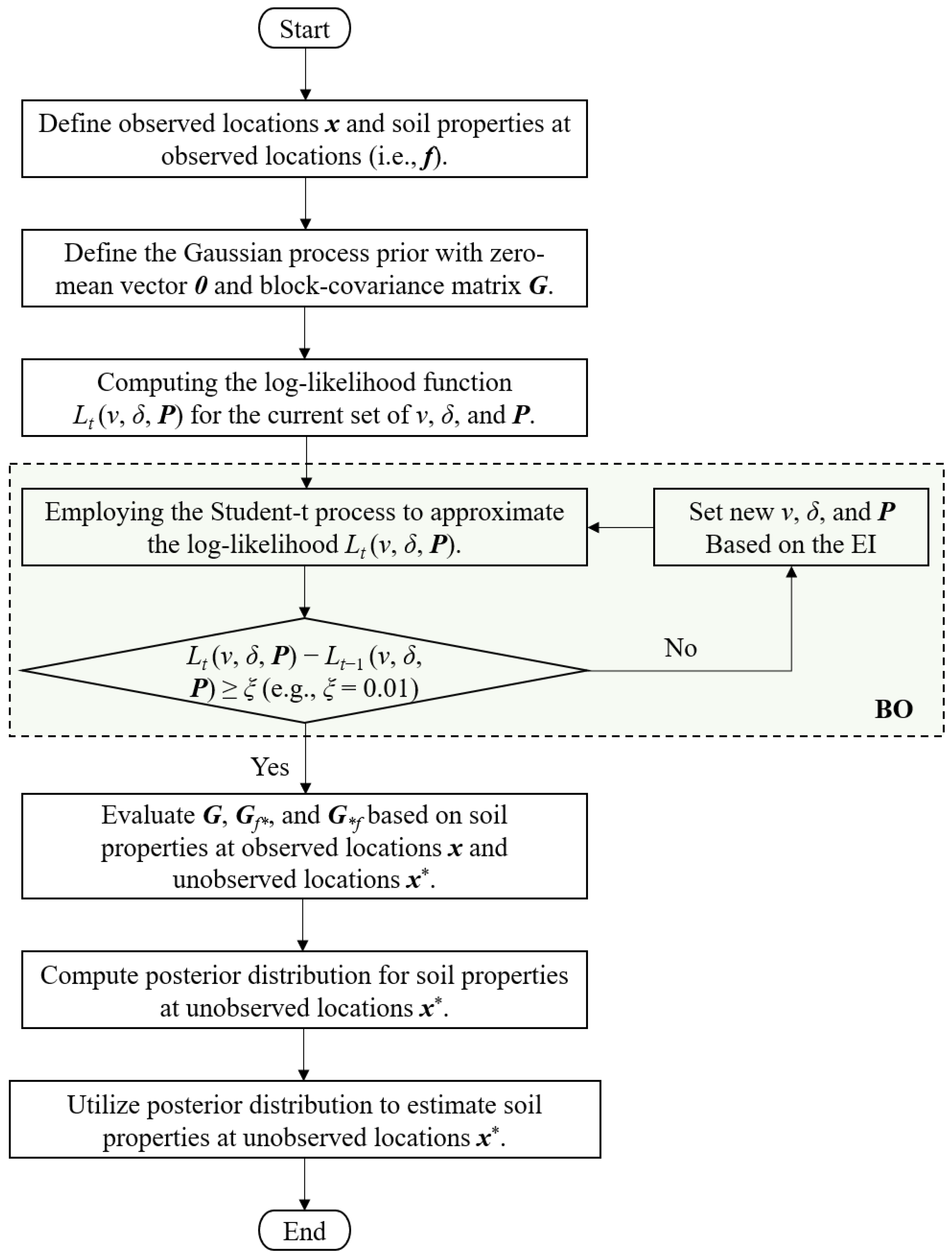
The proposed BO-MOGP method uses the strengths of both MOGP and BO to create a highly adaptive model that can dynamically incorporate new data and refine predictions based on the evolving understanding of the site conditions. This method is particularly effective in geotechnical engineering where the spatial correlations and the interdependencies among various soil properties can significantly influence the accuracy of subsurface models. The proposed BO-MOGP method takes advantage of MOGP’s ability to model multiple correlated outputs. For soil properties like soil stiffness, permeability, and strength, the MOGP method constructs a comprehensive covariance matrix that accounts not only for spatial correlations across different site locations but also for cross-correlations among different soil properties. This is critical because changes in one soil property at a given location can provide insights into other soil properties, enhancing the predictive accuracy across the site. The BO plays an important role in the proposed BO-MOGP method by dynamically optimizing the hyperparameters of the MOGP model. It uses a surrogate model (i.e., a Student-t process) to approximate the likelihood functions associated with multi-output soil properties. Through the EI acquisition function, BO efficiently explores the hyperparameter space to find optimal settings that maximize the likelihood of observed soil properties under the current model configuration. As new data become available, the proposed BO-MOGP method incorporates this information to continuously update and refine the model parameters. This iterative process allows the model to adapt to new information, reducing uncertainties and improving the reliability of the predictions. This aspect is particularly beneficial in geotechnical applications where initial data may be sparse or incomplete, and additional data are gathered progressively during the exploration or construction phases. By integrating MOGP with BO, the proposed BO-MOGP method provides a robust framework for decision making in geotechnical engineering. It allows engineers to predict geotechnical behavior more accurately and to assess risks more effectively, which is crucial for the design and implementation of safe and efficient infrastructure projects. The flowchart of the proposed BO-MOGP model is shown in Figure 1. Initially, soil properties from site investigations are collected and preprocessed. This preprocessing involves normalizing the soil properties using natural logarithms to ensure comparability. The MOGP model is then formulated with the zero mean and the covariance matrix that accounts for both spatial and cross-correlations among the soil properties, employing the W-M autocorrelation function to represent the spatial dependencies. Bayesian optimization is initialized with a Student-t process surrogate model to handle noise and outliers, and the EI acquisition function guides the selection of new hyperparameters. The MOGP model is trained, and hyperparameters are optimized by maximizing the log-likelihood function, with iterative updates refining the surrogate model and improving predictive performance. Predictions at unobserved locations provide mean estimates and associated uncertainties, generating conditional random field samples to visualize spatial variability and interdependencies.
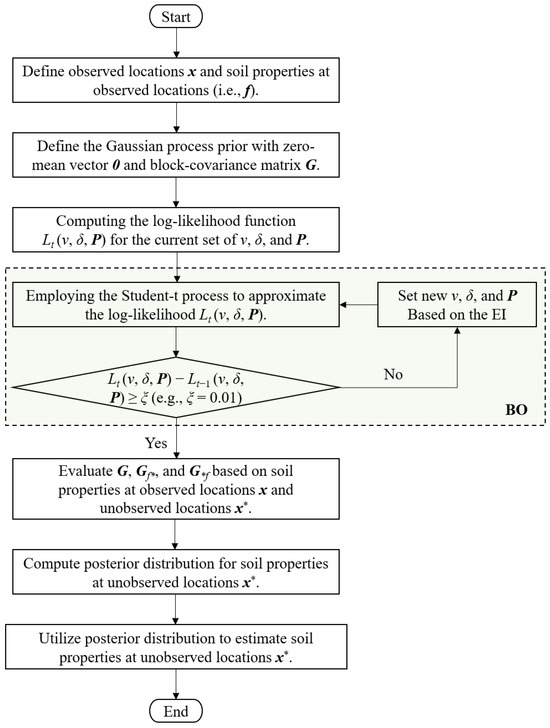
Figure 1.
Flowchart of the proposed BO-MOGP method for geotechnical site characterizations.
5. Case Study
5.1. A Synthetic Case
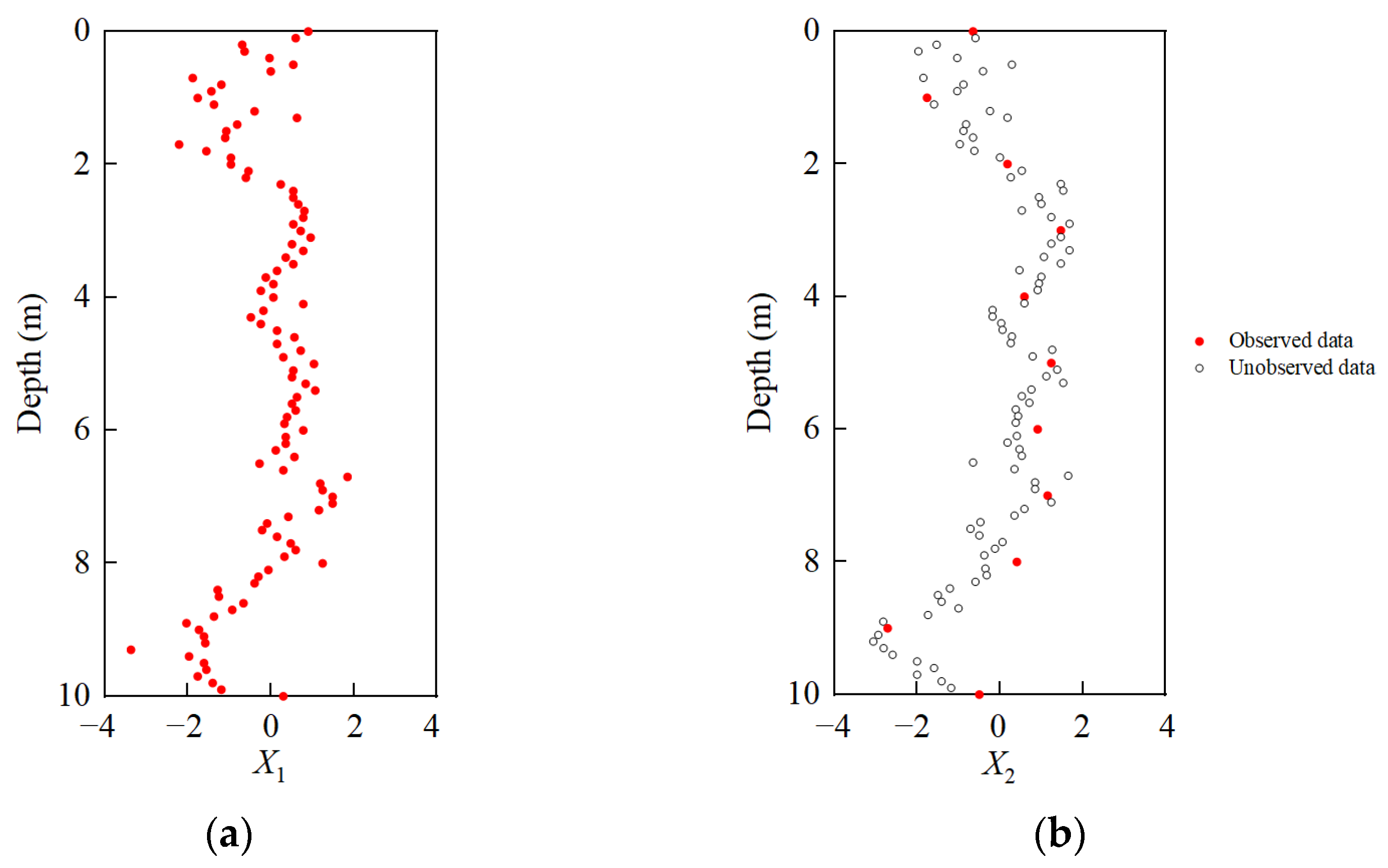
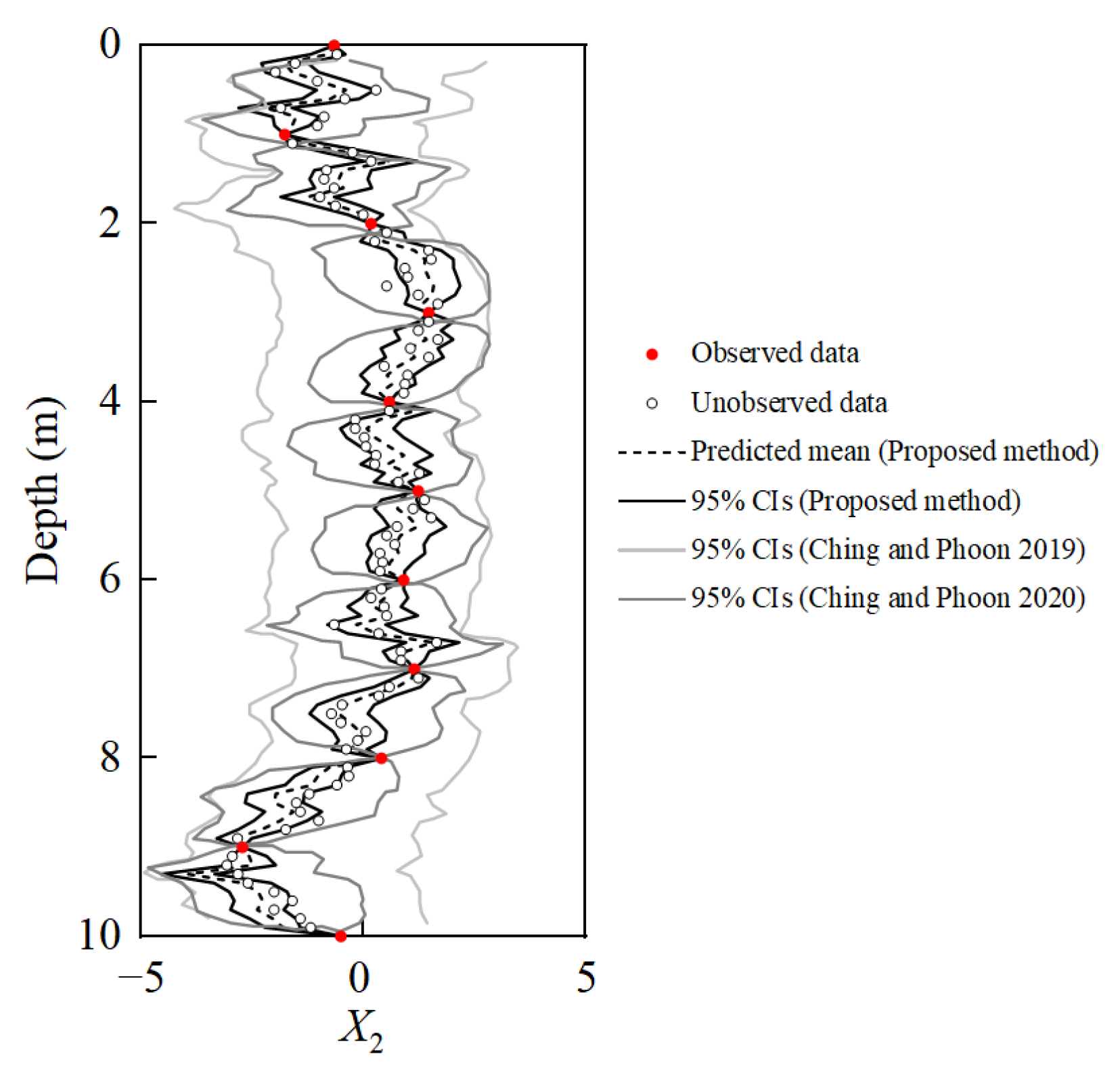
In this section, a detailed comparison is conducted between the work of Ching and Phoon [13] and the proposed method. The focus of this comparison is to evaluate the effectiveness of the approach in predicting soil properties using site-specific data. The data are bivariate, consisting of two variables, X1 and X2, which are correlated as indicated by the correlation matrix [1, 0.8; 0.8, 1]. These variables are modeled using the W-M model characterized by SOF = 1 m and ν = 0.5. The simulated data are shown in Figure 2. The simulated data for X1 are continuous, with a measurement interval of 0.1 m, making them abundant and providing a comprehensive view of the subsurface conditions. In contrast, X2 data are only available at 11 specific depths (0 m, 1 m, 2 m, …, 10 m). This sparse distribution of X2 data presents a challenge for accurate prediction at unobserved depths. The proposed model utilizes the available X1 and X2 data at observed locations to predict the X2 values at depths where they are not directly measured. The W-M model, with its specified SOF and ν values (SOF = 1.0 m, ν = 0.5), is employed within this framework. The predictions of X2 data are depicted in Figure 3. The uncertainty in the predictions made by the proposed BO-MOGP method is reduced compared to the earlier MUSIC method [12] and the MUSIC-X method [13]. This improvement is quantitatively evidenced by the narrower 95% confidence interval (CI) associated with the predictions. The enhanced performance of the proposed BO-MOGP method can be attributed to its ability to account for both spatial correlations among different depths and cross-correlations among different soil properties. This comprehensive consideration of correlations ensures a more accurate and reliable prediction of subsurface conditions. The predicted X2 profiles consistently pass through the 11 observed data points for X2, demonstrating the capability of the proposed BO-MOGP method to simulate a conditional random field, a feature that traditional MUSIC methods fail to incorporate. Further supporting the validity of the approach is the correlation matrix [1, 0.9; 0.9, 1] identified from the observed X1 and X2 data using the proposed BO-MOGP method. This matrix closely aligns with the actual correlation matrix, indicating that the proposed BO-MOGP method can effectively capture the true relationships among different soil properties. The proposed BO-MOGP model can utilize the cross-correlation between different soil properties even when the measurement locations are not the same. By using the cross-correlation structure, the model can transfer information between locations where different properties are measured, thereby enhancing prediction accuracy. This capability is particularly beneficial in sparse data scenarios.
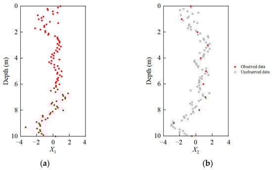
Figure 2.
Simulated data of (a) X1 and (b) X2.
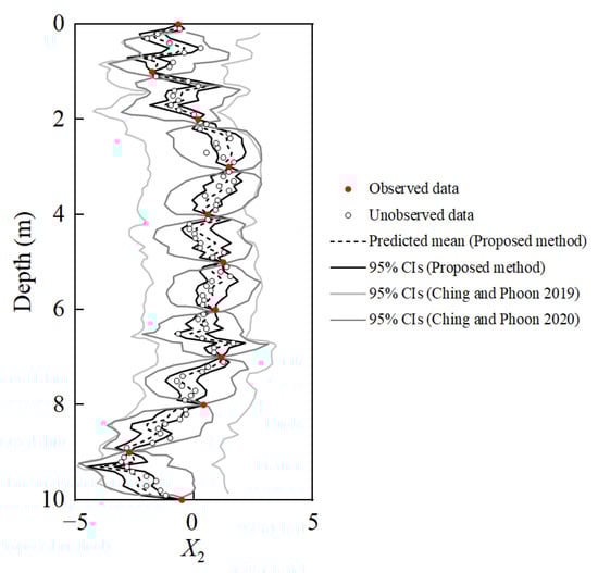
Figure 3.
The predicted mean values and 95% CIs of X2, together with results in [12,13].
5.2. A Real-World Case in Taipei
In the study of the silty clay layer at the Taipei site, a detailed examination is undertaken to analyze the spatial variability of the subsurface soil. This analysis focuses on seven soil properties including the liquid limit (LL), the plasticity index (PI), the liquidity index (LI), the vertical effective stress (σv′), the pre-consolidation stress (σp′), the undrained shear strength (Su), and the cone tip resistance (qt). Nondimensionalization is employed to normalize the dimensions of these soil properties, especially those inherently dimensional like σv′, σp′, Su, and qt. This method involves the use of natural logarithms to scale these soil properties against the atmospheric pressure (Pa = 101.3 kPa), a common reference point for pressure measurements in geotechnical engineering. Specifically, the transformations applied are as follows: σv′ and σp′ are rescaled to ln(σv′/Pa) and ln(σp′/Pa), respectively, to reflect variations in effective and pre-consolidation stresses normalized by atmospheric pressure; Su is converted to ln(Su/σv′), linking shear strength to effective stress in a dimensionless format; and qt is adjusted to ln[(qt − σv)/σv′], offering a normalized measure of cone resistance accounting for effective stress. These transformations yield a set of seven nondimensionalized variables: Y1 = LL, Y2 = PI, Y3 = LI, Y4 = ln(σv′/Pa), Y5 = ln(σp′/Pa), Y6 = ln(Su/σv′), and Y7 = ln[(qt − σv)/σv′]. In this study, detailed profiling is possible for Y4 and Y7 across a continuous depth interval of 0.1 m, ranging from 12.8 m to 26.6 m beneath the surface. This comprehensive data set provides a clear picture of the vertical effective stress and cone tip resistance variation with depth. In contrast, the parameters Y1, Y2, Y3, Y5, and Y6 are measured at discrete intervals, reflecting the practical limitations of soil sampling and testing. These discrete measurements are compiled in Table 1, presenting the depth-specific values for each parameter.

Table 1.
Site investigation results for the silty clay layer at the Taipei site.
The hyperparameters ν, δ, and P are estimated using Bayesian optimization, with ν = 0.5, and δ = 5.3, respectively. The P is shown in Table 2. The correlation matrix R can be derived through this matrix P and is shown in Table 3.
Table 2.
The identified covariance matrix P of the proposed BO-MOGP method.
Table 3.
The identified correlation matrix R of the proposed BO-MOGP method.
The rationality of the correlation matrix can be understood through the physical meaningfulness of the relationships among different soil properties. A positive correlation between the LL and PI is expected, as both are indicators of soil plasticity, with higher LL values typically corresponding to higher PI values. Conversely, a negative correlation is anticipated between the LI and qt1, as LI measures soil consistency, with higher values indicating a more liquid-like state, while qt1 measures soil strength, with higher values indicating stronger soil. Thus, soil with higher LI would generally have lower qt1. Additionally, a positive correlation might exist between the σp′ and Su, as both are related to soil strength, with higher σp′ often indicating that the soil has been subjected to greater loads in the past and may have higher Su. Furthermore, a positive correlation is expected between the σv′ and σp′, as both parameters are related to the stress history of the soil, with higher σv′ potentially leading to higher σp′ if the soil has been compressed and consolidated under the weight of overlying layers. These relationships ensure that the correlation matrix reflects the known behavior of the soil, providing a solid foundation for further analysis and modeling in geotechnical engineering.
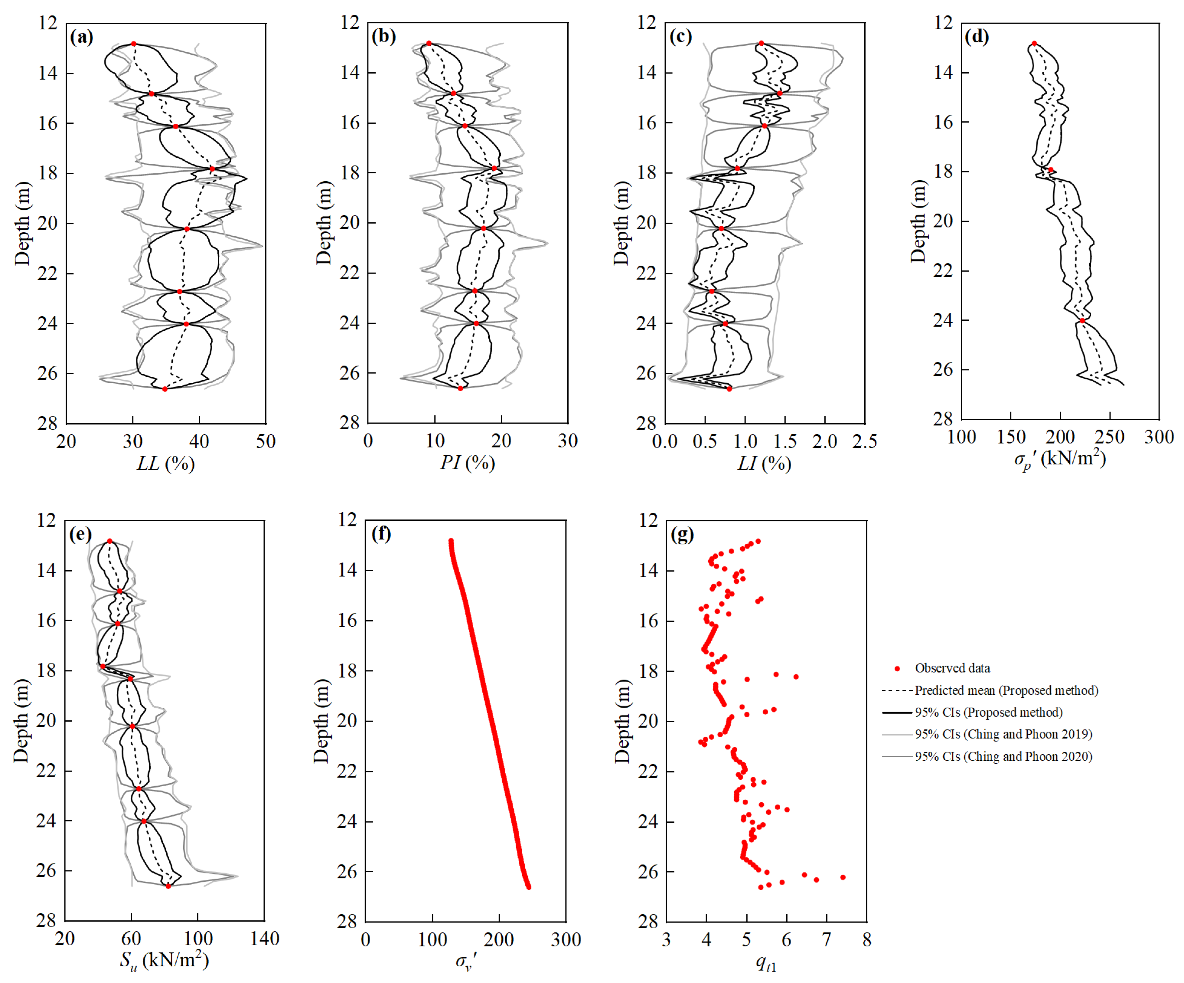
The estimations of soil properties using the proposed BO-MOGP method are shown in Figure 4. The 95% CI of each property is narrower than the MUSIC method and MUSIC-X method. The narrower confidence intervals indicate that the BO-MOGP method provides more precise and reliable predictions. This improvement in precision is particularly evident in instances of sparse data collection, such as the measurements of pre-consolidation stress (σp′) within the soil depth ranging from 12.8 m to 26.6 m. Despite having only three data points across this depth interval, the proposed BO-MOGP method demonstrates a remarkable reduction in the uncertainty of σp′ estimations, which, with traditional MUSIC and MUSIC-X methods, exhibit significant deviations from actual values, sometimes exceeding 105 kN/m3. The inability of the traditional MUSIC and MUSIC-X methods to account for the cross-correlations among different soil properties underlies these deviations. These methods are designed to handle sparse and incomplete data but fall short in using the interdependencies between soil properties. As a result, significant information that could improve prediction accuracy is not utilized, especially for parameters like σp′, which are measured infrequently. In contrast, the proposed BO-MOGP model incorporates both the spatial auto-correlations of individual soil properties and the cross-correlations among various soil properties. This dual-correlation feature allows the proposed BO-MOGP method to make use of the interdependencies among different soil properties, enhancing the accuracy of parameter estimations even in locations that have not been directly observed.
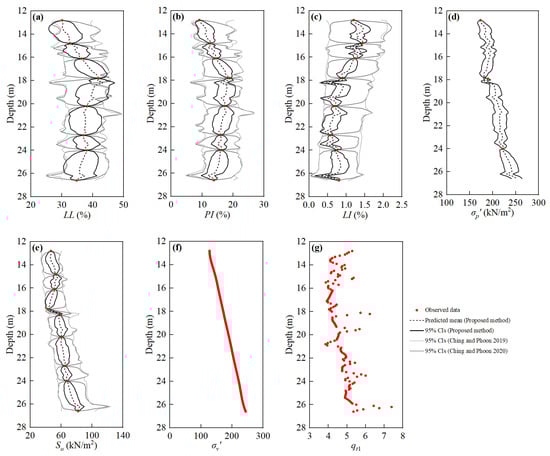
Figure 4.
Estimations of soil properties using the proposed BO-MOGP method: (a) LL; (b) PI; (c) LI; (d) σp′; (e) Su; (f) σv′; (g) qt1, comparing with Ching and Phoon [12,13].
6. Conclusions
This paper presents a novel DDSC method that utilizes the BO-MOGP to capture both the spatial correlations across different locations and the cross-correlations among various soil parameters. This dual-correlation feature enhances the accuracy of soil property predictions since it has the benefit of exploiting the soil properties’ correlations. The effectiveness of this method is demonstrated in a simulated example and a case study of Taipei. The conclusions are summarized below:
- The 95% CIs of the proposed BO-MOGP method for each soil property are narrower than those of traditional methods. This improvement is especially notable in scenarios with sparse data, as the proposed BO-MOGP method uses the interdependencies among different soil properties. This is because the proposed BO-MOGP method has the benefit of transferring information from measured soil properties to the soil properties in locations that have not been directly observed.
- The correlation matrix of soil properties derived from the site-specific data is accurately obtained by using the proposed BO-MOGP method. This indicates that the proposed method can effectively capture the true relationships among different soil properties.
- The proposed BO-MOGP method has the ability to generate conditional random field samples of multiple soil properties simultaneously, which is helpful in providing a comprehensive view of subsurface conditions. By offering a more accurate estimation of soil properties, the proposed BO-MOGP method can help reduce the uncertainty and risk associated with geotechnical engineering design, leading to a safe and reliable engineering solution.
Author Contributions
Conceptualization, H.X.; methodology, M.-Q.P. and H.X.; software, M.-Q.P. and Z.-C.Q.; validation, Y.-C.L. and J.-J.Z.; investigation, M.-Q.P. and Z.-C.Q.; data curation, M.-Q.P. and Z.-C.Q.; writing—original draft preparation, Z.-C.Q., Y.-C.L. and J.-J.Z.; writing—review and editing, M.-Q.P., S.-L.S. and H.X.; supervision, H.X.; funding acquisition, M.-Q.P., S.-L.S. and H.X. All authors have read and agreed to the published version of the manuscript.
Funding
This research was funded by the National Natural Science Foundation of China, Grant Nos. 42307200, 52108354, 42172309.
Institutional Review Board Statement
Not applicable.
Informed Consent Statement
Not applicable.
Data Availability Statement
The original contributions presented in the study are included in the article’s material; further inquiries can be directed to the corresponding author.
Conflicts of Interest
The authors declare no conflicts of interest.
References
- Chen, W.; Ding, J.; Wang, T.; Connolly, D.P.; Wan, X. Soil property recovery from incomplete in-situ geotechnical test data using a hybrid deep generative framework. Eng. Geol. 2023, 326, 107332. [Google Scholar] [CrossRef]
- Mitchell, J.K.; Soga, K. Fundamentals of Soil Behavior; John Wiley & Sons: New York, NY, USA, 2005. [Google Scholar]
- Liu, C.; Ji, F.; Song, Y.; Wang, H.; Li, J.; Xuan, Z.; Zhao, M. Upper bound analysis of ultimate pullout capacity for a single pile using Hoek–Brown failure criterion. Buildings 2023, 13, 2904. [Google Scholar] [CrossRef]
- Kostrzewa, J.; Popielski, P.; Dąbska, A. Geotechnical properties of washed mineral waste from grit chambers and its potential use as soil backfill and road embankment materials. Buildings 2024, 14, 766. [Google Scholar] [CrossRef]
- Bozzano, F.; Andreucci, A.; Gaeta, M.; Salucci, R. A geological model of the buried Tiber River valley beneath the historical centre of Rome. Bull. Eng. Geol. Environ. 2000, 59, 1–21. [Google Scholar] [CrossRef]
- Nowak, S.; Sherizadeh, T.; Esmaeelpour, M.; Brooks, P.; Guner, D.; Karadeniz, K. Numerical back analysis of an underground bulk mining operation using distributed optical fiber sensors for model calibration. Bull. Eng. Geol. Environ. 2024, 83, 71. [Google Scholar] [CrossRef]
- Phoon, K.-K.; Ching, J.; Shuku, T. Challenges in data-driven site characterization. Georisk Assess. Manag. Risk Eng. Syst. Geohazards 2022, 16, 114–126. [Google Scholar] [CrossRef]
- Cai, Y.; Phoon, K.K.; Pan, Q.; Luo, W. Modifying the Tailored Clustering Enabled Regionalization (TCER) framework for outlier site detection and inference efficiency. Eng. Geol. 2024, 335, 107537. [Google Scholar] [CrossRef]
- Mavritsakis, A.; Schweckendiek, T.; Teixeira, A.; Smyrniou, E.; Nuttall, J. Bayesian analysis of benchmark examples for data-driven site characterization. ASCE-ASME J. Risk Uncertain. Eng. Syst. Part A Civ. Eng. 2023, 9, 04023008. [Google Scholar] [CrossRef]
- Shuku, T.; Phoon, K.K. Comparison of data-driven site characterization methods through benchmarking: Methodological and application aspects. ASCE-ASME J. Risk Uncertain. Eng. Syst. Part A Civ. Eng. 2023, 9, 04023006. [Google Scholar] [CrossRef]
- Phoon, K.K.; Zhang, W. Future of machine learning in geotechnics. Georisk Assess. Manag. Risk Eng. Syst. Geohazards 2023, 17, 7–22. [Google Scholar] [CrossRef]
- Ching, J.; Phoon, K.-K. Constructing site-specific multivariate probability distribution model using Bayesian machine learning. J. Eng. Mech. 2019, 145, 04018126. [Google Scholar] [CrossRef]
- Ching, J.; Phoon, K.-K. Constructing a site-specific multivariate probability distribution using sparse, incomplete, and spatially variable (MUSIC-X) data. J. Eng. Mech. 2020, 146, 04020061. [Google Scholar] [CrossRef]
- Wang, Y.; Zhao, T. Interpretation of soil property profile from limited measurement data: A compressive sampling perspective. Can. Geotech. J. 2016, 53, 1547–1559. [Google Scholar] [CrossRef]
- Wang, Y.; Zhao, T. Statistical interpretation of soil property profiles from sparse data using Bayesian compressive sampling. Géotechnique 2017, 67, 523–536. [Google Scholar] [CrossRef]
- Wang, Y.; Zhao, T.; Phoon, K.K. Direct simulation of random field samples from sparsely measured geotechnical data with consideration of uncertainty in interpretation. Can. Geotech. J. 2018, 55, 862–880. [Google Scholar] [CrossRef]
- Yang, H.Q.; Zhang, L. Bayesian back analysis of unsaturated hydraulic parameters for rainfall-induced slope failure: A review. Earth-Sci. Rev. 2024, 251, 104714. [Google Scholar] [CrossRef]
- Rana, H.; Sivakumar Babu, G.L. Probabilistic back analysis for rainfall-induced slope failure using MLS-SVR and Bayesian analysis. Georisk Assess. Manag. Risk Eng. Syst. Geohazards 2024, 18, 107–120. [Google Scholar] [CrossRef]
- Sheil, B. Prediction of microtunnelling jacking forces using a probabilistic observational approach. Tunn. Undergr. Space Technol. 2021, 109, 103749. [Google Scholar] [CrossRef]
- Tang, L.; Na, S. Comparison of machine learning methods for ground settlement prediction with different tunneling datasets. J. Rock Mech. Geotech. Eng. 2021, 13, 1274–1289. [Google Scholar] [CrossRef]
- Xie, J.; Huang, J.; Zeng, C.; Huang, S.; Burton, G.J. A generic framework for geotechnical subsurface modeling with machine learning. J. Rock Mech. Geotech. Eng. 2022, 14, 1366–1379. [Google Scholar] [CrossRef]
- Yoshida, I.; Tomizawa, Y.; Otake, Y. Estimation of trend and random components of conditional random field using Gaussian process regression. Comput. Geotech. 2021, 136, 104179. [Google Scholar] [CrossRef]
- Rohmer, J.; Foerster, E. Global sensitivity analysis of large-scale numerical landslide models based on Gaussian-Process meta-modeling. Comput. Geosci. 2011, 37, 917–927. [Google Scholar] [CrossRef]
- Ching, J.; Phoon, K.K.; Yang, Z.; Stuedlein, A.W. Quasi-site-specific multivariate probability distribution model for sparse, incomplete, and three-dimensional spatially varying soil data. Georisk Assess. Manag. Risk Eng. Syst. Geohazards 2022, 16, 53–76. [Google Scholar] [CrossRef]
- Rahardjo, H.; Aung, K.K.; Leong, E.C.; Rezaur, R.B. Characteristics of residual soils in Singapore as formed by weathering. Eng. Geol. 2004, 73, 157–169. [Google Scholar] [CrossRef]
- Fredlund, D.G. Unsaturated soil mechanics in engineering practice. J. Geotech. Geoenviron. Eng. 2006, 132, 286–321. [Google Scholar] [CrossRef]
- Xu, J.; Yang, C. Probabilistic Back Analysis Based on Adam, Bayesian and Multi-output Gaussian Process for Deep Soft-Rock Tunnel. Rock Mech. Rock Eng. 2023, 56, 6843–6853. [Google Scholar] [CrossRef]
- Song, C.; Zhao, T.; Xu, L.; Huang, X. Probabilistic prediction of uniaxial compressive strength for rocks from sparse data using Bayesian Gaussian process regression with Synthetic Minority Oversampling Technique (SMOTE). Comput. Geotech. 2024, 165, 105850. [Google Scholar] [CrossRef]
- Wang, L.; Pan, Q.; Wang, S. Data-driven predictions of shield attitudes using Bayesian machine learning. Comput. Geotech. 2024, 166, 106002. [Google Scholar] [CrossRef]
- Zhao, T.; Song, C.; Lu, S.; Xu, L. Prediction of Uniaxial Compressive Strength Using Fully Bayesian Gaussian Process Regression (fB-GPR) with Model Class Selection. Rock Mech. Rock Eng. 2022, 55, 6301–6319. [Google Scholar] [CrossRef]
- Li, S.C.; He, P.; Li, L.P.; Shi, S.S.; Zhang, Q.Q.; Zhang, J.; Hu, J. Gaussian process model of water inflow prediction in tunnel construction and its engineering applications. Tunn. Undergr. Space Technol. 2017, 69, 155–161. [Google Scholar] [CrossRef]
- Lin, Q.; Hu, J.; Zhou, Q.; Cheng, Y.; Hu, Z.; Couckuyt, I.; Dhaene, T. Multi-output Gaussian process prediction for computationally expensive problems with multiple levels of fidelity. Knowl.-Based Syst. 2021, 227, 107151. [Google Scholar] [CrossRef]
- Atkinson, J.H. Non-linear soil stiffness in routine design. Géotechnique 2000, 50, 487–508. [Google Scholar] [CrossRef]
- Liu, H.; Cai, J.; Ong, Y.S. Remarks on multi-output Gaussian process regression. Knowl.-Based Syst. 2018, 144, 102–121. [Google Scholar] [CrossRef]
- Bonilla, E.V.; Williams, C.; Chai, K. Multi-task Gaussian process prediction. Adv. Neural Inf. Process. Syst. 2007, 20, 153–160. [Google Scholar]
- Williams, C.K.; Rasmussen, C.E. Gaussian Processes for Machine Learning; MIT Press: Cambridge, MA, USA, 2006. [Google Scholar]
Disclaimer/Publisher’s Note: The statements, opinions and data contained in all publications are solely those of the individual author(s) and contributor(s) and not of MDPI and/or the editor(s). MDPI and/or the editor(s) disclaim responsibility for any injury to people or property resulting from any ideas, methods, instructions or products referred to in the content. |
© 2024 by the authors. Licensee MDPI, Basel, Switzerland. This article is an open access article distributed under the terms and conditions of the Creative Commons Attribution (CC BY) license (https://creativecommons.org/licenses/by/4.0/).