Landscape Ecological Security of the Lijiang River Basin in China: Spatiotemporal Evolution and Pattern Optimization

Abstract

The ecological security of karst basins is receiving increased attention as a result of intense human activity and climate change. However, how ecological security evolves in spacetime and the optimization of ecological security patterns still remain unclear. This study developed a methodological framework for evaluating ecological security and optimizing ecological security patterns of the Lijiang River Basin (LRB). The 3S technology was used to analyze the current status and evolution characteristics of landscape ecological security in the LRB from 1990 to 2020. This study identified and optimized ecological security patterns by adhering to the basic paradigm of “source identification–resistance surface construction–corridor extraction–node determination”. The results showed that the overall ecological security of the LRB was at a medium to high level, with an index showing an initial increase followed by a decrease. The LRB exhibited 24 ecological pinch points, 74 ecological corridors, 30 ecological sources, and 6 ecological barrier points. The predominant landscape types found within these pinch points and barrier points encompass forests, cultivated land, and urban areas. A scheme of “three cores, two belts, and six zones” was proposed to optimize the ecological security pattern of the LRB. This study provides a theoretical basis and technical references for the integrated management of the rivers, grasslands, farmlands, mountains, lakes, forests, and sands in the LRB, as well as for the ecological restoration of other regions.

1. Introduction

Intense human activity and climate change have led to frequent extreme weather events, water scarcity, habitat fragmentation, and loss of ecological land, putting tremendous pressure on ecological systems [1]. How to maintain a balance between human development and ecosystem stability has become the main direction of recent research [2].

Ecological security is a critical component of national security, referring to the condition of an ecological environment within a given region that remains resilient and unharmed in the face of human or natural disturbances [3,4]. The level of ecological security in a region is indicative of the health and sustainability of its local ecosystems [5,6]. As a refined branch of ecological security, landscape ecological security pertains to the consistent provision of ecological services by diverse landscape types within a defined spatial and temporal framework [7]. China has taken many measures to build a firm national ecological security barrier. Current ecological security projects focused on areas with exceptional natural resources, strategic watersheds, and intricate ecosystems [2]. Watersheds play a vital role in the examination of landscape ecological security at a regional level, showcasing distinct regional attributes and spatial spillover effects [8]. However, there is a lack of effective ecological safety measures to cope with spatial development in the watershed.

The ecological security pattern, a prominent research focus in disciplines such as ecology and landscape studies, is a landscape ecological planning method utilized to delineate areas suitable for ecological restoration and biodiversity conservation [9], which refers to an ecological network formed by the interconnection of various ecosystems [10]. Currently, the prevailing and foundational approach for developing ecological security patterns is the “source identification–resistance surface construction–corridor extraction” paradigm [2,11,12]. Common methods for identifying ecological sources include Integrated Valuation of Ecosystem Services and Tradeoffs (INVEST) [13,14,15], morphological spatial pattern analysis (MSPA) [16], and land-use type assignment [17,18]. Resistance surface construction typically utilizes a comprehensive element type assignment method, which more effectively captures ecological spatial heterogeneity compared to single landscape type assignments [19]. The extraction of ecological corridors often involves techniques such as the least-cost path model [20,21,22], graph theory methods [23,24], and circuit theory [25,26]. In this study, based on the structural and functional characteristics of the candidate area, both the patch composition in the landscape space and its functional attributes were considered. In contrast to the conventional minimum cumulative resistance model, an ecological security model was developed using circuit theory to incorporate predicted species’ random migration paths and population diffusion probabilities, thereby integrating ecological and functional considerations of the landscape.

The LRB is recognized as a prominent tourist destination on a global scale and holds the distinction of being one of the earliest national 5A-level scenic areas in China. Situated within a characteristic karst landscape, the LRB is confronted with issues such as rocky desertification and the encroachment of cultivated land, posing obstacles to the socio-economic progress of the region. Consequently, the implementation of immediate actions is imperative to establish a comprehensive eco-environmental protection strategy encompassing the entire basin [27]. The proposal of the integrated management system, “mountains, rivers, forests, farmlands, lakes, grasslands, and sands” (MRFLCGS), is rooted in the macro perspective of ecological civilization. The components of the MRFLCGS system are interconnected as a cohesive ecological community, necessitating comprehensive measures for protection, restoration, and governance. Therefore, this study aims to develop a methodological framework for evaluating ecological security and optimizing ecological security patterns of the LRB. The specific objectives are to fulfill the following: (1) conduct a spatiotemporal evolution of landscape ecological security evaluation in the LRB; (2) identify the ecological security pattern from the aspects of ecological sources, resistance surfaces, and corridors; and (3) optimize the ecological security pattern of the LRB. The research results will contribute to achieving harmonious coexistence of humans and nature and protecting biodiversity. Furthermore, it can provide theoretical and technical references for the integrated ecological restoration and management of the MRFLCGS system.

2. Materials and Methods

2.1. Study Area

The LRB is located in the southwestern part of the Nanling Mountain Range, Guilin City, Guangxi Zhuang Autonomous Region, China. The LRBspans from geographic coordinates 24°18′ N to 25°41′ N and from 109°45′ E to 110°40′ E, and is part of the Pearl River system, originating from Mao’er Mountain in Xing’an County (Figure 1) [28]. The LRB encompasses six major urban areas including Guilin City, as well as counties such as Lingchuan, Yangshuo, Xing’an, and Pingle. With a total area of approximately 5837.95 km² and a main stream length of 164 km, the terrain of the basin gradually slopes from north to south and features granite mountains, karst landforms, semi-plains, and river valley basins. The LRB is characterized by a subtropical monsoon climate, with an annual precipitation range of 1400 to 2000 mm and red soil as the predominant soil type [29]. As one of the earliest tourism areas in China, the LRB possesses abundant tourism resources and a well-developed tourism industry, attracting a total of 102.41 million visitors and generating a tourism revenue of 123.354 billion yuan in Guilin City in 2020.

2.2. Data Sources

The remote sensing data utilized in this research were obtained from the Geographic Spatial Data Cloud website (http://www.gscloud.cn/, accessed on 23 December 2021). The study period was chosen to encompass September and October, months characterized by consistent plant growth and water level fluctuations. Following an analysis of vegetation growth trends and annual precipitation patterns in the LRB, four sets of remote sensing imagery data were ultimately chosen, i.e., October 1990 (Landsat 5 TM), September 2000 (Landsat 5 TM), October 2010 (Landsat 5 TM), and October 2020 (Landsat 8 OLI). The images provided valuable information regarding six distinct landscape types, including cultivated land, forest land, construction land, water bodies, grassland, and unused land. Furthermore, data pertaining to nighttime light levels were sourced from the Chinese Academy of Sciences’ Earth Noctilucent Dataset, also known as the Flint dataset. The calculation of the Normalized Difference Vegetation Index (NDVI) was conducted using ENVI 5.2 software on preprocessed remote sensing imagery data from 2020.

2.3. Research Framework

This study developed a methodological framework for assessing ecological security and optimizing ecological security patterns in the LRB (Figure 2). The framework consisted of three steps. In step 1, this study acquired data related to the thesis on land use, precipitation, statistics, etc. and performed data preprocessing. In step 2, this study demonstrated the current status and spatiotemporal evolution characteristics of landscape ecological security from 1990 to 2020. In step 3, this study constructed ecological security patterns by adhering to the basic paradigm of “source identification–resistance surface construction–corridor extraction–node determination”. Based on the current status and pattern of ecological security in the basin, optimization recommendations were proposed.

2.4. Landscape Ecological Security Evaluation Model

The landscape pattern index reflects both the internal structure and external spatial characteristics of the study area, providing valuable insights into the ecological environment status of the region [30]. Evaluation units are variable and related to the study objectives and the size of the study area [31,32]. Referring to related studies [33] and combining with the actual situation of the study area, the paper selects 1.5 km grid cells as the evaluation units. Various indicators, such as degree of breakage, degree of separation, ecological risk index, and landscape security index, were utilized to study the ecological security level of the LRB (

Table 1. Calculation method of landscape ecological security indices.

Indices name	Calculation Formula	Parameter Meaning
Degree of breakage	$C_i=N_i/A_i$	$N_i$ and $A_i$ represent the number and area of landscape-type patches, respectively.
Degree of separation	$$\begin{gathered} F_i=\sqrt{S_i}/2P_i \\ {S}_i=N_i/A \\ {P}_i=A_i/A \end{gathered}$$	$S_i\mathrm{a}\mathrm{n}\mathrm{d}{P}_i$ respectively represent the distance index and relative coverage of landscape types, and $A$ represents the total landscape area.
Dominance degree	$D_i={dL}_i+{eP}_i$	$L_i$ represents the relative density of landscape types. According to the actual situation of the study area, d and e are assigned with analytic hierarchy process (AHP), $d$ = 0.6, $e$ = 0.4.
Interference degree	$E_i=a{C}_i+b{F}_i+c{D}_i$	$C_i$, $F_i$ and $D_i$ respectively represent degree of fragmentation, degree of separation, and degree of dominance. According to the actual situation of the study area, a, b, and c are assigned by AHP, $a$ = 0.5, $b$ = 0.3, $c$ = 0.2.
Vulnerability	Cultivated land 0.2857, unutilized 0.2381, meadow 0.1905, Water body 0.1429, Forest land 0.0952, Construction land 0.0476	Assign values to each landscape type: cultivated land is 6, unused land is 5, grassland is 4, water body is 3, forest land is 2, and construction land is 1. After assigning values, normalization is processed.
Loss degree	$R_i=E_i\times V_i$	$E_i$ represents landscape disturbance index, $V_i$ represents vulnerability index (same as the former vulnerability index).
Ecological risk index	$LERI=\sum _{i=1}^N\frac{A_{ki}}{A_k}{W}_i$	$A_k$ is the total area of the k sample plot, $A_{ki}$ is the total area of landscape type of the k sample plot,$W_i$ is the category i ecological risk intensity parameter of AHP: forest land 0.0427, cultivated land 0.1916, construction land 0.3934, water body 0.1425, grassland 0.0726, and unused land 0.1572.
Ecological security index	$LESI=1/LERI$	$LESI$ stands for landscape ecological security index.

).

2.5. Spatial Autocorrelation Analysis

Spatial autocorrelation analysis is utilized to assess the level of similarity or correlation of a variable among spatial units within a specific geographic area, which helps to examine the extent of interaction among research subjects at the spatial scale [34]. In this research, both local spatial autocorrelation (LISA) and global spatial autocorrelation (Moran’s I) were utilized to examine the spatial metrics of landscape ecological security in the LRB.

(1)

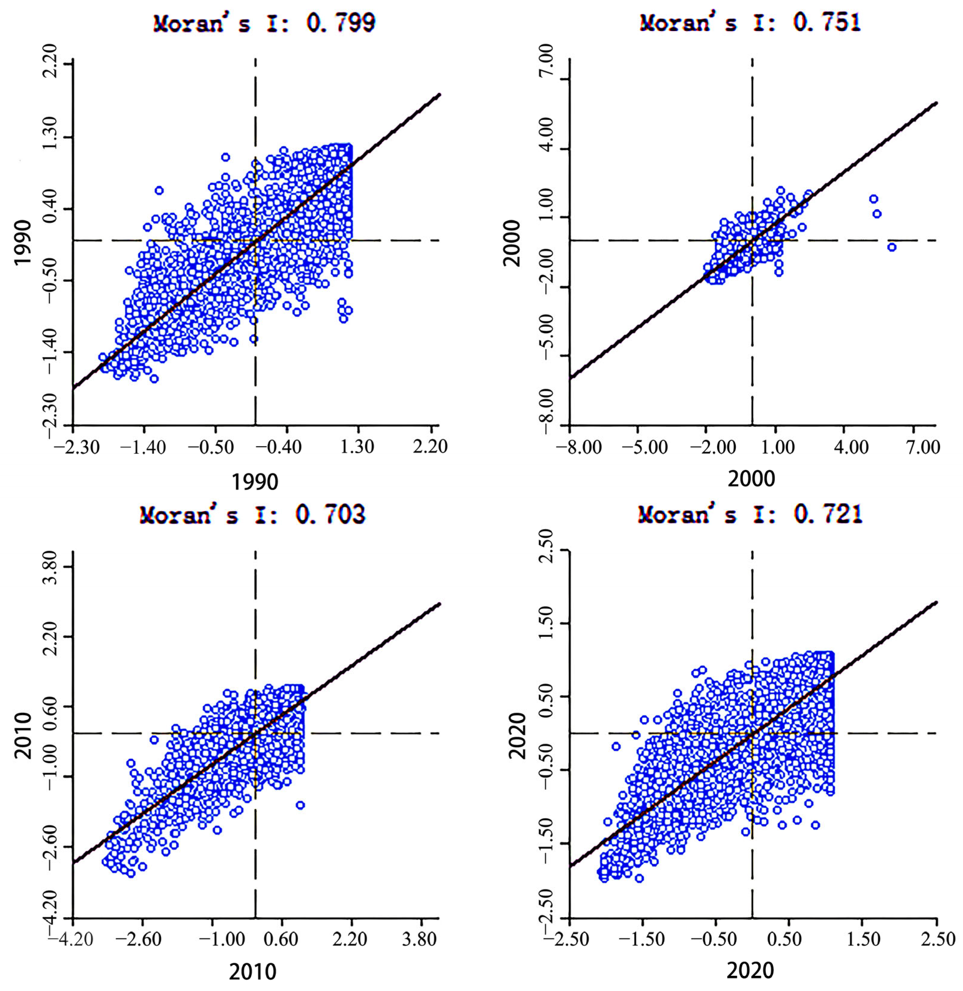
Global Spatial Autocorrelation (Moran’s I): It refers to the distribution characteristics of unit features across the entire space [35]. The formula for Moran’s I index is as follows:

$$\frac{{\sum }_{i=1}^n{\sum }_{j=1}^n{W}_{ij}\left(X_i-X_0\right)\left(X_j-X_0\right)}{S^2{\sum }_{i=1}^n{\sum }_{j=1}^n{W}_{ij}}$$

(1)

where I represents the global spatial autocorrelation index; $S^2$ is the sample variance; $W_{ij}$ means the spatial weight matrix; n means total number of regions; $X_i$ is the observed value of region i; and $X_0$ is the sample mean.

(2)

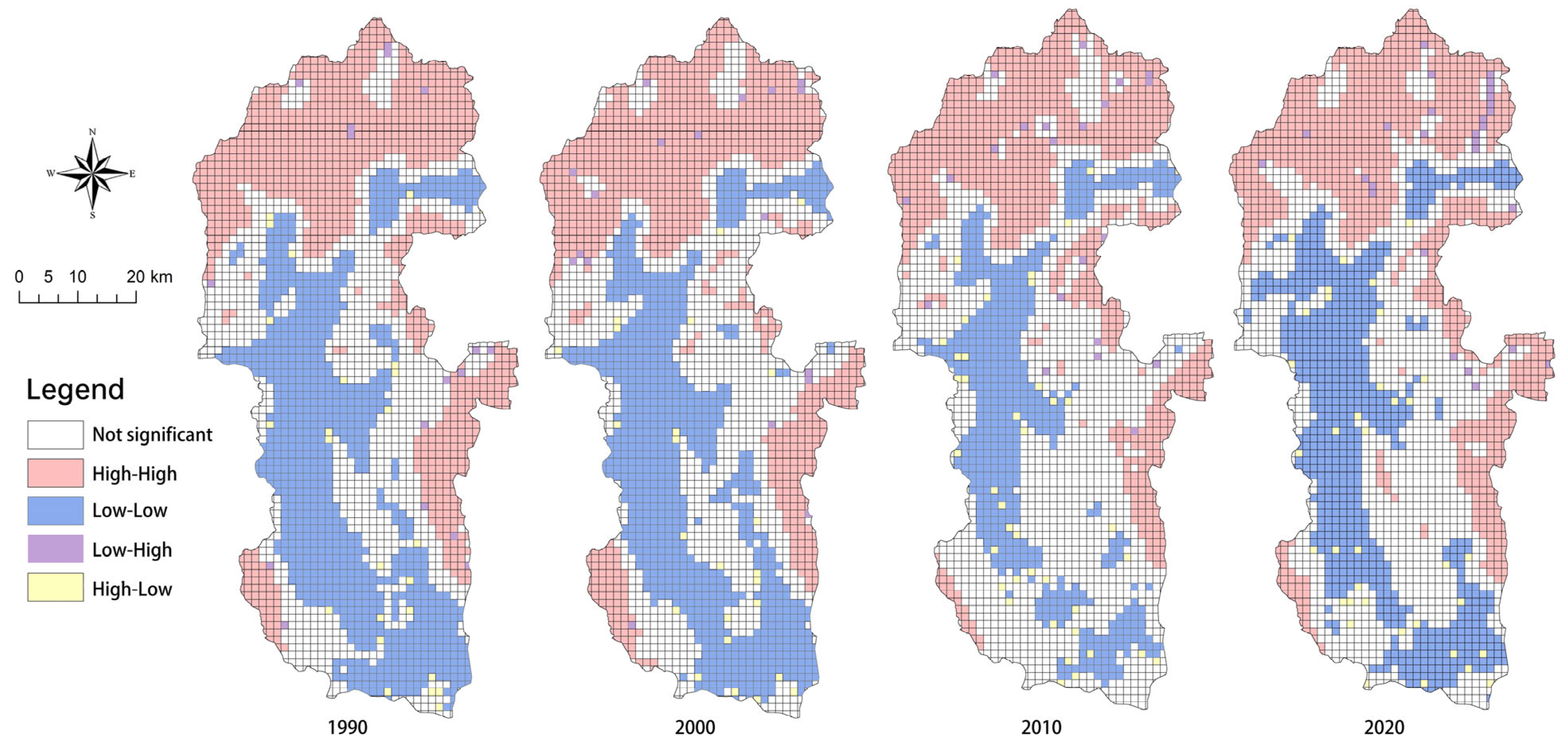
LISA: Local spatial autocorrelation refers to the spatial clustering or dispersion characteristics of spatial features within a local range [36]. The formula for calculating the LISA index is as follows:

$$I=\frac{\left(X_i-X_0\right)}{S^2}\sum _{j=1}^n{W}_{ij}\left(X_j-X_0\right)$$

(2)

where $I$ represents the LISA index; $S^2$ is the sample variance; $W_{ij}$ means the spatial weight matrix; $n$ means the total number of regions; $X_i$ is the observed value of region $i$; and $X_0$ is the sample mean.

2.6. Ecological Security Pattern Model

2.6.1. Identification of Ecological Sources

MSPA was used to detect the spatial configurations of the study area, effectively identifying landscape types and structures [37]. Utilizing the Guidos Tool Box 3.1 software, an eight-neighbor analysis approach was utilized to identify and classify seven distinct landscape types within the LRB, encompassing core areas, edge areas, connecting bridges, isolated patches, ring areas, gaps, and branches.

The InVEST model, developed by esteemed institutions such as Stanford University in the United States, is a freely accessible open-source tool. Specifically, the model’s Habitat Quality module enables the assessment of habitat quality based on the identified landscape types [38]. A habitat quality index closer to 1 signifies superior habitat quality, with the index typically ranging between 0 and 1. The study set up the model parameters with reference to the InVEST model manual and the actual conditions in the study area (

Table 2. Sensitivity of different landscape types to stress factors.

Landscape Types	Habitat Suitability $\left({\mathit{Q}}_{\mathit{x}\mathit{j}}\right)$	$\mathbf{Stress}\mathbf{Factors}({\mathit{D}}_{\mathit{x}\mathit{j}}$)
		Cultivated Land	Construction Land	Unutilized
Forest land	1.0	0.6	0.4	0.2
Cultivated land	0.1	0.2	0.8	0.5
Construction land	0.0	0.0	0.0	0.0
Water body	0.7	0.3	0.3	0.2
meadow	0.8	0.8	0.6	0.5
unutilized	0.4	0.5	0.4	0.2

).

$$Q_{xj}=H_j\left[1-\left(\frac{D_{2xj}}{D_{2xj+K^2}}\right)\right]$$

(3)

where $Q_{xj}$ represents the habitat quality of grid x in landscape utilization type $j$; $D_{xj}$ represents the level of habitat stress in landscape utilization type $j$ for grid $x$; $H_j$ represents the habitat suitability of landscape utilization type $j$; and $K$ represents the half-saturation constant.

This study extracted the core areas from the MSPA analysis results and then assigned weights and overlaid the analysis based on the results of habitat quality analysis (

Table 3. Superimposed weight assignment table of MSPA and InVEST model analysis results.

Types	Weight (%)	Reclassification Name	Reclassification Grade
MSPA analysis results	40	Core	1
		Islet	2
		Perforation	3
		Edge	3
		Bridge	2
		Loop	2
		Branch	3
Results of habitat quality analysis	60	High habitat quality areas (0.82–1.00)	1
		Medium habitat quality area (0.30–0.82)	2
		Low habitat quality area (0.00–0.30)	3

). Finally, patches with an area greater than 10 km² were identified as ecological sources. Landscape connectivity is defined as the degree to which ecological processes move between source patches and can reveal the organic connections between landscape elements [39]. Using Conefor 2.6 software with a distance of 2500 m and a connectivity probability of 0.5, the landscape connectivity of ecological sources was analyzed, and the patch importance index dPC was selected to rank the importance of ecological sources.

2.6.2. Construction of Ecological Resistance Surface

The scientific construction of ecological resistance factors holds considerable importance for biodiversity conservation efforts [40]. Based on the actual conditions of the LRB, elevation, slope, NDVI, landscape types, MSPA analysis results, habitat quality analysis results, and regional ecological security level were considered as resistance factors. The factors were categorized into five levels, and their weights were determined using the analytic hierarchy process (AHP) to create the resistance surface. In light of the influence of human activities on species diversity, raster nighttime light data reflecting the degree of human disturbance were employed. The average nighttime light value was computed by dividing the nighttime light data by the area of each landscape type, serving as the light parameter in the research area (Figure 3). Subsequently, this value was multiplied by the comprehensive resistance value to refine the ecological resistance surface.

2.6.3. Extraction of Ecological Corridors

Ecological corridors function as conduits linking source areas of ecological significance, facilitating species migration and providing essential ecological services, including the preservation of biodiversity and the facilitation of biological flows [41]. Circuit theory utilizes the characteristics of random electronic wandering in circuits to simulate the process of biological migration and diffusion [42]. In ArcCatalog 10.7, the Build Network and Map Linkages tool was employed in conjunction with the specific conditions of the study area to delineate a linear ecological corridor with a width of 2000 m. The formula is as follows:

$$I=V/R_{eff}$$

(4)

In the formula, $I$ represents the electric current in the conductor, $V$ represents the voltage across the conductor, and $R_{eff}$ means the effective resistance of the conductor. In ecology, $I$ is considered to reflect the process of biological migration movement, $V$ is considered the basis for selecting potential connectivity indices, and $R_{eff}$ is regarded as the impedance encountered in the process of biological migration movement.

2.6.4. Determination of Ecological Nodes

Ecological nodes are located in high-density current areas and represent regions that species may pass through or must pass through during the process of migration and diffusion, thereby reflecting landscape connectivity functions [43]. These nodes are vulnerable to ecological risks and instability when disrupted. The Pinchpoint Mapper function in ArcCatalog 10.7 was employed to pinpoint ecological nodes within the LRB. Ecological barriers, on the other hand, denote regions where species encounter substantial obstacles during migration and diffusion from ecological sources [44]. The Barrier Mapper function was employed to recognize ecological barrier points.

3. Results

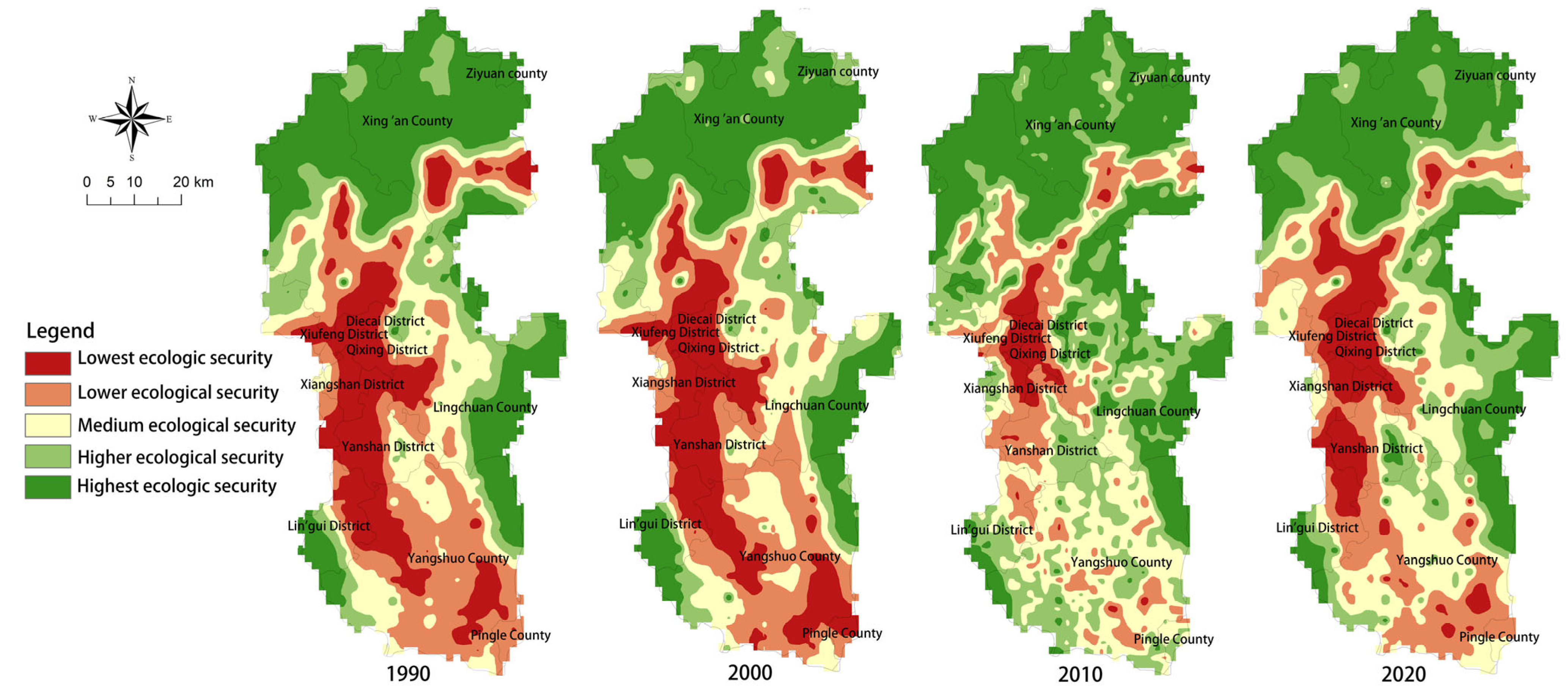
3.1. Spatiotemporal Evolution of Landscape Ecological Security

The area and number of patches for each landscape type were extracted for each year in Fragstats 4.2 software. Subsequently, fragmentation, isolation, dominance, disturbance, fragility, loss, ecological risk index, and ecological security index (LESI) were calculated for the LRB in 1990, 2000, 2010, and 2020 according to specific formulas (

Table 4. Landscape type area and landscape ecological security indices of the LRB from 1990 to 2020.

Landscape Types	Time	Area/km2	${\mathit{C}}_{\mathit{i}}$	${\mathit{F}}_{\mathit{i}}$	${\mathit{D}}_{\mathit{i}}$	${\mathit{E}}_{\mathit{i}}$	${\mathit{V}}_{\mathit{i}}$	${\mathit{R}}_{\mathit{i}}$	$\mathbf{L}\mathbf{E}\mathbf{R}\mathbf{I}$	$\mathbf{L}\mathbf{E}\mathbf{S}\mathbf{I}$
Forest land	1990	4178.946	0.023	0.054	0.438	0.115	0.095	0.011	0.083	11.985
	2000	4334.957	0.014	0.043	0.407	0.101	0.095	0.010	0.081	12.348
	2010	4528.033	0.006	0.030	0.405	0.093	0.095	0.009	0.078	12.879
	2020	4633.304	0.005	0.028	0.433	0.098	0.095	0.009	0.083	12.112
Cultivated land	1990	1284.440	0.092	0.033	0.277	0.112	0.286	0.032	0.083	11.985
	2000	1102.731	0.075	0.026	0.230	0.091	0.286	0.026	0.081	12.348
	2010	835.191	0.026	0.012	0.134	0.043	0.286	0.012	0.078	12.879
	2020	554.331	0.045	0.010	0.164	0.059	0.286	0.017	0.083	12.112
Construction land	1990	82.634	0.180	0.003	0.029	0.097	0.048	0.005	0.083	11.985
	2000	119.303	0.264	0.005	0.067	0.147	0.048	0.007	0.081	12.348
	2010	176.450	0.060	0.004	0.049	0.041	0.048	0.002	0.078	12.879
	2020	379.746	0.062	0.008	0.145	0.062	0.048	0.003	0.083	12.112
Water body	1990	111.572	0.233	0.005	0.049	0.128	0.143	0.018	0.083	11.985
	2000	110.624	0.157	0.004	0.040	0.087	0.143	0.012	0.081	12.348
	2010	105.980	0.040	0.002	0.022	0.025	0.143	0.004	0.078	12.879
	2020	110.628	0.032	0.002	0.025	0.022	0.143	0.003	0.083	12.112
Meadow	1990	167.676	0.710	0.012	0.201	0.399	0.191	0.076	0.083	11.985
	2000	154.727	0.778	0.012	0.235	0.440	0.191	0.084	0.081	12.348
	2010	174.998	0.601	0.012	0.380	0.380	0.191	0.072	0.078	12.879
	2020	146.009	0.283	0.007	0.217	0.187	0.191	0.036	0.083	12.112
Unutilized	1990	12.700	0.208	0.000	0.005	0.105	0.238	0.025	0.083	11.985
	2000	15.587	0.164	0.001	0.006	0.083	0.238	0.020	0.081	12.348
	2010	17.278	0.155	0.001	0.011	0.080	0.238	0.019	0.078	12.879
	2020	13.952	0.201	0.001	0.015	0.104	0.238	0.025	0.083	12.112

). Analysis of the ecological security index revealed that the landscape ecological security of each landscape type fluctuated within the range of 11.985 to 12.879 from 1990 to 2020. The overall trend of ecological security over the past thirty years of the ecological security index exhibited an inverted “V” shape, with an initial increase followed by a decrease. Specifically, the ecological security index rose from 11.985 in 1990 to 12.879 in 2010 and then decreased to 12.112.

Spatial distribution of landscape ecological security in the LRB from 1990 to 2020 was obtained using Kriging interpolation and clustered into five levels by the natural breakpoints method (Figure 4). From a spatial analysis, it could be observed that regions exhibiting high and moderately high levels of ecological security were concentrated in the northern and southeastern portions of the study area, notably in Lingchuan County and Xing’an County, characterized by extensive forest coverage. In contrast, areas with moderately low and low ecological security were predominantly situated in the central and southern regions of the study area, specifically in Diecai District, Xiufeng District, and Qixing District, where construction and cultivated land were prevalent.

Regarding the ecological security level of landscape patterns in the study area over the years, it can be observed that the overall ecological security status in the LRB from 1990 to 2020 remained at a moderately high level. As shown in

Table 5. Area and proportion of landscape ecological security level in the LRB from 1990 to 2020.

Ecological Security Level	1990		2000		2010		2020
	Area (km2)	Proportion (%)	Area (km2)	Proportion (%)	Area (km2)	Proportion (%)	Area (km2)	Proportion (%)
Highest ecological security	1869.75	32.02	1737	29.75	2214	37.92	1917	32.83
Higher ecological security	812.25	13.91	832.50	14.26	1377	23.58	967.50	16.57
Medium ecological security	949.50	16.26	1046.25	17.92	1262.25	21.62	1210.50	20.73
Lower ecological security	1212.75	20.77	1143	19.58	774	13.26	1111.50	19.04
Lowest ecological security	994.50	17.03	1080	18.50	211.50	3.62	632.25	10.83

, overall, the areas of lowest and lower ecological security showed a decreasing trend over time, whereas the areas of highest and higher ecological security exhibited an increasing trend. In the past thirty years, the area of lowest ecological security decreased the most, with a significant reduction of 362.25 km², while the area of medium ecological security increased the most, with a substantial increment of 261 km². The area of the highest ecological security has consistently remained dominant, and their proportion has increased each year, reaching a proportion as high as 37.92% in 2010. On the other hand, the area of lowest ecological security has gradually decreased and accounted for a relatively small proportion, with only 3.62% in 2010.

The areas of landscape ecological security in 1990 and 2020 were analyzed using a raster calculator, resulting in the landscape type area transition matrix for the LRB (1990–2020) (

Table 6. Area transition matrix of landscape ecological security from 1990 to 2000 (subsection).

	2020	Highest Ecological Security	Higher Ecological Security	Medium Ecological Security	Lower Ecological Security	Lowest Ecological Security
1990
Highest ecological security		519.75	445.50	0.00	0.00	0.00
Conversion rate		—	46.15%	0.00%	0.00%	0.00%
Higher ecological security		112.50	515.25	537.75	45.00	0.00
Conversion rate		9.29%	—	44.42%	3.72%	0.00%
Medium ecological security		0.00	101.25	528.75	292.5	27.00
Conversion rate		0.00%	10.66%	—	30.81%	2.84%
Lower ecological security		0.00	0.00	110.25	461.25	191.25
Conversion rate		0.00%	0.00%	14.45%	—	25.07%
Lowest ecological security		0.00	0.00	6.75	166.50	1696.50
Conversion rate		0.00%	0.00%	0.36%	8.90%	—

). Among them, the changes in highest, higher, and medium ecological security were the most significant. Highest ecological security mainly transformed into higher ecological security, with a conversion rate of 46.15%. Higher ecological security primarily transformed into highest ecological security and medium ecological security, with conversion rates of 9.29% and 44.42%, respectively.

3.2. Spatial Autocorrelation of Landscape Ecological Security Index

GeoDa 1.18 software was utilized to examine the spatial distribution pattern of the ecological security index in the LRB (Figure 5). The index values showed a decreasing-then-increasing trend. The global Moran’s I estimated for the years 1990, 2000, 2010, and 2020 were 0.799, 0.751, 0.703, and 0.721, respectively, indicating that the ecological security index in the LRB did not exhibit a random distribution. Instead, it displayed positive spatial autocorrelation, demonstrating a high degree of similarity and clustered distribution.

Based on the results of LISA analysis (Figure 6), the low–low and high–high clusters of the landscape ecological security index in each period were distinct and exhibited a lower level of aggregation, indicating a high similarity in their distribution. The high–high clusters were mainly concentrated in the northern and eastern areas of the LRB, characterized by forested areas with low landscape fragmentation, good habitat quality, and minimal human disturbance. The low–low clusters were primarily concentrated in urban areas along the Lijiang River, such as the central area of Lingchuan County, Xing’an County, Guilin, and other regions. These parts were predominantly composed of construction land, had a high degree of economic development, numerous tourist attractions, and significant human activities.

3.3. Construction and Optimization of Landscape Ecological Patterns

3.3.1. Identification of Ecological Sources Based on the MSPA and InVEST Model

The Reclassify tool was utilized to assign a value of 1 to the forest landscape type, with other landscape types receiving a value of 0. Subsequently, a raster binary map was generated, facilitating the acquisition of MSPA classification results for landscape types within the LRB. The InVEST model was utilized to analyze the habitat quality index in the LRB, and the results were categorized into five classes by the natural breakpoints approach (Figure 7). The core area of the LRB covered approximately 4194.26 km², constituting 71.84% of the overall study area. This core area was predominantly situated in the eastern region of Xing’an County, the northern region of Lingchuan County, and Yangshuo County, encompassing 90.52% of the total forested area. Yangshuo County (873.15 km²) and Xing’an County (1069.22 km²) have the largest core area, accounting for 30.07% and 36.82% of the total core area, respectively.

Regions with high and moderately high habitat quality were predominantly concentrated in the eastern and northern regions of the study area, particularly in Lingchuan County, Xing’an County, and Yangshuo County (Figure 7). These areas covered approximately 4779.03 km², accounting for 81.86% of the total study area. The spatial distribution of these regions closely aligned with the results of the MSPA landscape type analysis and the distribution of forested areas. Conversely, regions with low habitat quality were predominantly located in the central part of the study area, corresponding to urban areas with high levels of human activity (Figure 7). These regions were mainly distributed in Lingchuan County and Yangshuo County, covering approximately 934.32 km², which accounted for 16.00% of the total study area. In summary, the overall habitat quality in the LRB was good, with a tendency towards polarization. Areas of high habitat quality were mainly distributed in areas with sparse people and abundant vegetation, while areas of low habitat quality were mainly located in areas with frequent human activities and a developed economy.

3.3.2. Identification of Ecological Sources

This study used high habitat quality areas to correct the core area and then performed the weight assignment of both and superimposed analysis. Finally, the patches with an area of more than 10 km² were extracted as ecological sources (Figure 8). The total area of the patches was 3960.08 km², which accounted for 67.83% of the total area of the study area and was mainly distributed in Lingchuan, Xing’an, and Yangshuo Counties. The ecological sources in the LRB were ranked from high to low according to the dPC in Conefor 2.6 software. Seven of the patches with high dPC values were selected as core ecological sources (dPC > 10), and the remaining 23 patches were general ecological sources (dPC ≤ 10) (

Table 7. Ecological source connectivity indices.

Grade	Plaque Numbering	Area/km2	Account for the Proportion of the Study Area/%	Patch Significance Index (dpc)
Core ecological source	7	1150.80	19.71%	59.69
	15	686.59	11.76%	57.28
	23	592.41	10.15%	35.20
	21	263.61	4.52%	15.80
	28	288.21	4.94%	13.23
	2	27.71	0.47%	12.59
	3	12.96	0.22%	11.96
General ecological source	10	193.96	3.32%	9.55
	6	104.96	1.80%	5.43
	5	10.15	0.17%	5.16
	9	92.26	1.58%	4.72
	14	78.33	1.34%	4.03
	1	59.43	1.02%	2.99
	4	30.81	0.53%	2.80
	20	26.91	0.46%	1.57
	8	31.88	0.55%	1.55
	29	25.09	0.43%	1.54
	17	56.48	0.97%	1.45
	11	26.24	0.45%	1.43
	19	27.19	0.47%	1.34
	27	26.08	0.45%	1.24
	24	22.50	0.39%	1.12
	16	17.87	0.31%	1.03
	30	21.45	0.37%	1.02
	22	15.43	0.26%	0.87

).

3.3.3. Construction of Ecological Resistance Surface

The comprehensive resistance surface was calculated by weighting the superposition of the resistance factors, followed by the application of lighting parameters to adjust the surface. The resulting modified resistance surface was then visualized in a grid diagram (Figure 9). The areas with high resistance values were predominantly located in low ecological security regions, such as the central urban area, while areas with low resistance values were primarily found in the highest ecological security regions, such as forest land.

3.3.4. Extraction of Ecological Corridors

The distribution map of ecological corridors in the LRB was generated using circuit theory based on identified ecological sources and a modified resistance surface (Figure 10). Two categories of ecological corridors—key ecological corridors and potential ecological corridors—were identified in the study area. There were 58 key ecological corridors with a total length of about 179.77 km and an average length of 3.1 km, which were mainly located in the northern and eastern parts of Lingchuan County, the southern part of Yangshuo County, the eastern part of Xing’an County, and the northern part of Yanshan District. There were 16 potential ecological corridors with a total length of about 140.66 km and an average length of 8.79 km, which were mainly located in the western part of Lingchuan County, the southern part of Yangshuo County, the eastern part of Lingui District, and the southern part of Xiangshan District. There were 12 key corridors and 7 potential corridors that cross at least two administrative districts. The main landscape types under the ecological corridors are forests, cultivated land, construction land, and water bodies.

3.3.5. Determination of Ecological Nodes

A 1.5 km cost-weighted corridor width was set to construct a map of cumulative current values and location distribution of ecological nodes (Figure 11). There were 24 significant ecological nodes (cumulative current > 0.50) in the study area, covering an area of about 88.95 km², which represented 11.04% of all ecological nodes and 0.02% of the study area. The ecological nodes were mainly located in the southern part of Yangshuo County, the northern and western parts of Yanshan District, and the eastern part of Lingui District. Superimposed analysis with the ecological corridor showed that there were three key ecological nodes that should be focused on restoration, mainly located in the southern part of Yangshuo County, the eastern part of Linggui District, and the central part of Lingchuan County. Four of these ecological nodes spanned at least two administrative regions. Yangshuo County, Lingchuan County, Lingui District, and Yanshan District have the highest number of pinch points, 6, 4, 4, and 4, respectively, with the main landscape types under the ecological pinch points being woodland, arable land, construction land, and water. Yangshuo County, Lingchuan County, Lingui District, and Yanshan District had the highest number of pinch points, with 6, 4, 4, and 4, respectively. The main landscape types under the ecological nodes were forest land, cultivated land, construction land, and water bodies.

Barrier points were identified based on the Barrier Mapper function of Linkage Mapper, and the highest value of current was extracted using the natural breakpoint method to construct the cumulative current value and location distribution of ecological barrier points in the study area (Figure 12). A total of six ecological barrier nodes were identified in the LRB, covering an area of approximately 177.23 km², which accounted for 0.03% of the study area. These ecological barrier nodes were mainly located in the central and western parts of Lingchuan County, the northwestern part of Yanshan District, and the southern part of Yangshuo County. Overlaying the analysis with ecological corridors revealed that three key barrier nodes required prioritized restoration, primarily distributed in the southern part of Yangshuo County, the central part of Lingchuan County, and the northwestern part of Yanshan District, adjacent to the southern part of Xiangshan District. These regions were geographically aligned with key corridors and certain sections of the Lijiang River and were also in proximity to urban centers with high human activity. Overlaying the analysis with ecological nodes indicated that all five barrier nodes intersected with pinch nodes. Four barrier nodes spanned multiple administrative regions. The dominant landscape types in the ecological barrier nodes were forest land, cultivated land, and construction land.

4. Discussion

4.1. Spatiotemporal Evolution of Landscape Ecological Security

Over the past three decades, the ecological security of the landscape in the LRB had changed significantly, with a general trend of gradual increase and then decrease (Table 4). The proportion of highest ecological security areas has been consistently increasing over the years, in parallel with the expansion of forested land, indicating initial achievements in the ecological governance of the LRB. However, during the period from 2010 to 2020, the increase in construction land area resulting from urban expansion had resulted in a slight decrease in ecological security levels, accompanied by a slight increase in the lowest ecological security areas.

During the period from 1990 to 2000, the region of highest ecological security areas decreased, whereas the areas of medium and lowest ecological security zones increased. This can be primarily attributed to the rapid urbanization and substantial increase in construction land between 1999 and 2000. Simultaneously, the extensive cultivation of orchards associated with the development of the agricultural sector led to an expansion of forested land [45].

From 2000 to 2010, the zones of lowest and lower ecological security decreased, while the zones of medium, higher, and highest ecological security regions increased. This suggests that this period was still characterized by urbanization, accompanied by continued expansion of construction land due to infrastructure development and tourism industry growth. However, factors such as land restoration, scenic area development, and the expansion of orchards influenced the increase in forested land, resulting in a polarization of regional ecological security.

From 1990 to 2010, the research area exhibited relatively high fragmentation, with a dispersed layout and a lack of large-scale agricultural plantations. The urban planning was relatively inconsistent, leading to a reduction in spatial convergence of ecological security and a decrease in the Moran’s I estimate. From 2010 to 2020, the degree of fragmentation relatively decreased, with accelerated urbanization in Guilin City, Yangshuo County, and Xing’an County. Agricultural cultivation became more scaled up, and urban planning became relatively unified. As a result, the spatial convergence of ecological security increased, leading to an improvement in Moran’s I estimate.

4.2. Optimization Strategy for Ecological Security Pattern

The ecological restoration zone of the LRB is composed of ecological sources, ecological corridors, ecological nodes, and ecological barrier points. Based on the above findings, the paper proposed the optimization system of “three cores, two belts, and six zones” to optimize the ecological security pattern of the LRB (Figure 13).

The “three cores” were located in the six urban areas of Guilin, Yangshuo County, and Xing’an County, which were mostly characterized by the lowest ecological security. The main focus of the restoration core in the LRB was to maintain the advantage of core ecological sources and strengthen environmental protection in the eastern part of Lingchuan County, western part of Xing’an County, and northern part of Yangshuo County to boost the ecological security level of general ecological sources. In regions such as the eastern part of Xing’an County, the southern part of Yangshuo County, the northern part of Lingui District, the western and northern parts of Lingchuan County, and other non-ecological sources, more small-scale green patches were constructed to fill fragmented areas and potentiate the ecological security index and quality of the central urban areas.

The “two belts” were distributed in Xing’an County, Lingchuan County, Lingui District Xiangshan District, Yanshan District, and Yangshuo County. The regions were mostly characterized by lowest to medium ecological security. To restore the green belts in “Two belts” in the LRB, three strategies were proposed. Firstly, relevant policies must be formulated to strengthen the construction of ecological green belts, connect adjacent ecological corridors, and reduce human-induced damage and interference to the green belts [15]. Secondly, obstacles on the green belts should be gradually removed, with a focus on protecting ecological pinch nodes. Green areas should be increased in the regions where pinch nodes are located within the green belts, consolidating the ecological base with landscape types such as forests or water bodies to increase the area of highest ecological security. Thirdly, key ecological corridors in the northern and eastern parts of Lingchuan County and the southern region of Yangshuo County should be protected on the green belts. Efforts should be made to prevent the destruction of corridors, improve the ecological corridor grade of potential corridors, and adjust the landscape types in this region to increase vegetation coverage.

The “six zones” were mainly concentrated in the six urban zones of Guilin and Yangshuo County. The regions were mostly characterized by low ecological security. Restoration and protection work should be executed on ecological pinch nodes with landscape types such as farmland, forests, and construction land in Yangshuo County and Lingchuan County [2]. Key obstacles of landscape types such as farmland, forests, and construction land in Yanshan District and Lingui District should be prioritized for restoration. Barriers between landscapes should be broken to weaken resistance [5]. For urban infrastructure on construction land that cannot be demolished, the consideration of planting green belts and creating small community parks and pocket parks can help mitigate resistance, thereby increasing the area of high and moderate ecological security.

4.3. Highlights and Deficiencies of the Research

There are three main highlights of this study, as follows:

In terms of research topics, previous studies have mainly focused on evaluating the ecological security level, identifying influencing factors, or examining spatial and temporal variations in certain regions [46,47]. Some studies have also been conducted on evaluating the ecological security pattern of specific areas [16,48]. Currently, there are a few scholars who have combined ecological security assessment with security patterns [49,50], but the quantity and depth of such research are still limited. This study explores the ecological security of the LRB from a spatiotemporal perspective and utilizes circuit theory to establish and optimize the ecological security pattern. It provides a systematic investigation of regional ecological security from a macroscopic viewpoint, offering a fresh perspective on ecological security.

Regarding research methods, previous studies have often used single methods such as landscape type area [17,18], ecosystem service value and supply of landscape types [13,14,15], and morphological spatial pattern analysis [16,48,51] for selecting ecological sources. About the extraction of ecological corridors, the minimum cumulative resistance model [21,51] has been extensively employed. However, there have been relatively fewer studies combining MSPA (maximum sum of patch areas) and habitat quality in the selection of ecological sources and the application of circuit theory. In the present study, based on the structural and functional characteristics of the study area, the selection of ecological sources incorporates MSPA analysis results and the InVEST habitat quality assessment method. It considers both the functional attributes of patches and their importance in landscape space. Furthermore, the ecological security model is constructed using circuit theory, which better simulates the stochasticity of biological migration behavior compared with the traditional model of minimum cumulative resistance.

In terms of the research object, the LRB is a globally vital tourist destination. However, the fragile ecological environment caused by karst landforms highlights the significance of investigating the landscape ecological security of the LRB, which enriches the theory of landscape ecology in karst rocky desertification areas and serves as a typical case study for tourist destinations.

Although this study analyzes the spatiotemporal characteristics of landscape ecological changes in the LRB using a landscape ecological security model, there are also some limitations. It incorporates the ecological security index into the consideration of resistance surfaces in the ecological security pattern, thus demonstrating a certain level of scientific rigor. However, the calculation of the landscape ecological security index can be further improved by integrating multiple aspects, such as ecosystem service functions, in future research. Moreover, the construction threshold for corridors in circuit theory has not yet formed a unified system, and further refinement and research are needed for the construction of corridors at different distances.

5. Conclusions

This study developed a methodological framework for evaluating ecological security and optimizing ecological security patterns of the LRB. The results showed that the overall landscape ecological security level in the LRB was at a slightly above-average level. The ecological security index initially increased and then decreased, with the highest ecological security areas consistently maintaining a dominant position and increasing annually with the expansion of forested areas. The lowest ecological security area had gradually decreased over the years, but with a relatively small proportion. Ecological security had undergone significant changes, with an increase in construction land area resulting from urban expansion leading to a decline in ecological security levels. There were 30 ecological source zones in total and a distribution overlap with the highest ecological security areas. The LRB exhibited 74 ecological corridors, and some key ecological corridors and potential corridors had slight overlap in certain regions. The overall ecological pattern in the study area was relatively good, with close connections between source areas and no isolated islands. There were 24 ecological node areas covering approximately 88.95 km², accounting for 0.02% of the study area, and 6 ecological barrier areas covering approximately 177.23 km², accounting for 0.03% of the study area. Yangshuo County, Lingchuan County, and Lingui District have the highest number of node and barrier areas, mainly consisting of forested, cultivated, and developed land. A scheme of “three cores, two belts, and six zones” was proposed to optimize the ecological security pattern of the LRB, which helps to maintain the advantages of core ecological sources, strengthen ecological corridor construction, protect ecological nodes, and remove barrier areas. Our research can provide references for the integrated ecological restoration and biodiversity conservation in karst regions.

References

1. Zeng, W.; He, Z.; Bai, W.; He, L.; Chen, X.; Chen, J. Identification of ecological security patterns of alpine wetland grasslands based on landscape ecological risks: A study in Zoigê County. Sci. Total Environ. 2024, 928, 172302. [Google Scholar] [CrossRef]
2. Wu, S.; Zhao, C.; Yang, L.; Huang, D.; Wu, Y.; Xiao, P. Spatial and temporal evolution analysis of ecological security pattern in Hubei Province based on ecosystem service supply and demand analysis. Ecol. Indic. 2024, 162, 112051. [Google Scholar] [CrossRef]
3. Liu, C.; Li, W.; Xu, J.; Zhou, H.; Li, C.; Wang, W. Global trends and characteristics of ecological security research in the early 21st century: A literature review and bibliometric analysis. Ecol. Indic. 2022, 137, 108734. [Google Scholar] [CrossRef]
4. Cai, X.; Zhang, B.; Lyu, J. Endogenous transmission mechanism and spatial effect of forest ecological security in China. Forests 2021, 12, 508. [Google Scholar] [CrossRef]
5. Ding, T.; Chen, J.; Fang, L.; Ji, J. Identifying and optimizing ecological security patterns from the perspective of the water-energy-food nexus. J. Hydrol. 2024, 632, 130912. [Google Scholar] [CrossRef]
6. Stoett, P.J. Global environmental security, energy resources and planning: A framework and application. Futures 1994, 26, 741–758. [Google Scholar] [CrossRef]
7. Su, J.; Zhang, R.; Wu, M.; Yang, R.; Liu, Z.; Xu, X. Correlation between Spatial-Temporal Changes in Landscape Patterns and Habitat Quality in the Yongding River Floodplain, China. Land 2023, 12, 807. [Google Scholar] [CrossRef]
8. Qu, Y.; Zong, H.; Su, D.; Ping, Z.; Guan, M. Land Use Change and Its Impact on Landscape Ecological Risk in Typical Areas of the Yellow River Basin in China. Int. J. Environ. Res. Public Health 2021, 18, 11301. [Google Scholar] [CrossRef]
9. Tong, H.-L.; Shi, P.-J. Using ecosystem service supply and ecosystem sensitivity to identify landscape ecology security patterns in the Lanzhou-Xining urban agglomeration, China. J. Mt. Sci. 2020, 17, 2758–2773. [Google Scholar] [CrossRef]
10. Fu, Y.; Shi, X.; He, J.; Yuan, Y.; Qu, L. Identification and optimization strategy of county ecological security pattern: A case study in the Loess Plateau, China. Ecol. Indic. 2020, 112, 106030. [Google Scholar] [CrossRef]
11. Li, J.; Xu, J.; Chu, J. The construction of a regional ecological security pattern based on circuit theory. Sustainability 2019, 11, 6343. [Google Scholar] [CrossRef]
12. Liu, M.; Peng, J.; Dong, J.; Jiang, H.; Xu, D.; Meersmans, J. Trade-offs of landscape connectivity between regional and interregional ecological security patterns in a junction area of Beijing-Tianjin-Hebei region. Appl. Geogr. 2024, 167, 103272. [Google Scholar] [CrossRef]
13. Chen, J.; Wang, S.; Zou, Y. Construction of an ecological security pattern based on ecosystem sensitivity and the importance of ecological services: A case study of the Guanzhong Plain urban agglomeration, China. Ecol. Indic. 2022, 136, 108688. [Google Scholar] [CrossRef]
14. Liu, Y.; Cui, N.; Han, R.; Guo, L. Establishing Ecological Security Patterns Based on Reconstructed Ecosystem Services Value in Rapidly Urbanizing Areas: A Case Study in Zhuhai City, China. Sustainability 2020, 12, 6629. [Google Scholar] [CrossRef]
15. Wang, J.; Bai, Y.; Huang, Z.; Ashraf, A.; Ali, M.; Fang, Z.; Lu, X. Identifying ecological security patterns to prioritize conservation and restoration: A case study in Xishuangbanna tropical region, China. J. Clean. Prod. 2024, 444, 141222. [Google Scholar] [CrossRef]
16. Wei, Q.; Halike, A.; Yao, K.; Chen, L.; Balati, M. Construction and optimization of ecological security pattern in Ebinur Lake Basin based on MSPA-MCR models. Ecol. Indic. 2022, 138, 108857. [Google Scholar] [CrossRef]
17. Peng, W.; Zhou, J. Development of Land Resources in Transitional Zones Based on Ecological Security Pattern: A Case Study in China. Nat. Resour. Res. 2019, 28, 43–60. [Google Scholar] [CrossRef]
18. Zhao, X.Q.; Xu, X.H. Research on Landscape Ecological Security Pattern in a Eucalyptus Introduced Region Based on Biodiversity Conservation. Russ. J. Ecol. 2015, 46, 59–70. [Google Scholar] [CrossRef]
19. Dai, Y. Identifying the ecological security patterns of the Three Gorges Reservoir Region, China. Environ. Sci. Pollut. Res. 2022, 29, 45837–45847. [Google Scholar] [CrossRef] [PubMed]
20. Fan, F.; Wen, X.; Feng, Z.; Gao, Y.; Li, W. Optimizing urban ecological space based on the scenario of ecological security patterns: The case of central Wuhan, China. Appl. Geogr. 2022, 138, 102619. [Google Scholar] [CrossRef]
21. Jia, Y.; Wang, B.; Zhang, S. Construction of ecological security pattern of the Chinese section of the “Silk Road Economic Belt” based on the minimum cumulative resistance model. GeoJournal 2023, 88, 409–424. [Google Scholar] [CrossRef]
22. Peifeng, T.; Ping, L.; Yi, D.; Jian, L.; Guangpu, Y.; He, X. Construction of ecological security pattern based on ecological importance assessment and minimum cumulative resistance model in Chongqing city. Bull. Sur. Map. 2022, 15, 15–20. [Google Scholar] [CrossRef]
23. Kong, F.; Yin, H.; Nakagoshi, N.; Zong, Y. Urban green space network development for biodiversity conservation: Identification based on graph theory and gravity modeling. Landsc. Urban Plan. 2010, 95, 16–27. [Google Scholar] [CrossRef]
24. Urban, D.L.; Minor, E.S.; Treml, E.A.; Schick, R.S. Graph models of habitat mosaics. Ecol. Lett. 2009, 12, 260–273. [Google Scholar] [CrossRef]
25. Ma, J.; Li, L.; Jiao, L.; Zhu, H.; Liu, C.; Li, F.; Li, P. Identifying Ecological Security Patterns Considering the Stability of Ecological Sources in Ecologically Fragile Areas. Land 2024, 13, 214. [Google Scholar] [CrossRef]
26. Wu, J.; Zhang, S.; Luo, Y.; Wang, H.; Zhao, Y. Assessment of risks to habitat connectivity through the stepping-stone theory: A case study from Shenzhen, China. Urban For. Urban Green. 2022, 71, 127532. [Google Scholar] [CrossRef]
27. Liu, G.; Jin, Q.; Li, J.; Li, L.; He, C.; Huang, Y.; Yao, Y. Policy factors impact analysis based on remote sensing data and the CLUE-S model in the Lijiang River Basin, China. Catena 2017, 158, 286–297. [Google Scholar] [CrossRef]
28. Zhu, H.; Li, Y.; Wu, L.; Yu, S.; Xin, C.; Sun, P.; Xiao, Q.; Zhao, H.; Zhang, Y.; Qin, T. Impact of the atmospheric deposition of major acid rain components, especially NH4, on carbonate weathering during recharge in typical karst areas of the Lijiang River basin, southwest China. Appl. Geochem. 2020, 114, 104518. [Google Scholar] [CrossRef]
29. Dong, S.; Ma, J.; Mo, Y.; Yang, H. GIS-Based Watershed Unit Forest Landscape Visual Quality Assessment in Yangshuo Section of Lijiang River Basin, China. Sustainability 2022, 14, 14895. [Google Scholar] [CrossRef]
30. Wang, Z.; Shi, P.; Zhang, X.; Tong, H.; Zhang, W.; Liu, Y. Research on Landscape Pattern Construction and Ecological Restoration of Jiuquan City Based on Ecological Security Evaluation. Sustainability 2021, 13, 5732. [Google Scholar] [CrossRef]
31. Lyu, R.; Zhao, W.; Tian, X.; Zhang, J. Non-linearity impacts of landscape pattern on ecosystem services and their trade-offs: A case study in the City Belt along the Yellow River in Ningxia, China. Ecol. Indic. 2022, 136, 108608. [Google Scholar] [CrossRef]
32. Jiao, X.; Tian, Z.; Yang, H.; Shang, G.; Ma, J. Identification of key areas for ecological restoration of territorial space based on ecological security pattern: A case study of Kangbao County. Front. Ecol. Evol. 2024, 11, 1301149. [Google Scholar] [CrossRef]
33. Xia, H.; Ge, S.; Zhang, X.; Kim, G.; Lei, Y.; Liu, Y. Spatiotemporal dynamics of green infrastructure in an agricultural peri-urban area: A case study of Baisha district in Zhengzhou, China. Land 2021, 10, 801. [Google Scholar] [CrossRef]
34. Fortin, M.-J.; Dale, M.R. Spatial autocorrelation. In The SAGE Handbook of Spatial Analysis; Springer: Berlin/Heidelberg, Germany, 2009; pp. 89–103. [Google Scholar]
35. Zhang, J.; Zhang, K.; Zhao, F. Research on the regional spatial effects of green development and environmental governance in China based on a spatial autocorrelation model. Struct. Chang. Econ. Dyn. 2020, 55, 1–11. [Google Scholar] [CrossRef]
36. Guillain, R.; Le Gallo, J. Agglomeration and dispersion of economic activities in and around Paris: An exploratory spatial data analysis. Environ. Plann. B Plann. Des. 2010, 37, 961–981. [Google Scholar] [CrossRef]
37. An, Y.; Liu, S.; Sun, Y.; Shi, F.; Beazley, R. Construction and optimization of an ecological network based on morphological spatial pattern analysis and circuit theory. Landsc. Ecol. 2021, 36, 2059–2076. [Google Scholar] [CrossRef]
38. Huang, C.; Zhao, D.; Liao, Q.; Xiao, M. Linking landscape dynamics to the relationship between water purification and soil retention. Ecosyst. Serv. 2023, 59, 101498. [Google Scholar] [CrossRef]
39. Gao, M.; Hu, Y.; Bai, Y. Construction of ecological security pattern in national land space from the perspective of the community of life in mountain, water, forest, field, lake and grass: A case study in Guangxi Hechi, China. Ecol. Indic. 2022, 139, 108867. [Google Scholar] [CrossRef]
40. Huang, C.; Zhou, Z.; Peng, C.; Teng, M.; Wang, P. How is biodiversity changing in response to ecological restoration in terrestrial ecosystems? A meta-analysis in China. Sci. Total Environ. 2019, 650, 1–9. [Google Scholar] [CrossRef]
41. Xiao, S.; Wu, W.; Guo, J.; Ou, M.; Pueppke, S.G.; Ou, W.; Tao, Y. An evaluation framework for designing ecological security patterns and prioritizing ecological corridors: Application in Jiangsu Province, China. Landsc. Ecol. 2020, 35, 2517–2534. [Google Scholar] [CrossRef]
42. Shi, X.; Qin, M. Research on the Optimization of Regional Green Infrastructure Network. Sustainability 2018, 10, 4649. [Google Scholar] [CrossRef]
43. McRae, B.H.; Dickson, B.G.; Keitt, T.H.; Shah, V.B. Using circutt theory to model connectivity in ecology, evolution, and conservation. Ecology 2008, 89, 2712–2724. [Google Scholar] [CrossRef] [PubMed]
44. Farina, A. Landscape Ecology in Action; Springer Science & Business Media: Berlin, Germany, 2012. [Google Scholar]
45. Kang, J.; Zhang, X.; Zhu, X.; Zhang, B. Ecological security pattern: A new idea for balancing regional development and ecological protection. A case study of the Jiaodong Peninsula, China. Glob. Ecol. Conserv. 2021, 26, e01472. [Google Scholar] [CrossRef]
46. Hou, M.; Li, L.; Yu, H.; Jin, R.; Zhu, W. Ecological security evaluation of wetlands in Changbai Mountain area based on DPSIRM model. Ecol. Indic. 2024, 160, 111773. [Google Scholar] [CrossRef]
47. Huang, C.; Zhou, Z.; Teng, M.; Wu, C.; Wang, P. Effects of climate, land use and land cover changes on soil loss in the Three Gorges Reservoir area, China. Geogr. Environ. Sustain. 2020, 1, 200–208. [Google Scholar] [CrossRef]
48. Yang, R.; Bai, Z.; Shi, Z. Linking Morphological Spatial Pattern Analysis and Circuit Theory to Identify Ecological Security Pattern in the Loess Plateau: Taking Shuozhou City as an Example. Land 2021, 10, 907. [Google Scholar] [CrossRef]
49. Li, S.; Xiao, W.; Zhao, Y.; Lv, X. Incorporating ecological risk index in the multi-process MCRE model to optimize the ecological security pattern in a semi-arid area with intensive coal mining: A case study in northern China. J. Clean. Prod. 2020, 247, 119143. [Google Scholar] [CrossRef]
50. Zhang, Y.-Z.; Jiang, Z.-Y.; Li, Y.-Y.; Yang, Z.-G.; Wang, X.-H.; Li, X.-B. Construction and Optimization of an Urban Ecological Security Pattern Based on Habitat Quality Assessment and the Minimum Cumulative Resistance Model in Shenzhen City, China. Forests 2021, 12, 847. [Google Scholar] [CrossRef]
51. Zhou, S.; Song, Y.; Li, Y.; Wang, J.; Zhang, L. Construction of Ecological Security Pattern for Plateau Lake Based on MSPA-MCR Model: A Case Study of Dianchi Lake Area. Sustainability 2022, 14, 14532. [Google Scholar] [CrossRef]
Figure 1. Location map of the LRB.
Sustainability 16 05777 g001
Figure 2. The methodological framework of this study.
Sustainability 16 05777 g002
Figure 3. Night light data of LRB.
Sustainability 16 05777 g003
Figure 4. Spatial distribution of landscape ecological security in the LRB from 1990 to 2020.
Sustainability 16 05777 g004
Figure 5. Scatter plot of Moran’s I index for landscape ecological security in the LRB from 1990 to 2020.
Sustainability 16 05777 g005
Figure 6. Local spatial autocorrelation map of ecological security index in the LRB from 1990 to 2020.
Sustainability 16 05777 g006
Figure 7. Analysis results of MSPA landscape type and habitat quality index in the LRB.
Sustainability 16 05777 g007
Figure 8. Results of ecological source identification.
Sustainability 16 05777 g008
Figure 9. The resistance surface identification in the LRB.
Sustainability 16 05777 g009
Figure 10. Distribution map of ecological corridors in the LRB.
Sustainability 16 05777 g010
Figure 11. Cumulative current values and spatial distribution of ecological pinch nodes in the LRB.
Sustainability 16 05777 g011
Figure 12. Cumulative current value and location distribution of ecological obstacle points.
Sustainability 16 05777 g012
Figure 13. Ecological restoration area in the LRB.
Sustainability 16 05777 g013