Article

Evaluation of Ecological Environment Quality and Analysis of Influencing Factors in Wuhan City Based on RSEI

1
College of Resources and Environment, Hubei University, Wuhan 430062, China
2
Hubei Key Laboratory of Regional Development and Environmental Response, Hubei University, Wuhan 430062, China
*
Author to whom correspondence should be addressed.
Sustainability 2024, 16(13), 5809; https://doi.org/10.3390/su16135809
Submission received: 4 June 2024 / Revised: 4 July 2024 / Accepted: 5 July 2024 / Published: 8 July 2024

Abstract

:
It is crucial to assess the quality of ecological environments in urban areas and investigate the driving forces that would affect urban ecological environments. Utilizing the GEE platform, RSEI was computed by us for Wuhan from 1990 to 2020. Employing geodetector tools and the PLS-SEM approach, driving factors for ecological environment quality in Wuhan were discussed. The overall trend of ecological environment quality in Wuhan was to decline at first and then rise from 1990 to 2020 spatial aggregation characteristics of RSEI were significant; moreover, land use, location, population density, and GDP were included as the main influence factors causing spatial differentiation of RSEI; each influence factor’s effect was also different. Over the past three decades, a fluctuating decline has been exhibited by ecological environment quality in Wuhan. Central urban areas have poor ecological environment quality, while southern and northern distant urban zones have superior ecological environment quality. Clustering is shown to be significant spatially by both. The main influencers of ecological quality in Wuhan are human geographic factors, while natural geographic factors have comparatively minor impacts.

1. Introduction

The acceleration of urbanization will result in the concentration of population in cities. The quality of the natural environment in cities, particularly large and medium-sized ones, will unavoidably be impacted by the growth in human activity. Assessing ecological environment quality in urban areas and discussing the driving forces can serve as a foundation for the formulation of well-informed urban development planning.
In these years, because of the convenience of acquisition, remote-sensing images were used in many fields, such as environmental surveys and monitoring [1,2,3]. There are many ecological quality evaluation methods based on remote sensing data, such as urban ecosystem evaluation analysis based on vegetation index [4,5,6], urban ecological quality evaluation methods based on impervious surface cover [7,8], and correlation analysis of ecological environments based on surface temperature [9,10]. However, these methods are all based on single factor ecological environment quality evaluation, and there are some shortcomings in accuracy. Therefore, primarily focusing on natural factors, Xu established the Remote Sensing Ecological Index (RSEI), which is used to evaluate urban ecological environments [11]. This method has also been widely applied. For instance, Geng et al. applied it to study 20-year ecological changes in Fuzhou, China [12]. Zhang et al. analyzed the change in ecological environment quality of the Weihe River Basin in the past twenty years using GEE [13]. Based on the platform, Yao et al. examined spatiotemporal changes in environmental quality over the past 30 years in Xinjiang Hotan Oasis, China [14].
There are many influencing factors in urban ecology, including natural geographical factors as well as socioeconomic factors. For instance, Duan et al. discussed the relationship between urban forest distribution and influencing factors such as precipitation, temperature, elevation, urban population density, and per capita GDP [15]. Ren et al. explored the spatiotemporal coupling relationship between population, socio-economic factors, urbanization, and the ecological environment in urban agglomerations [16]. Zhou et al. studied the correlation between impermeable layers and GDP and population density [17]. Zhu et al. investigated how ecological environmental quality differs geographically and how this relates to variables including population density, GDP, land use types, terrain, and climate [18].
Spatial differentiation is an important characteristic of urban ecological quality, and commonly used research methods include geographically weighted regression [19,20] and Geodetectors [21]. For instance, Bai et al. utilized spatial analysis methods, including geographically weighted regression, to examine the response of habitat quality to urbanization development in Changchun [22]. Using the GWR model, Liu et al. researched some factors that would result in the evolution of ecological land use in Wuhan Urban Agglomeration [23]. Han et al. used this model to investigate factors influencing the ecological security of arable landscapes in the southern hilly areas of China [24]. Utilizing Geodetector tools, Zhao et al. analyzed the climatic influencing factors that would cause NDVI (Normalized Difference Vegetation Index) annual changes of grasslands in north China [25]. Similarly, Ju et al. discussed the influencing factors on the expansion of building land in Beijing [26].
Based on the covariance matrix, structural equation modeling (SEM) analyzes different causal relationships between variables. It has the capability to manage several variables and effectively represent the cause-and-effect interactions between hidden and observable variables [27,28]. SEM models include different types [29]. In these models, PLS-SEM is capable of handling both reflectance-based models and combination-based models. It requires less sample analysis and does not rely on the assumption of a normal distribution [29]. PLS-SEM allows for the examination of the direct impacts of factors on observed variables and the analysis of the indirect pathways through which numerous factors influence observed variables [30].
In recent years, Wuahn, a major metropolis in central China, has experienced rapid urbanization, posing numerous environmental and ecological challenges. In this paper, we take a “wise stance” in our research, that is, an encompassing consideration of multiple perspectives, multiple variables, and multiple time scales [31]. Specifically, in this paper, we have processed remote sensing images of Wuhan by the GEE and calculated the RSEI in Wuhan from 1990 to 2020. Using Geodetectors, the driving factors affecting urban ecological quality in Wuhan by studying the spatio-temporal distribution of RSEI were subsequently explored. Finally, the PLS-SEM model was introduced to explore comprehensive factors’ impact on urban ecological quality. This study explores the factors affecting ecological quality over a long time series, providing a basis for the continuous improvement of ecological quality in Wuhan and informing the formulation of relevant strategies in future urban planning.

2. Materials and Methods

2.1. Study Area

Wuhan is located in the east-central part of Hubei Province (Figure 1). The north-south spans and east-west of Wuhan, respectively, are 155 km and 134 km; the total land area and built-up area, respectively, are 8569 km2 and 812 km2. Wuhan’s terrain is predominantly plain, featuring low hills in some hills and the north in the south, with elevations that range from 19.2 m to 873.7 m, and the majority of the area has elevations below 50 m. Thirteen districts are comprised by the city, including seven central urban areas. At the end of 2022, the population of the city was 13.74 million, its regional GDP was 1.89 trillion yuan, and its urbanization rate was 84.31%.

2.2. Data Source

All natural geographic data comes from Google Earth Engine and PIE Engine, including various calculated indices, land use data, DEM data, and meteorological data. These indices include the Greenness index NDVI (Normalized Difference Vegetation Index), the Wetness component of the tasseled cap transformation WET, the dryness index NDBSI (Normalized Difference Built-up and Soil Index), the Heat index LST (Land Surface Temperature), and the RSEI for each year. They have been computed by Google Earth Engine. DEM data [32], land use data for each year [33], annual average temperature [34,35,36,37,38], and annual average precipitation data [34,35,36,37,39] have been extracted from the PIE Engine. Due to the impact of water on RSEI calculation, some water body data used in the paper were provided by the GEE platform [40]. These data were used as a mask in the study area. Population density and GDP data come from the Wuhan Statistical Yearbook. Based on the China 2020 Urban Built-up Area dataset [41], the distance from the built-up area, hereafter referred to as the location, has been computed by the ArcMap Euclidean Distance tool. Table 1 shows the sources of these data.

2.3. Main Research Methods

2.3.1. RSEI

This index was established by Xu [11]. It could be expressed as a function of four indices, such as greenness, humidity, heat, and dryness. The mathematical expression is as follows:
R S E I = f ( N D V I , W e t , N D B S I , L S T )
In the formula, NDVI represents greenness, Wet denotes humidity, LST shows heat, and NDBSI is dryness. The specific formulas for the four indices and descriptions of their parameters are given in reference [11,42,43,44].
To address the issue of inconsistent dimensions, the following formula could be used to standardize these indicators:
  N I i = I I m i n I m a x I m i n
Details of the standardized formula parameters are given in references [11].
The initial RSEI is calculated from the results of principal component analysis (PCA) using the following formula:
R S E I 0 = P C 1 f N D V I , W e t ,   N D B S I ,   L S T
where PC1 denotes the first principal component.
Further normalizing RSEI0, RSEI would be computed by this formula:
R S E I = R S E I 0 R S E I 0 m i n R S E I 0 m a x R S E I 0 m i n
The RSEI values are between 0 and 1. When the value increases, the ecological environment improves, whereas a decrease in value indicates a deterioration in the ecological environment.

2.3.2. Geodetector

Geodetector is a statistical method for detecting spatial differentiation and revealing its underlying driving factors. In this paper, we mainly use the following two detectors [45].
(1)
Factor detector
This detector primarily examines the spatial differentiation of the dependent variable. Furthermore, it could assess how much each independent variable could explain the geographical differentiation of the dependent variable. The calculation formula is:
q = 1 h = 1 L N h σ h 2 N σ 2
Details of the specific parameter descriptions of the formulae are given in the reference [45]. The parameter q ranges from 0 to 1, representing the degree of spatial differentiation for the dependent variable and the explanatory power for each independent variable.
(2)
Interaction detector
By comparing the values of two interactive independent variables with the values of different combinations of the two variables, it can be determined whether the interaction with the dependent variable enhances, weakens, or remains independent. There are five interaction types between the two factors [45], specifically: nonlinear diminished, single-factor nonlinear diminished, two-factor enhanced, independent, nonlinear enhanced. The specific interactions and their descriptions are given in references [45].

2.3.3. PLS-SEM Model

This model consists of two parts: the first is a measurement model for generating latent variables, and the second is a structural model for examining the effects and interactions between these latent variables [46]. The formulas are presented below:
x = Λ x ξ + δ
y = Λ y η + ε
Details of the specific parameter descriptions of the formulae are given in the references [46].
The association between latent variables is computed by the equation:
η = B η + Γ ξ + ζ
Details of the specific parameter descriptions of the formulae are given in the references [46].

3. Results

3.1. Wuhan RSEI Calculations

After completing the calculation of WET, NDVI, LST, and NDBSI by GEE, PCA was carried out, and the results are shown in Table 2.
As indicated in Table 2, the cumulative contributions of PC1 from 1990 to 2020 were 64.91%, 62.04%, 76.43%, 77.03, 64.29%, 77.15%, and 85.78%, respectively, showing that PC1 encapsulates the majority of features from these indicators. Therefore, PC1 was suitable to compute RSEI. These results are depicted in Figure 2.

3.2. Spatio-Temporal Characterization of RSEI in Wuhan

3.2.1. Spatial Distribution Characteristics

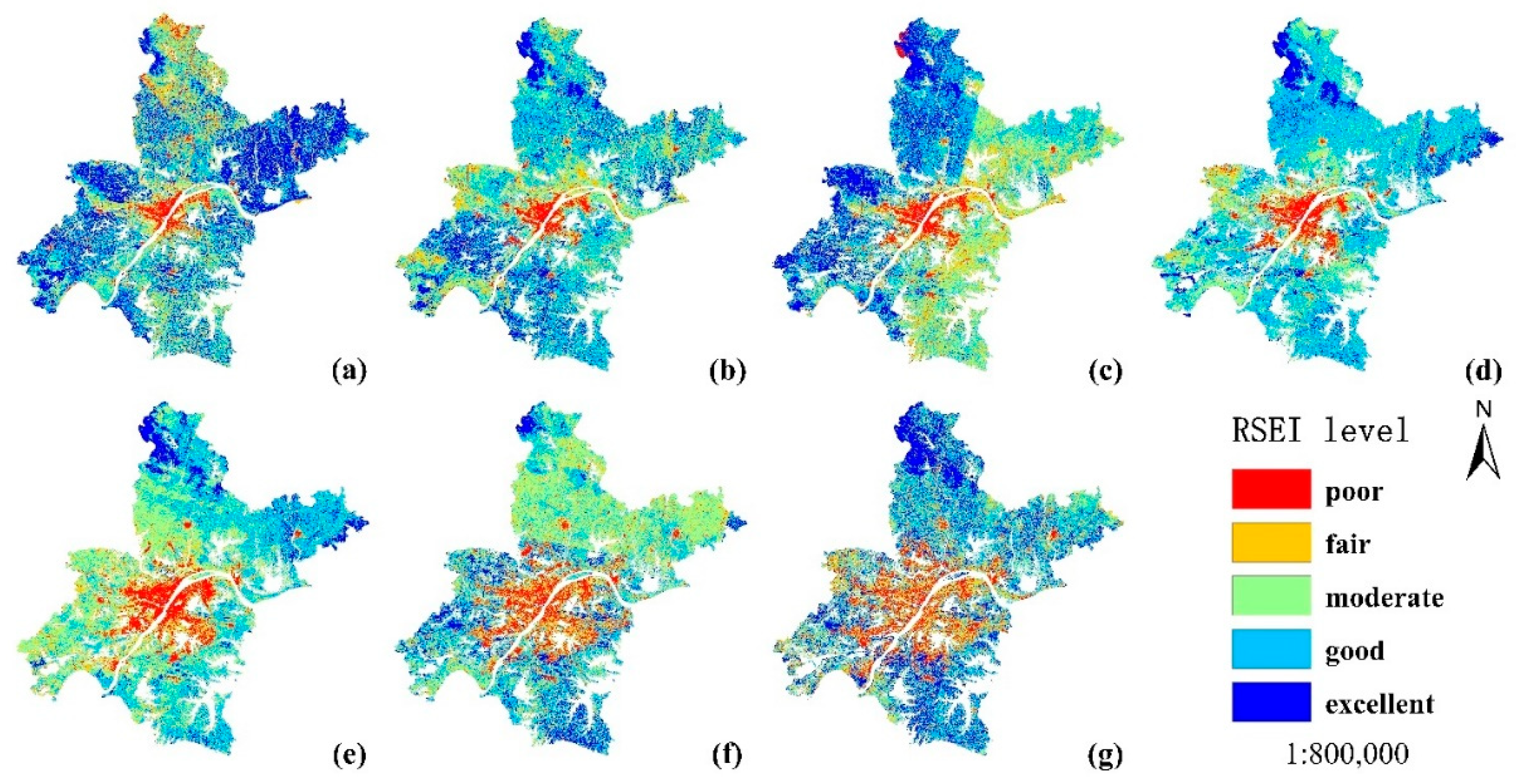
In order to provide a more visually representative depiction of the RSEI index changes in Wuhan over the past 30 years, a classification method proposed by Xu et al. was employed [11,47]. Using the method, the RSEI results in Figure 2 were divided into five levels at equal intervals; they were named, respectively, poor, fair, moderate, good, and excellent [11]. The classification outcomes are illustrated in Figure 3.
In general, from 1990 to 2020, areas with poor levels in Wuhan were mainly located in the urban region. With the expansion of central urban areas, the range of areas with poor levels has expanded. However, the clustering has decreased, especially after 2015, this trend has become more apparent. Conversely, over the last three decades, the locations in Wuhan that exhibited excellent ecological quality were mainly situated in remote urban zones. Before 2000, the main distribution area was in the West, North, and Northeast of Wuhan (Figure 3a–c). After 2000, the regions with excellent levels in Wuhan were primarily situated in the northern part of it, especially in Huangpi District in the north and Xinzhou District in the northeast. With only a few exceptions, these areas consistently maintained excellent ecological environment quality.

3.2.2. Spatial Aggregation

In this paper, five grids of different scales were created; the sizes of these grids were 1000 × 1000 m, 2000 × 2000 m, 3000 × 3000 m, 4000 × 4000 m, and 5000 × 5000 m. The RSEI values from 1990 to 2020 were extracted into the grid, and the corresponding Moran indices were calculated, respectively. The outcomes are displayed in Table 3.
Obviously, in the past three decades, the RSEI of this city has exhibited noticeable spatial aggregation characteristics at different scales. However, these characteristics have varied across different time periods and scales. Temporally, the change trends of Moran’s index for the five scales were generally consistent. From 1990 to 2010, the values kept on growing and then reached their peak in 2010. This suggested that during this period, the level of spatial clustering of poor and excellent areas in Wuhan had been increasing. In the period from 2010 to 2020, there was a declining trend, indicating a level reduction in the spatial clustering of poor and excellent areas. In terms of scale, with the increase in scale, the Moran’s index corresponding to each year had been gradually decreasing. This indicates that an increase in the time interval between samples corresponded with a higher level of information sharing between the sampled locations. Additionally, if the delay grew too substantial, spatial autocorrelation would no longer be detectable due to the loss of information.

3.2.3. Characteristics of Quantitative Changes

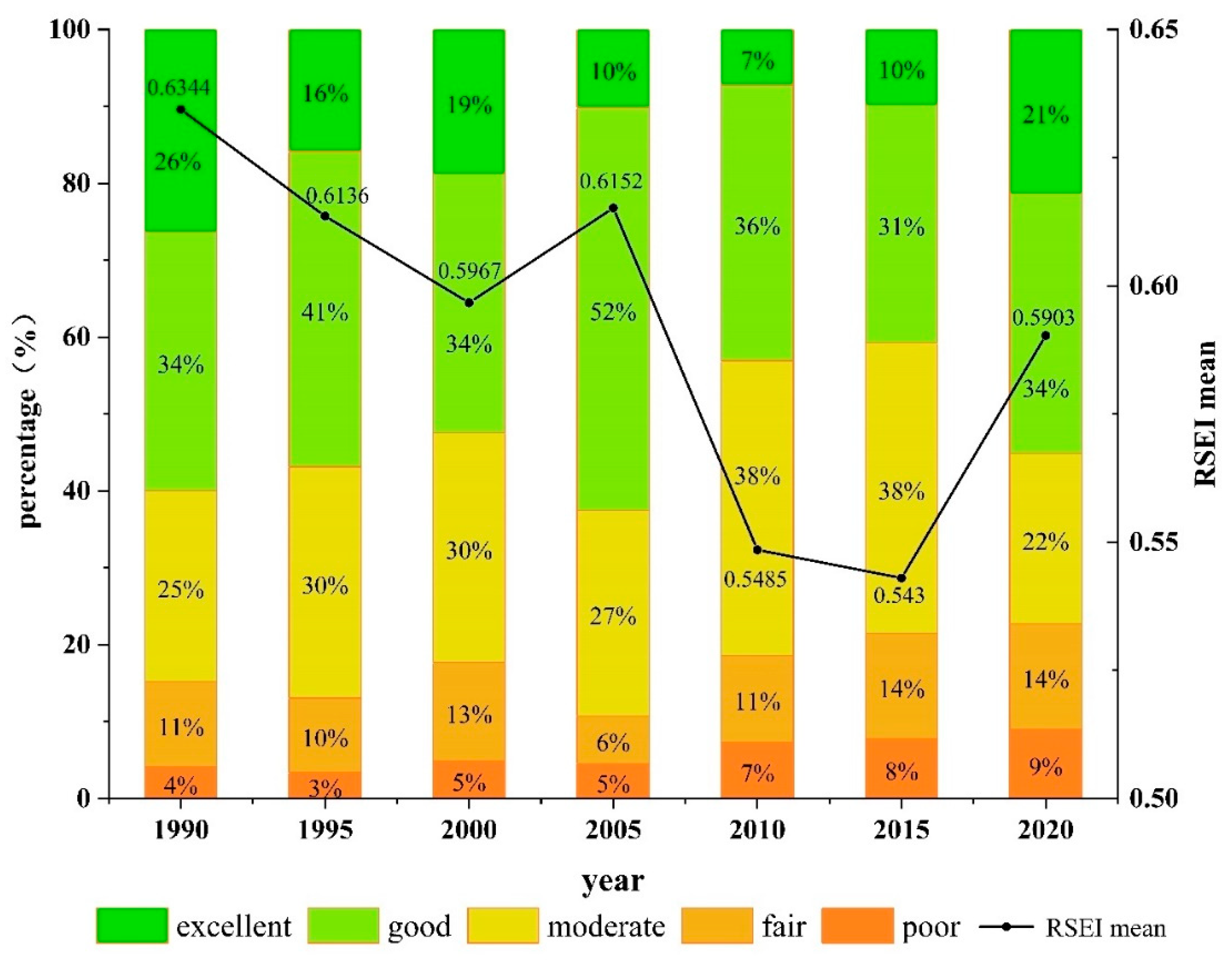
In Figure 4, the change in the average value of RSEI and the proportion of areas with different RSEI levels are illustrated. In the past three decades, the average value of RSEI in Wuhan has exhibited a fluctuating decline until 2015, having decreased from 0.6344 in 1990 to 0.5430 in 2015. Then, the average value of RSEI rebounded between 2015 and 2020, reaching 0.5903 in 2020. Examining the area proportion of different ecological quality levels, the area proportion of regions with poor levels in Wuhan has shown a steady upward trend, having increased from 4% in 1990 to 9% in 2020. The area proportion of regions with a fair level also displayed slow but consistent growth, having risen from 11% to 14% over the last 30 years. The area proportion of regions with medium ecological quality demonstrated a general trend of initial growth, having improved from 25% in 1990 to 38% in 2010, followed by a gradual decrease to 22% in 2020. The area proportion of regions with a good level had fluctuated over the period, having maintained a level of 34% both in 1990 and 2020. Notably, the area proportion of regions with excellent ecological environment quality accounted for 26% in 1990. Over the following two decades, this percentage experienced a fluctuating downward trend, reaching its lowest value of 7% in 2010. Subsequently, in 2015 and 2020, it rose to 10% and 21%, respectively, indicating a steady upward trend. This suggested that the emphasis on ecological environment protection had yielded positive results in the subsequent phases of urbanization development.

3.2.4. Characteristics of RSEI Area Transfer by Class

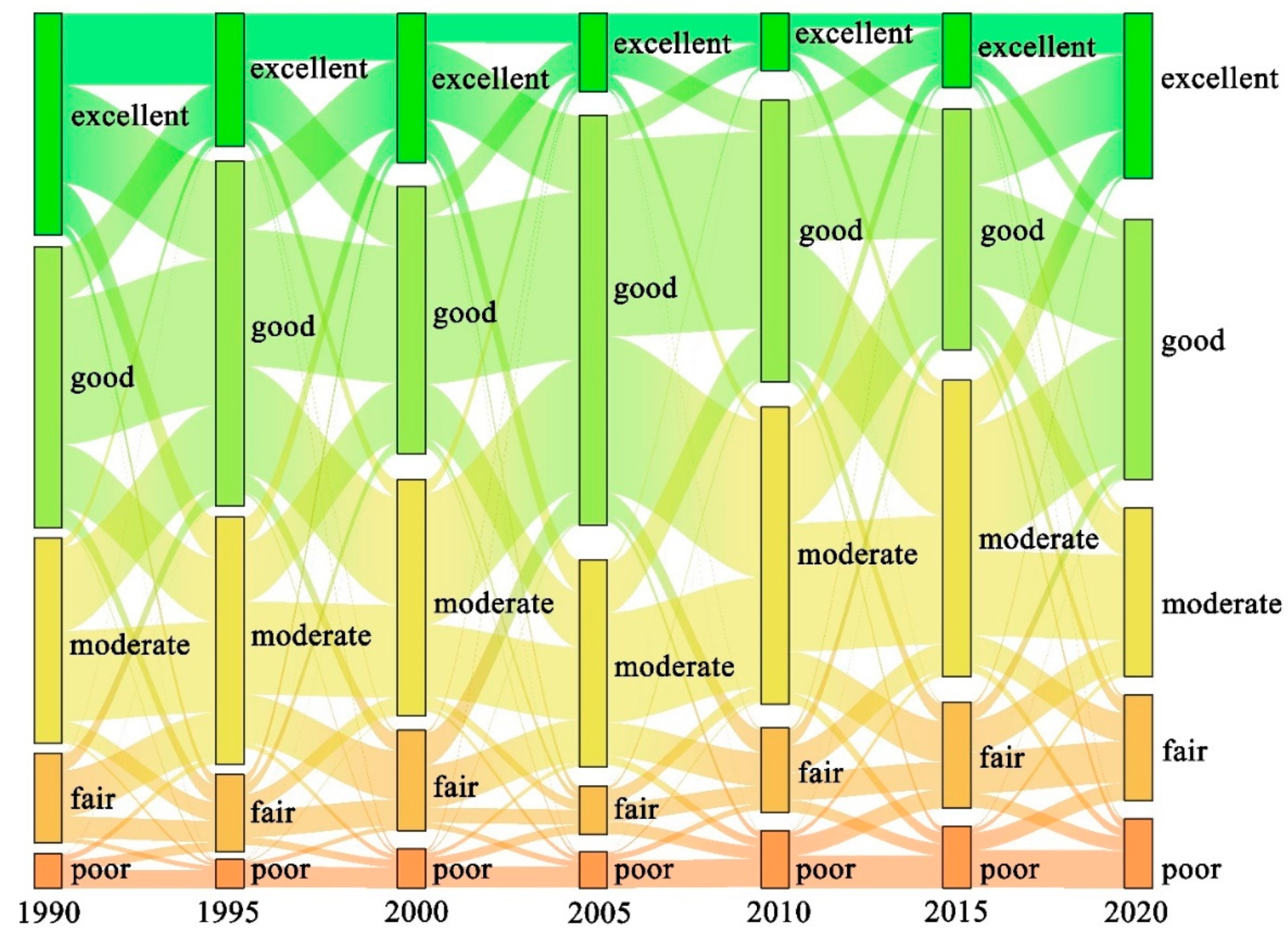
Figure 5 illustrates the mutual transfer between RSEI levels in different years. During the period from 1990 to 2000, the types of transfer between RSEI levels were primarily characterized by shifting from excellent to good, good to medium, and medium to fair. These transfers resulted in an overall decrease in RSEI during this period. From 2000 to 2005, although a large portion of the area had shifted from excellent to good, there was still more area that had shifted from moderate to good, resulting in an overall increase in RSEI during this period.
During the period from 2005 to 2015, the shift from good to moderate was the main direction of transfer, leading to a downward trend in overall RSEI during this period. In the period from 2015 to 2020, there had been a significant increase in the proportion of areas transferred from good to excellent and from medium to good, which resulted in a notable and rapid increase in Wuhan’s overall RSEI during this period.

3.3. Influencing Factor Analysis by Geodetectors

Here, we applied Geodetector to investigate which factors would affect RSEI and how significant the impact would be. These factors involved physical geography factors such as annual average precipitation, annual average temperature, elevation, and slope, as well as factors reflecting socio-economic development and human activities, including land use, GDP, population density, and location. Their sources and the relevant data are detailed in Table 1. After calculation, the explanatory power of factors for each year was shown in Table 4.
For the period 1990–2020, the p-values for all eight influencing factors on RSEI in Wuhan were 0, indicating that these factors significantly affected RSEI. From the table, the average q value of land use was 0.3136, which was the maximum mean. Followed by population density, GDP, and location, the average q-values were 0.1439, 0.1336, and 0.1092, respectively. The q-values for annual average temperature, annual average precipitation, elevation, and slope were even smaller. Land use, population density, GDP, location, annual average temperature, annual average precipitation, elevation, and slope ranked highest in terms of explanatory power according to the q values. This indicated that the primary factors influencing the ecological quality in Wuhan were related to human activities and socio-economic factors, including land use, population density, location, and GDP; climatic factors had the second-largest impact, while topographic factors had the smallest influence.
From a temporal perspective, the explanatory power (q-values) of these eight influencing factors had undergone fluctuations, initially increasing and then decreasing over the past 30 years, with all reaching their peak values in 2010. This trend was attributed to the most pronounced spatial clustering characteristics of RSEI in Wuhan in 2010, which resulted in smaller variance within each spatially heterogeneous region, thereby causing the q-values to reach their maximum.
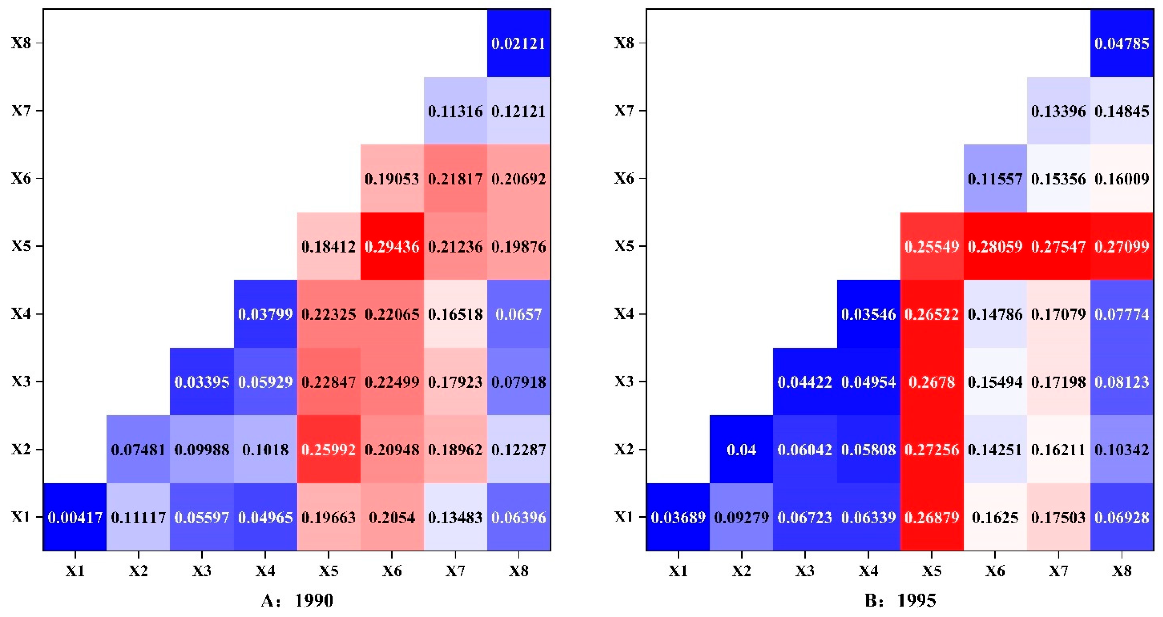
Figure 6 presents the interaction outcomes between two different factors being computed by the interaction detector. In this context, X1–X8 represented annual average precipitation, annual average temperature, elevation, slope, land use, GDP, population density, and location, respectively.
As depicted in Figure 6, the impacts of all interactions between two factors on RSEI exhibited dual-factor enhancement or non-linear amplification, with the quantity of non-linearly enhanced combinations varying across different years. Additionally, the interactions between natural and human factors surpassed the interactions between two single type factors, aligning with previous research findings [48]. For instance, there were 17 instances of non-linearly enhanced combinations in 1990. Among these, the impacts of interactions between annual average precipitation and the remaining seven factors were non-linear enhancement, and the impacts of some other interactions, for example, between annual average temperature and land use, population density, and location, between elevation and land use, GDP, population density, and location, between slope and land use, population density, and location, were non-linear enhancement too. Notably, 14 of these combinations involved the non-linear enhancement resulting from the interaction between natural and human factors. In 2015, a total of 14 non-linearly enhanced combinations were identified. For example, the impacts of interactions between annual average precipitation and annual average temperature, elevation, and slope, between annual average temperature and elevation, land use, GDP, population density, and location, between elevation and GDP, population density, and location, between slope and GDP, population density, and location, were all non-linear enhancements. In this case, 10 groups of non-linearly enhanced combinations were attributed to the interaction of natural and human factors.
In terms of the explanatory power of interactions, the most pronounced interactions at each time period over the past 30 years were observed between land use and GDP (1990, 1995), land use and annual average temperature (2000), land use and location (2005, 2010), land use and GDP (2015), and land use and slope (2020), with corresponding q-values of 0.2943, 0.2806, 0.3168, 0.4593, 0.5412, 0.3853, and 0.3568. Notably, the interaction between land use and location exhibited the highest strength, and the interactions between land use and GDP occurred most frequently. Additionally, the interactions between land use, topography, and climate were also prominently evident. Therefore, from an interaction perspective, the combined impacts between land use and other factors were poised to further magnify their influences on RSEI.

3.4. Influencing Factor Analysis by PLS-SEM

Using Geodetector, the preceding section delved into the impacts of single-factor and two-factor interactions on the spatial differentiation of RSEI in Wuhan. To further dissect the influence of different types of factors on RSEI, the SEM method was used in this section. The eight aforementioned factors were categorized into four latent variables, namely climate, terrain, humanity, and urbanization.
In PLS-SEM, using a collinearity test for factors was necessary, and the variance inflation factor (VIF) was employed to assess the collinearity; its value should ideally be close to three or lower [49]. The VIF test results are presented in Table 5.
From the table, all the VIF values were close to or less than three, suggesting that the collinearity issue was in an ideal state. The null value pertained to the path validity test failure or excessively low path coefficients. The path validity test results were presented in Table 6. Obviously, all results were statistically significant.
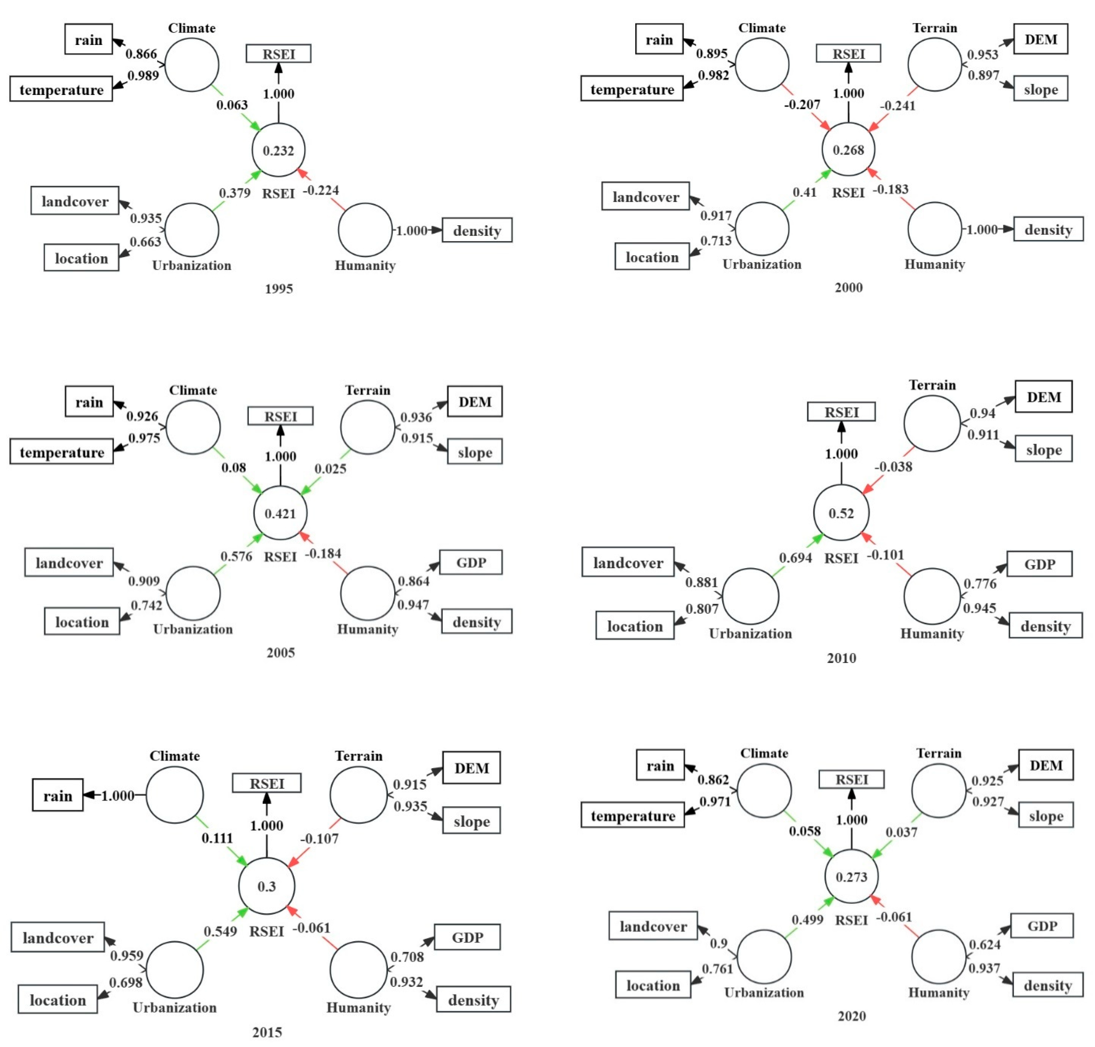
In addition, a validity and reliability examination was necessary for PLS-SEM [50]. Here, Composite Reliability (CR) was utilized to assess the internal consistency reliability, with a general expectation of no less than 0.6 [51]. The discriminant validity was decided by the Average Variance Extracted (AVE), and an AVE value that exceeded 0.5 was considered acceptable [52]. From Table 7, all the indicator values surpassed the recommended values, so the model was reliable. The SEM model established for different years is illustrated in Figure 7.
Based on the established model, it was evident that climate, topography, urbanization, and human variables exerted different influences on RSEI in various ways. Considering the explanatory power of these models, the values for 1995, 2000, 2005, 2010, 2015, and 2020 were 0.232, 0.268, 0.421, 0.520, 0.3, and 0.273, respectively. Notably, the highest explanatory power was 0.520, indicating that the four latent variables could effectively elucidate the formation mechanism of RSEI in Wuhan.
Throughout all time periods, the path coefficients of the urbanization variable consistently remained positive, indicating a positive impact of urbanization on the distribution of RSEI. The magnitude of the path coefficient fluctuated over time, reaching its peak at 0.694 in 2010, signifying that the influence of the urbanization variable on RSEI attained its maximum in that year. Conversely, the path coefficients of the human variable consistently maintained a negative value, indicating a reverse impact on the distribution of RSEI. The absolute values of these coefficients were relatively small, peaking at 0.244 in 1995 and exhibiting a decreasing trend in subsequent years. The path coefficients of the climate and terrain variables exhibited both positive and negative values at different time periods. Specifically, the coefficients of the climate variable were negative in 2000 and positive in the remaining years, suggesting a positive impact on RSEI in 2000 and a negative impact in subsequent years. The coefficients of the terrain variable displayed negative values in 2000, 2010, and 2015, indicating a negative influence on RSEI during these years, while the remaining years exhibited positive values, implying a positive impact on RSEI. The absolute values of the path coefficients for these two variables were generally small, consistently falling below 0.1 in most years.
Table 7 revealed that all the observed models for different years met the requirements for validity and reliability, which indicated that the loadings of each observed variable on the latent variables were significant. Considering the loadings of individual observational variables on the latent variables, both annual average precipitation and annual average temperature exhibited large loadings on the climate variables. Similarly, DEM and slope showed significant loadings on the terrain variables, suggesting that these observational variables possessed strong explanatory power for the latent variables. Within the remaining two latent variables, the loadings of land use on the urbanization variable mostly exceeded 0.9, while the loadings of location were slightly lower, with a minimum value of 0.663. Furthermore, the loadings of population density on the human variable consistently surpassed 0.9, and the loadings of GDP were slightly lower, with a minimum value of 0.624. Consequently, the observed variables demonstrated a commendable ability to elucidate the latent variables.

4. Discussion

4.1. Spatio-Temporal Distribution of Ecological Environment Quality

From the overall trend of change, the ecological environment quality in Wuhan exhibited a downward trajectory from 1990 to 2020. Among them, the 2000–2020 period shows a decreasing and then improving trend, which is in line with previous studies’ findings [53]. The RSEI index had declined from 0.6334 in 1990 to 0.5903 in 2020, aligning with the current scenario of escalating urban construction land and rapid urbanization. However, there were also fluctuations within this process. In the period from 2000 to 2005, the RSEI had grown from 0.5967 to 0.6152, which indicated that ecological environment quality in Wuhan had a notable improvement. During this timeframe, Wuhan accelerated its efforts in the construction of a landscape garden city, emphasizing ecological restoration through projects such as mountain greening, road landscape enhancements, and the transformation of waterfront parks.
Notable projects, such as the completion of Jiangtan Park and the Serpentine Hill re-greening in 2002, introduced significant green spaces. From 2015 to 2020, Wuhan witnessed an increase in RSEI from 0.543 to 0.5903. During this period, the city intensified its endeavors in ecological garden city construction, promoting land greening on a large scale, reinforcing landscape greening initiatives, and advancing social greening measures. These efforts collectively contributed to the enhancement of overall ecological environment quality.
From spatial distribution, the center urban areas exhibited a high concentration of regions with poor levels, gradually expanding towards the periphery over time. Similarly, in the suburban areas, where the county towns served as central points, the areas exhibiting poor levels were gradually on the rise. Conversely, regions showcasing excellent or good levels in most years were predominantly distributed in northern Huangpi District, northeastern Xinzhou District, and southern Jiangxia District. These districts, situated on the outskirts of Wuhan, were originally characterized as traditional agricultural production areas. In recent years, they have undergone substantial development in the tourism industry, leveraging their natural resource endowments. Consequently, they had maintained excellent ecological quality for the majority of the time, with only a few exceptions. Furthermore, as ecological protection and restoration efforts intensified in the central urban areas in recent years, there were also small, well-maintained pockets of ecological excellence.
In terms of spatial clustering characteristics, the RSEI in Wuhan showed significant spatial clustering in all examined years. From 1990 to 2010, the global Moran index exhibited a consistent increase, signifying a gradual enhancement in RSEI clustering. This trend could be attributed, on the one hand, to the incremental expansion of urbanized areas, resulting in an increased concentration of regions with poor levels and, on the other hand, to the concentrated distribution of regions with both excellent and good levels. However, from 2010 to 2020, the global Moran index gradually decreased, indicating a diminishing trend in RSEI clustering. This reduction was primarily attributed to the escalating fragmentation of land types resulting from urbanization and the deepening efforts in ecological management.

4.2. Single-Factor Impact and the Interactive Effects of Dual Factors

Geodetectors have been widely used in research because they can detect associations between dependent variables and other influences. In our work, a Geodetector was used to examine the influence of individual factors on the quality of the ecological environment in Wuhan. Furthermore, it could detect the interaction effects between two factors. Our results revealed that all eight factors significantly impacted the quality of the ecological environment in Wuhan. Among these factors, land use exerted the greatest influence, followed by population density, GDP, and location, indicating that anthropogenic disturbances play a primary role in influencing the ecological environment. While natural geographical factors such as annual average precipitation, annual average temperature, DEM, and slope also exhibited significant influences on ecological environment quality in Wuhan, their influence was relatively minor. From a theoretical perspective, climate and topography were expected to be crucial factors influencing ecological quality, but the impact of these natural conditions on the environment should be generally more pronounced at larger spatial and temporal scales and weaker than anthropogenic disturbances at smaller spatial and temporal scales. This observation could account for the limited explanatory power of climate and topography factors in this study.
Analyzing the outcomes of two-factor interactions, it was evident that all factors exhibited a two-factor enhancement or non-linear enhancement in their impact on ecological environment quality in Wuhan, and the interactions between natural and human factors were more pronounced than the interactions between two factors of the same type. This conclusion is in accordance with the previous findings [48]. However, because the influence of human factors was relatively greater, the interaction effect between them was more obvious. To enhance ecological environment quality, the effects of two-factor interactions should be taken into consideration, and adopting suitable combinations of these factors could lead to more favorable outcomes.

4.3. Latent Variables Influence

Geodetector can only explain whether the factors are significant to RSEI’s spatial distribution in Wuhan and cannot measure each factor’s contribution to the value of RSEI, which is usually explored in studies frequently using MGWR [54] or GWR [12], and less for SEM modeling. To examine the influence of various variables on RSEI, SEM was employed in this study. Although the SEM models established here were complete only for the years 2005 and 2020, and models for other years lacked some influencing factors due to validity concerns, it maintained data continuity with minimal impact on the results. The findings revealed that the structural models established for each year met reliability and significance requirements, and all four latent variables exhibited a significant influence on the RSEI index of Wuhan.
In this paper, when reclassifying land use data, some types of land, such as impervious surfaces and unused land, that had a negative impact on RSEI were assigned lower values, while forests, grasslands, and other categories with a positive influence on RSEI were assigned higher values. Additionally, closer areas to the urban built-up zone were assigned lower values, whereas more distant areas received higher values. Consequently, the urbanization variable exhibited a consistently positive influence on RSEI across various time periods, displaying the highest path coefficient. Hence, this variable had the greatest impact on RSEI. The path coefficients for the human variable were all negative, which indicated that the rise in population density and regional GDP development would exert pressure on the ecological environment. According to the changing trend of these path coefficients, the influence of human variables was diminishing year by year, which signified that people tried to avoid ecological damage in the process of population and economic development.
Here, climate and terrain variables exhibited varying directions of influence on RSEI across different time periods. Two potential reasons might account for this phenomenon. Firstly, from a terrain perspective, the average elevation in Wuhan was a mere 23.3 m. Low-elevation and gently sloping terrain were predominant, which was conducive to human activities. Combined with different climate factors in various years, this kind of terrain could yield diverse impacts on vegetation growth, thereby affecting the quality of the ecological environment. Secondly, the majority of absolute values of path coefficients for climate and terrain variables were relatively small, so small measurement errors and disturbances could affect their value direction.
In this paper, the impact of some factors on RSEI in Wuhan has been explored, and the results prove to be effective. In fact, there are additional natural and human geographic factors, such as sunshine and distance from roads, that could potentially influence RSEI. In future research, these factors will be used, which should enhance the accuracy of the results. Moreover, alternative models and algorithms will be employed for comprehensive evaluation, aiming to achieve a more comprehensive assessment of regional ecological environment quality.

5. Conclusions

The ecological environment quality of Wuhan was assessed by calculating the RSEI index, and the spatiotemporal distribution characteristics of it were analyzed. Using Geodetectors and SEM models, the influences of climate, terrain, urbanization, and human factors on Wuhan’s ecological environment quality were explored from various perspectives. Some conclusions were drawn, as described below.
In the past 30 years, the overall ecological environment quality in Wuhan has shown a fluctuating downward trend, experiencing a noticeable decline from 1990 to 2015, followed by a gradual upward trend after 2015. A fluctuating developmental pattern has also been followed by the percentage of areas with a good or excellent level, while the area of regions with a poor level has consistently risen. Analyzing the spatial distribution, regions with poor levels were predominantly situated in county towns and central urban areas, whereas areas with good and excellent ecological conditions were primarily located in distant urban sectors, such as the north, northeast, and south, displaying significant clustering characteristics.
Wuhan’s ecological environment quality is impacted by several variables the most important impact was exerted by land use, followed by population density, GDP, and location. This suggested that ecological quality’s primary influencers were human geographic factors. Significant impact, including annual average temperature, annual average precipitation, elevation, and slope, was also exhibited by natural geographic factors on ecological environment quality, albeit with relatively less influence. In interaction detection’s results, the interaction degree was surpassed by the interaction degree between natural factors and human factors between factors in the same category individually. The four integrated factors, namely urbanization, humans, climate, and terrain, also wield substantial influence on the ecological environment quality in Wuhan.
Therefore, to improve the quality of the ecological environment, we must make more reasonable use of land resources in urban planning and construction, accelerate the construction of urban parks and other facilities, expand the urban green area, and reduce human activities that disrupt the ecological environment. Reversing the trend of increasing areas with poor ecological quality, improving the urban ecological quality in central districts, and maintaining well-preserved regions will contribute to the positive development of ecological quality in Wuhan.

Author Contributions

Conceptualization, X.G. and X.D.; methodology, X.G. and X.D.; validation, X.G.; formal analysis, X.G.; investigation, X.G.; writing—original draft preparation, X.G. writing—review and editing, X.D.; visualization, X.G.; supervision, X.D.; project administration, X.D., C.D. and L.P. All authors have read and agreed to the published version of the manuscript.

Funding

This study was supported by the National Natural Science Foundation of China under Grant No. 41971402.

Institutional Review Board Statement

Not applicable.

Informed Consent Statement

Not applicable.

Data Availability Statement

The data used in this study can be obtained from the first author at [email protected] with a reasonable request.

Acknowledgments

The Landsat TM and Landsat OLI images were from USGS, which provides an open database. The authors would like to thank the above institutions for their help and support.

Conflicts of Interest

The authors declare no conflicts of interest.

References

  1. Chen, Y.P.; Ren, J.; Wang, L. Review on monitoring method of ecological conservation and restoration project area based on multi-source remote sensing data. Acta Ecol. Sin. 2019, 39, 8789–8797. [Google Scholar]
  2. Avdan, Z.Y.; Kaplan, G.; Goncu, S.; Avdan, U. Monitoring the Water Quality of Small Water Bodies Using High- Resolution Remote Sensing Data. ISPRS Int. J. Geo-Inf. 2019, 8, 553. [Google Scholar] [CrossRef]
  3. Gleason, C.J.; Durand, M.T. Remote Sensing of River Discharge: A Review and a Framing for the Discipline. Remote Sens. 2020, 12, 1107. [Google Scholar] [CrossRef]
  4. Gupta, K.; Kumar, P.; Pathan, S.K.; Sharma, K.P. Urban Neighborhood Green Index-A measure of green spaces in urban areas. Landsc. Urban Plan. 2012, 105, 325–335. [Google Scholar] [CrossRef]
  5. Vits, E.; Cherlet, M.; Mehl, W.; Sommer, S. Estimating the ecological status and change of riparian zones in Andalusia assessed by multi-temporal AVHHR datasets. Ecol. Indic. 2009, 9, 422–431. [Google Scholar] [CrossRef]
  6. Moran, M.S.; Peters-Lidard, C.D.; Watts, J.M.; McElroy, S. Estimating soil moisture at the watershed scale with satellite-based radar and land surface models. Can. J. Remote Sens. 2004, 30, 805–826. [Google Scholar] [CrossRef]
  7. Wang, M.Y.; Xu, H.Q. Temporal and spatial changes of urban impervious surface and its influence on urban ecological quality: A comparison between Shanghai and New York. Chin. J. Appl. Ecol. 2018, 29, 3735–3746. [Google Scholar]
  8. Han, D.; Zhang, W.J.; Li, Q.; Liu, X.; Deng, Y.; Zhou, W. Study on the Relationship between the Impervious Surface Expansion and the Change of Ecological Environment Quality in Chengdu. J. Southwest Univ. Sci. Technol. 2019, 34, 34–40. [Google Scholar]
  9. Li, Y.L.; Wang, X.Q.; Chen, Y.Z.; Wang, M.M. The correlation analysis of land surface temperature and fractional vegetation coverage in Fujian Province. J. Geo-Inf. Sci. 2019, 21, 445–454. [Google Scholar]
  10. Imhoff, M.L.; Zhang, P.; Wolfe, R.E.; Bounoua, L. Remote sensing of the urban heat island effect across biomes in the continental, U.S.A. Remote Sens. Environ. 2010, 114, 504–513. [Google Scholar] [CrossRef]
  11. Xu, H.Q. A remote sensing urban ecological index and its application. Acta Ecol. Sin. 2013, 33, 7853–7862. [Google Scholar]
  12. Geng, J.; Yu, K.; Xie, Z.; Zhao, G.; Ai, J.; Yang, L.; Yang, H.; Liu, J. Analysis of Spatiotemporal Variation and Drivers of Ecological Quality in Fuzhou Based on RSEI. Remote Sens. 2022, 14, 4900. [Google Scholar] [CrossRef]
  13. Zhang, K.; Feng, R.; Zhang, Z.; Deng, C.; Zhang, H.; Liu, K. Exploring the Driving Factors of Remote Sensing Ecological Index Changes from the Perspective of Geospatial Differentiation: A Case Study of the Weihe River Basin, China. Int. J. Environ. Res. Public Health 2022, 19, 10930. [Google Scholar] [CrossRef]
  14. Yao, K.; Halike, A.; Chen, L.; Wei, Q. Spatiotemporal changes of eco-environmental quality based on remote sensing-based ecological index in the Hotan Oasis, Xinjiang. J. Arid Land 2022, 14, 262–283. [Google Scholar] [CrossRef]
  15. Duan, Q.; Tan, M. Using a geographical detector to identify the key factors that influence urban forest spatial differences within China. Urban For. Urban Green. 2020, 49, 126623. [Google Scholar] [CrossRef]
  16. Ren, Y.W.; Cao, W.D.; Zhang, Y.; Su, H.F.; Wang, X.W. Temporal and Spatial Coupling Characteristics of Urbanization and Ecological Environment of Three Major Urban Agglomerations in the Yangtze River Economic Belt. Resour. Environ. Yangtze Basin 2019, 28, 2586–2600. [Google Scholar]
  17. Zhou, Z.L.; Sha, J.M.; Fan, Y.X.; Shuai, C.; Gao, S. Temporal and Spatial variations of impervious surface landscape pattern and the driving factors in Xiamen City, China. Chin. J. Appl. Ecol. 2020, 31, 230–238. [Google Scholar]
  18. Zhu, Q.; Guo, J.X.; Guo, X.; Xu, Z.; Ding, H.; Han, Y. Spatial variations of ecological environment quality and its influencing factors in Poyang Lake area, Jiangxi, China. Chin. J. Appl. Ecol. 2019, 30, 4108–4116. [Google Scholar]
  19. Fotheringham, A.S.; Charlton, M.; Brunsdon, C. The geography of parameter space: An investigation into spatial non-stationarity. Int. J. Geogr. Inf. Syst. 1996, 10, 605–627. [Google Scholar] [CrossRef]
  20. Brunsdon, C.; Fotheringham, A.S.; Charlton, M. Geographically weighted Regression: A method for Exploring Spatial Non-stationarity. Geogr. Anal. 1996, 28, 281–298. [Google Scholar] [CrossRef]
  21. Wang, J.F.; Li, X.H.; Christakos, G.; Liao, Y.-L.; Zhang, T.; Gu, X.; Zheng, X.-Y. Geographical detectors-based health risk assessment and its application in the neural tube defects study of the Heshun region, China. Int. J. Geogr. Inf. Sci. 2010, 24, 107–127. [Google Scholar] [CrossRef]
  22. Bai, L.M.; Feng, X.H.; Sun, R.F.; Gao, H. Spatial and temporal responses of habitat quality to urbanization: A case study of Chang-chun City, Jilin Province, China. Chin. J. Appl. Ecol. 2020, 31, 1267–1277. [Google Scholar]
  23. Liu, Y.W.; Liu, C.W.; He, Z.Y.; Zhou, X.; Han, B.H.; Hao, H.Z. Spatial-temporal evolution of ecological land and influence factors in Wuhan urban agglomeration based on geographically weighted regression model. Chin. J. Appl. Ecol. 2020, 31, 987–998. [Google Scholar]
  24. Han, Y.; Guo, X.; Jiang, Y.F.; Rao, L.; Sun, K.; Li, J.; Wang, L. Cultivated land landscape ecological security: Influencing factors and spatial differences in the hilly region of South China. Acta Ecol. Sin. 2019, 39, 6522–6533. [Google Scholar]
  25. Zhao, W.; Hu, Z.M.; Guo, Q.; Wu, G.; Chen, R.; Li, S. Contributions of Climatic Factors to Interannual Variability of the Vegetation Index in Northern China Grasslands. J. Clim. 2020, 33, 175–183. [Google Scholar] [CrossRef]
  26. Ju, H.R.; Zhang, Z.X.; Zuo, L.J.; Wang, J.; Zhang, S.; Wang, X.; Zhao, X. Driving forces and their interactions of built-up land expansion based on the geographical detector—A case study of Beijing, China. Int. J. Geogr. Inf. Sci. 2016, 30, 2188–2207. [Google Scholar] [CrossRef]
  27. A, Y.; Wang, G.; Liu, T.; Shrestha, S.; Xue, B.; Tan, Z. Vertical variations of soil water and its controlling factors based on the structural equation model in a semi-arid grassland. Sci. Total Environ. 2019, 691, 1016–1026. [Google Scholar] [CrossRef]
  28. Cortizas, A.M.; Horák-Terra, I.; Pérez-Rodríguez, M.; Bindler, R.; Cooke, C.A.; Kylander, M. Structural equation modeling of long-term controls on mercury and bromine accumulation in Pinheiro mire (Minas Gerais, Brazil). Sci. Total Environ. 2021, 757, 143940. [Google Scholar] [CrossRef]
  29. Ganesh, D.; Justin, P. CB-SEM vs PLS-SEM methods for research in social sciences and technology forecasting. Technol. Forecast. Soc. Change 2021, 173, 121092. [Google Scholar]
  30. Xie, M.; Chen, J.; Zhang, Q.; Li, H.; Fu, M.; Breuste, J. Dominant landscape indicators and their dominant areas influencing urban thermal environment based on structural equation model. Ecol. Indic. 2020, 111, 105992. [Google Scholar] [CrossRef]
  31. Simandan, D. The wise stance in human geography. Trans. Inst. Br. Geogr. 2011, 36, 188–192. [Google Scholar] [CrossRef]
  32. NASA JPL. NASADEM Merged DEM Global 1 arc second V001 [Data set]. NASA EOSDIS Land Processes DAAC. 2020. Available online: https://lpdaac.usgs.gov/products/nasadem_hgtv001/ (accessed on 28 February 2023).
  33. Yang, J.; Huang, X. 30 m annual land cover and its dynamics in China from 1990 to 2019. Earth Syst. Sci. Data Discuss. 2021, 233, 1–29. [Google Scholar]
  34. Peng, S.Z.; Gang, C.; Cao, Y.; Chen, Y. Assessment of climate change trends over the loess plateau in china from 1901 to 2100. Int. J. Climatol. 2017, 38, 2250–2264. [Google Scholar] [CrossRef]
  35. Peng, S.Z.; Ding, Y.X.; Wen, Z.M.; Chen, Y.M.; Cao, Y.; Ren, J.Y. Spatiotemporal change and trend analysis of potential evapotranspiration over the Loess Plateau of China during 2011–2100. Agric. For. Meteorol. 2017, 233, 183–194. [Google Scholar] [CrossRef]
  36. Ding, Y.X.; Peng, S.Z. Spatiotemporal trends and attribution of drought across China from 1901–2100. Sustainability 2020, 12, 477. [Google Scholar] [CrossRef]
  37. Peng, S.Z.; Ding, Y.X.; Liu, W.Z.; Li, Z. 1 km monthly temperature and precipitation dataset for China from 1901 to 2017. Earth Syst. Sci. Data 2019, 11, 1931–1946. [Google Scholar] [CrossRef]
  38. Peng, S. 1-km Monthly Mean Temperature Dataset for China (1901–2022); National Tibetan Plateau/Third Pole Environment Data Center: Beijing, China, 2019. [Google Scholar]
  39. Peng, S. 1-km Monthly Precipitation Dataset for China (1901–2022); National Tibetan Plateau/Third Pole Environment Data Center: Beijing, China, 2020. [Google Scholar]
  40. Pekel, J.F.; Cottam, A.; Gorelick, N.; Belward, A.S. High-resolution mapping of global surface water and its long-term changes. Climate 2016, 540, 418–422. [Google Scholar] [CrossRef] [PubMed]
  41. Sun, J.; Sun, Z.; Guo, H.; Xing, Q.; Du, W.; Cai, G. A dataset of built-up area of Chinese cities in 2020. China Sci. Data 2022, 7, 190–201. [Google Scholar]
  42. Nichol, J. Remote sensing of urban heat islands by day and night. Photogramm. Eng. Remote Sens. 2005, 71, 613–622. [Google Scholar] [CrossRef]
  43. Jiménez-Muñoz, J.C.; Sobrino, J.A.; Skoković, D.; Mattar, C.; Cristóbal, J. Land Surface Temperature Retrieval Methods From Landsat-8 Thermal Infrared Sensor Data. Geosci. Remote Sens. Lett. IEEE 2014, 11, 1840–1843. [Google Scholar] [CrossRef]
  44. Rikimaru, A.; Roy, P.S.; Miyatake, S. Tropical forest cover density mapping. Trop. Ecol. 2002, 43, 39–47. [Google Scholar]
  45. Wang, J.F.; Xu, C.D. Geodetector: Principle and prospective. Acta Geogr. Sin. 2017, 72, 116–134. [Google Scholar]
  46. Hair, J.F.; Howard, M.C.; Nitzl, C. Assessing measurement model quality in PLS-SEM using confirmatory composite analysis. J. Bus. Res. 2020, 109, 101–110. [Google Scholar] [CrossRef]
  47. Hu, X.; Xu, H. A new remote sensing index for assessing the spatial heterogeneity in urban ecological quality: A case from Fuzhou City, China. Ecol. Indic. 2018, 89, 11–21. [Google Scholar] [CrossRef]
  48. Chen, W.; Li, J.; Zeng, J.; Ran, D.; Yang, B. Spatial heterogeneity and formation mechanism of eco-environmental effect of land use change in China. Geogr. Res. 2019, 38, 2173–2187. [Google Scholar]
  49. Hair, J.F.; Risher, J.J.; Sarstedt, M.; Ringle, C.M. When to use and how to report the results of PLS-SEM. Eur. Bus. Rev. 2019, 31, 2–24. [Google Scholar] [CrossRef]
  50. Sarstedt, M.; Hair, J.F.; Cheah, J.-H.; Becker, J.-M.; Ringle, M.C. How to specify, estimate, and validate higher-order constructs in PLS-SEM. Australas. Mark. J. AMJ 2019, 27, 197–211. [Google Scholar] [CrossRef]
  51. Turner, G. Organisation in the school dental service. Br. Dent. J. 1971, 131. [Google Scholar]
  52. Fornell, C.; Larcker, D.F. Evaluating Structural Equation Models with Unobservable Variables and Measurement Error. J. Mark. Res. 1981, 18, 39–50. [Google Scholar] [CrossRef]
  53. Zhang, W.; Zhang, W.; Ji, J.; Chen, C. Urban Ecological Quality Assessment Based on Google Earth Engine and Driving Factors Analysis: A Case Study of Wuhan City, China. Sustainability 2024, 16, 3598. [Google Scholar] [CrossRef]
  54. Wen, C.; Zhan, Q.; Zhan, D.; Zhao, H.; Yang, C. Spatiotemporal Evolution of Lakes under Rapid Urbanization: A Case Study in Wuhan, China. Water 2021, 13, 1171. [Google Scholar] [CrossRef]
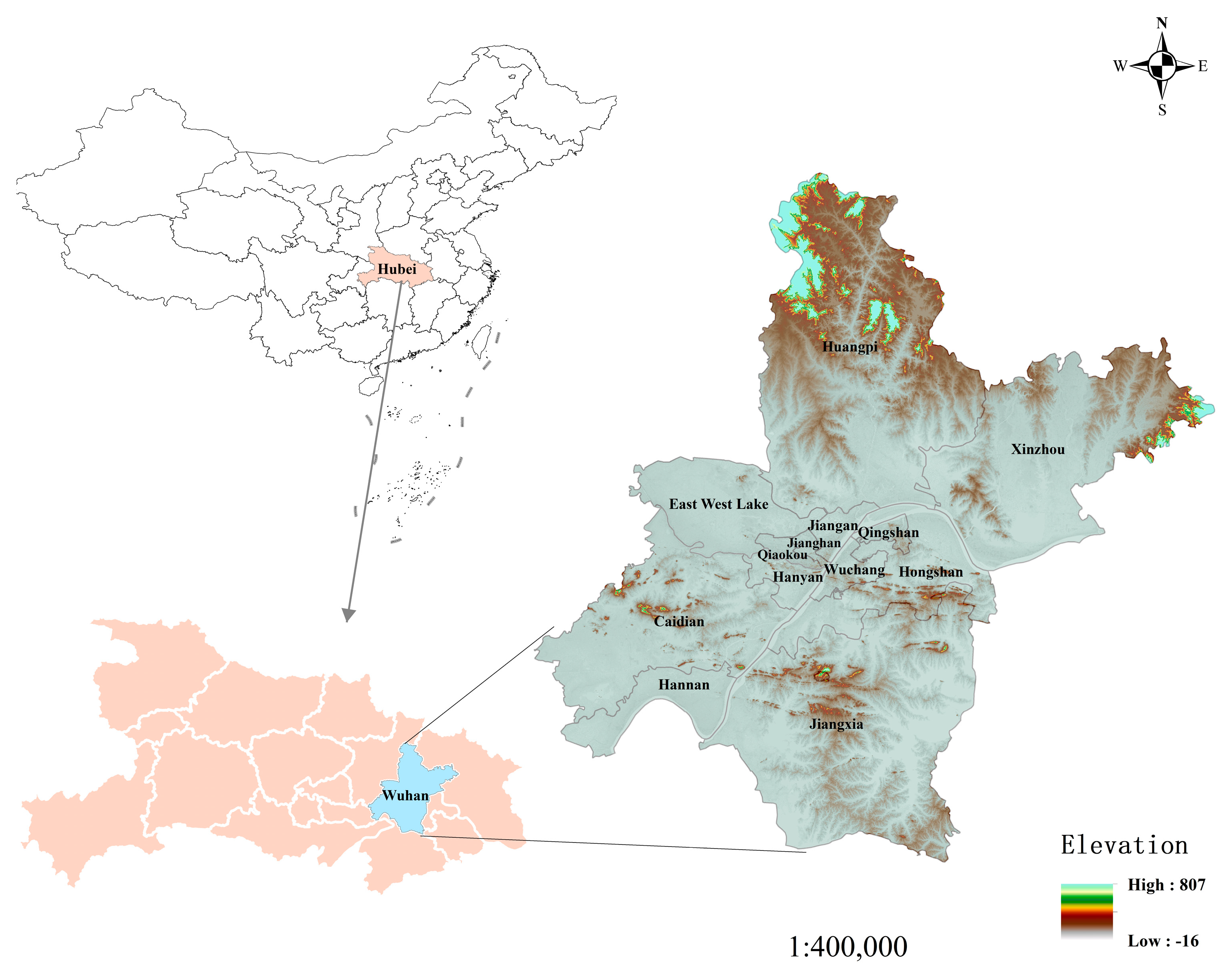
Figure 1. Location map of Wuhan City.
Sustainability 16 05809 g001
Figure 2. Map of RSEI distribution in different years (a) 1990; (b) 1995; (c) 2000; (d) 2005; (e) 2010; (f) 2015; (g) 2020.
Sustainability 16 05809 g002
Figure 3. Map of RSEI levels in different years (a) 1990; (b) 1995; (c) 2000; (d) 2005; (e) 2010; (f) 2015; (g) 2020.
Sustainability 16 05809 g003
Figure 4. Mean value of RSEI and area proportion of RSEI of each class in Wuhan, 1990–2020.
Sustainability 16 05809 g004
Figure 5. Area shift of RSEI by class in Wuhan, 1990–2020.
Sustainability 16 05809 g005
Figure 6. Detection results of the interaction of the influencing factors.
Sustainability 16 05809 g006aSustainability 16 05809 g006bSustainability 16 05809 g006c
Figure 7. Correlation between relevant influences and RSEI in the study area by year.
Sustainability 16 05809 g007
Table 1. Data source.
Data TypeData FormatResolutionSource
1990–2010 remote sensing images.tif30 mLANDSAT/LT05/C01/T1_SR
http://www.usgs.gov
(accessed on 2 March 2023)
2015–2020 remote sensing images.tif30 mLANDSAT/LC08/C01/T1_SR
http://www.usgs.gov
(accessed on 2 March 2023)
1990–2020 Wuhan water surface area.tif30 mJRC/GSW1_3/YearlyHistory [40]
(accessed on 2 March 2023)
DEM.tif30 mNASA/NASADEM_HGT/001 [32]
http://www.earthdata.nasa.gov
(accessed on 2 March 2023)
1990–2020 Wuhan landuse.tif30 mAnnual China Land Cover Dataset, CLCD [33]
1990–2020 Wuhan annual average precipitation.tif1000 mTPDC/CHINA_1KM_PRE_MONTH
http://data.tpdc.ac.cn
(accessed on 20 March 2023)
1990–2020 Wuhan annual average temperature.tif1000 mTPDC/CHINA_1KM_AVG_TEM_MONTH
http://data.tpdc.ac.cn
(accessed on 20 March 2023)
Population density.tif30 mWuhan Statistical Yearbook
https://tjj.wuhan.gov.cn/
(accessed on 20 March 2023)
GDP.tif30 mWuhan Statistical Yearbook
https://tjj.wuhan.gov.cn/
(accessed on 20 March 2023)
Location.shp-China’s 2020 built-up area dataset [41]
(accessed on 20 March 2023)
Table 2. Results of PCA.
YearIndicatorPC1PC2PC3PC4
1990NDVI0.72830.65470.01180.2015
WET0.1615−0.4213−0.38000.8074
NDBSI−0.52050.39920.51270.5538
LST−0.41520.4841−0.7697−0.0265
Eigenvalue0.02440.00990.00310.0002
Percent eigenvalue64.91%26.35%8.13%0.61%
1995NDVI0.87980.44090.09620.1491
WET0.0309−0.3311−0.19490.9227
NDBSI−0.46060.71410.39030.3542
LST−0.11300.4311−0.8946−0.0304
Eigenvalue0.02420.00970.00490.0001
Percent eigenvalue62.04%25.00%12.55%0.42%
2000NDVI0.76350.6122−0.01390.2051
WET0.1797−0.5033−0.20740.8193
NDBSI−0.56750.53580.32260.5353
LST−0.25020.2911−0.9233−0.0001
Eigenvalue0.02420.00540.00180.0001
Percent eigenvalue76.43%17.17%5.92%0.47%
2005NDVI0.8063−0.57360.1064−0.3762
WET0.05320.1662−0.3473−0.0112
NDBSI−0.3237−0.23630.8353−0.9213
LST−0.4921−0.7664−0.4126−0.0971
Eigenvalue0.01540.00320.00130.00003
Percent eigenvalue77.03%16.04%6.74%0.19%
2010NDVI0.8624−0.40770.2904−0.0748
WET0.0132−0.0092−0.2983−0.9543
NDBSI−0.21420.24170.9017−0.2871
LST−0.4593−0.88040.1162−0.0341
Eigenvalue0.01220.00460.00210.00003
Percent eigenvalue64.29%24.50%11.04%0.17%
2015NDVI0.8378−0.45040.2783−0.1331
WET0.08860.2680−0.2727−0.9197
NDBSI−0.5147−0.46720.6170−0.3687
LST−0.1588−0.7119−0.6837−0.0201
Eigenvalue0.02280.00420.00230.00009
Percent eigenvalue77.15%14.50%8.02%0.33%
2020NDVI0.8024−0.43240.3563−0.2053
WET0.15190.2916−0.4626−0.8232
NDBSI−0.5386−0.24820.6072−0.5286
LST−0.206−0.8162−0.5387−0.0246
Eigenvalue0.04210.00390.00280.0002
Percent eigenvalue85.78%8.06%5.70%0.46%
Table 3. RSEI Moran index at different scales.
Scale (m)Moran’s I
1990199520002005201020152020
10000.3410.3760.5130.540.5730.330.331
20000.2670.2760.4520.4410.4950.2810.267
30000.2530.2590.4720.3850.4760.2630.218
40000.2250.2920.3930.4440.460.1570.148
50000.1180.1770.3020.3780.3880.2080.233
Note: All indices in the table have a p-value of 0.
Table 4. Explanatory power (q-value) of each factor on RSEI.
YearAnnual Average PrecipitationAnnual Average TemperatureElevationSlopeLanduseGDPPopulation DensityLocation
19900.00420.07480.0340.0380.18410.19050.11320.0212
19950.0370.040.04420.03550.25550.11560.13390.0479
20000.03190.13820.02660.02350.23550.10780.15290.0781
20050.11660.08690.10920.08040.41310.1760.20920.16
20100.15230.19870.14450.09290.4570.19330.22410.2759
20150.05450.01260.02980.03180.33260.0890.08930.0559
20200.09730.05920.0770.06260.31740.06310.08480.1256
Mean0.07050.08720.06650.05210.31360.13360.14390.1092
Note: The p-values for the indicators in the table are 0.
Table 5. PLS-SEM model variance inflation factors for each indicator.
VIF199520002005201020152020
Annual average precipitation2.5762.7053.031-1.0002.050
Annual average temperature2.5762.7053.031--2.050
Elevation-2.0752.0482.0522.0342.049
Slope-2.0752.0482.0522.0342.049
Landuse1.1441.1631.1841.2291.2761.192
GDP1.000-1.7591.3851.1961.109
Population density1.0001.0001.7591.3851.1961.109
Location1.1441.0001.1841.2291.2761.192
Table 6. Results of the path validity test.
YearPathPath Coefficientp Value
1995Climate → RSEI0.0680.000
Humanity → RSEI−0.2270.000
Urbanization → RSEI0.370.000
2000Climate → RSEI−0.2070.000
Terrain → RSEI−0.2410.000
Humanity → RSEI−0.1830.000
Urbanization → RSEI0.410.000
2005Climate → RSEI0.080.000
Terrain → RSEI0.0250.028
Humanity → RSEI−0.1840.000
Urbanization → RSEI0.5760.000
2010Terrain → RSEI−0.0380.000
Humanity → RSEI−0.1010.000
Urbanization → RSEI0.6940.000
2015Climate → RSEI0.1110.000
Terrain → RSEI−0.1070.000
Humanity → RSEI−0.0610.000
Urbanization → RSEI0.5490.000
2020Climate → RSEI0.0580.000
Terrain → RSEI0.0370.000
Humanity → RSEI−0.0610.000
Urbanization → RSEI0.4990.000
Table 7. PLS-SEM reliability assessment.
YearVariablesCR ValueAVE Value
1995Climate0.9260.864
Urbanization0.7880.657
2000Climate0.9380.883
Terrain0.9220.856
Urbanization0.8030.675
2005Climate0.9490.904
Terrain0.9230.857
Urbanization0.8140.688
Humanity0.9020.822
2010Terrain0.9230.857
Urbanization0.8330.714
Humanity0.8540.748
2015Terrain0.9220.856
Urbanization0.8220.703
Humanity0.810.685
2020Climate0.9150.843
Terrain0.9230.858
Urbanization0.8180.694
Humanity0.7690.634
Disclaimer/Publisher’s Note: The statements, opinions and data contained in all publications are solely those of the individual author(s) and contributor(s) and not of MDPI and/or the editor(s). MDPI and/or the editor(s) disclaim responsibility for any injury to people or property resulting from any ideas, methods, instructions or products referred to in the content.