Abstract
The Pareto frontier, a concept rooted in economics and multi-objective optimization, represents the interplay between two objectives. In the context of power systems, it is often the case that different objectives have to be considered at the same time, such as the minimization of the operational cost and the minimization of greenhouse gas emissions. However, whether both objectives are achievable or not largely depends on the specific technoeconomic characteristics of the generation units involved. In this context, the current paper presents the Pareto frontier for different combinations of technoeconomic characteristics of generation units, and different types of functions for the operational cost and CO2 emissions, as well as various technologies, including Combined Heat and Power, heat-only and thermal power stations. The analysis reveals a range of shapes for the resulting Pareto frontier and underlines the critical patterns and dependencies within the energy system’s operational framework, highlighting the complex interplay between environmental impact and economic feasibility.
1. Introduction
The energy sector stands at a crucial intersection of economic viability, environmental responsibility, and technological innovation. As the global energy demand continues to rise, the need to optimize energy systems for efficiency, cost, and environmental impact becomes increasingly paramount. This paper delves into the complex subject of multi-objective optimization in energy systems, employing the Pareto frontier analysis as a pivotal tool to navigate the intricate trade-offs inherent in this field.
At the core of this study lies the Pareto frontier, a concept borrowed from economics and adapted to the multifaceted objectives of heat and power generation. This frontier represents a combination of optimal solutions where no single objective can be improved without compromising another. In the context of energy systems, these objectives typically revolve around operational costs and environmental impacts, such as CO2 emissions. The Pareto frontier thus emerges as an invaluable analytical tool, enabling the identification of the most effective combinations of generation technologies under varying conditions and constraints.
Since renewables do not cause greenhouse gas emissions, the current work focuses on the technologies that do emit, namely thermal power stations, heat-only units, and combined heat and power stations (CHPs). These technologies represent the diversity of current energy generation methods, each with unique operational characteristics, and environmental footprints. Thermal power units, largely driven by the combustion of fossil fuels, remain a cornerstone of energy supply but are increasingly scrutinized for their environmental impact. Heat-only units, on the other hand, specialize in providing heating but lack the capability of power generation. CHP units represent a more holistic approach, simultaneously generating electricity and useful heat, exhibiting enhanced overall efficiency. The comparative analysis of these systems under the lens of Pareto optimality provides a nuanced understanding of their respective roles and potential synergies in a balanced energy mix.
To add depth to our analysis, we undertake a comprehensive sensitivity analysis across a series of distinct case studies. Each case presents a unique combination of the aforementioned generation units, so as to unravel the intricacies of their operational characteristics and interactions. This sensitivity analysis not only underscores the robustness of our findings but also illuminates the range of feasible solutions along the Pareto frontier. It reveals how variations in factors like operational costs and technical characteristics could have an impact on the frontier, thereby reshaping the landscape of optimal solutions.
This paper contributes to a growing body of literature that seeks to harmonize economic considerations with environmental imperatives in energy production. By mapping out a range of Pareto frontiers, we aim to provide a clearer picture of the trade-offs and synergies involved. This effort is practically essential, offering valuable insights for policymakers, industry stakeholders, and researchers engaged in shaping the future of energy systems. The insights gleaned from this analysis are intended to guide future research, policy formulation, and technological innovation in the pursuit of an optimized, balanced, and sustainable energy future.
To the authors’ best knowledge, this is the first analysis in the literature that involves a sensitivity analysis on the Pareto frontier for different system configurations including types of generation technologies, types of mathematical functions for the cost and emissions, and technoeconomical characteristics. This study also provides a template for conducting sensitivity analysis on Pareto optimality in future applications of mathematical and economic concepts in energy systems. It also enhances our understanding of how multi-objective optimization approaches can be effectively used to solve tangible problems in the energy sector.
The paper is structured as follows. Section 2 presents the relevant literature review. Section 3 explains the mathematical formulation, while Section 4 describes the case study. Then, Section 5 demonstrates the methodological approach that is followed in the paper. Section 6 discusses the results and Section 7 presents future work pathways and concludes.
2. Literature Review
Multi-objective optimization plays a crucial role in addressing complex challenges posed by energy systems. Authors [1] propose an improved method for multi-objective optimization to address critical challenges in advanced power systems, focusing on optimally dispersed generation in low-carbon power systems. This study evaluates various optimization methods and their combinations, ultimately developing a hybrid method for evolutionary algorithms. The hybrid approach leverages both differential evolution (DE) and particle swarm optimization (PSO), which are shown to outperform other state-of-the-art multi-objective optimization methods in terms of convergence speed and solution quality. The authors demonstrate the effectiveness of their method through simulations that minimize power loss and cost, achieving better results in managing the trade-offs between these objectives compared to traditional methods. This work is particularly significant as it addresses the optimization of dispersed generation installations, crucial for enhancing the efficiency and sustainability of low-carbon power systems.
Additionally, authors [2] discuss a hybrid model of power system infrastructure, focusing on optimal power flow modeling using multi-objective optimization. They employ a combination of differential evolution (DE) and particle swarm optimization (PSO) algorithms to address the complex trade-offs between minimizing power loss and minimizing costs. The study evaluates the performance of these algorithms through various simulation scenarios, demonstrating that the hybrid approach significantly outperforms traditional methods in achieving a well-distributed Pareto front. This is particularly important for the integration of renewable energy sources (RESs) into power systems, as it provides a robust framework for optimizing both economic and environmental objectives. The authors also highlight the importance of maintaining solution diversity and convergence, which are critical for practical applications in advanced power systems.
In addition, a multi-objective model is presented in [3] where a two-step approach is proposed to address the optimal reactive power dispatch (ORPD) problem, aiming to minimize active power losses and maintain voltage stability. The authors introduce a classification-based multi-objective evolutionary algorithm (CPSMOEA) that integrates Pareto domination and decision-making processes. The approach is validated using IEEE 30-bus and IEEE 118-bus test systems, demonstrating superior convergence and distribution characteristics compared to other algorithms like MOPSO and GDE3. This study’s significance lies in its ability to effectively balance economic and security aspects in power systems, providing a robust framework for practical multi-objective optimization applications.
Furthermore, authors [4] discuss multi-objective optimization and the application of machine learning methodologies in optimizing aviation power systems. They introduce the MESMOC (Multi-Objective Efficient Global Optimization) algorithm, which utilizes Gaussian process models to handle multiple objectives and constraints in the optimization process. The algorithm is designed to efficiently explore the search space and find the Pareto front by iteratively selecting the most promising solutions based on their predicted performance. Through simulations involving various mission profiles, the study demonstrates that MESMOC significantly reduces computational time while maintaining high accuracy in identifying optimal solutions. The results highlight the algorithm’s capability to manage trade-offs between different design objectives, such as minimizing weight and maximizing efficiency, which is crucial for the development of advanced aviation power systems.
In addition, in [5], a multi-objective optimization model is presented that focuses on power systems with significant penetration of solar photovoltaic generation including energy storage. The authors developed a model that simultaneously optimizes the economic and environmental performance of the system by integrating a detailed representation of photovoltaic (PV) generation and battery storage dynamics. They employ a multi-objective evolutionary algorithm (MOEA) to handle the conflicting objectives of cost minimization and emission reduction. The study demonstrates the effectiveness of the proposed model through simulations on a test power system, highlighting the improved performance in terms of achieving a well-distributed Pareto front. The results indicate that the integration of energy storage significantly enhances the system’s ability to manage variability in PV output, leading to more reliable and efficient operation. This work is particularly important for guiding the design and operation of future power systems with high levels of renewable energy penetration.
Furthermore, ref. [6] presents the Multiple Target Cross Entropy algorithm for multi-objective optimization in the context of energy systems integrating power and natural gas. The study introduces an integrated energy system (IES) model that combines natural gas, electrical, heating, and cooling energies to optimize the overall system performance. The MOCE/D algorithm is used to decompose the multi-objective problem into a series of single-objective subproblems, effectively addressing non-convexity and nonlinearity issues. The algorithm’s performance is validated through simulation studies, demonstrating significant reductions in operational cost, carbon emissions, and primary energy consumption compared to traditional combined heat and power (CCHP) systems. The results show that the proposed approach achieves better optimization effects and stronger competitiveness, highlighting its potential for practical applications in complex energy systems.
In [7], the authors aim to solve a multi-objective optimization problem considering the reliability, social well-being and environmental factors of integrating solar PV and wind energy into power systems, using a non-dominated sorting genetic algorithm. Also, Ref. [8] focuses on strategies to minimize investment costs in power quality monitoring while ensuring observability of disturbances, such as voltage sags, in power transmission systems.
The Pareto frontier analysis has played a significant role in power systems as well. Specifically, Ref. [9] discusses multi-objective network partition, emphasizing the trade-off between different targets, while proposing a framework for achieving Pareto improvements in power network partitioning using efficient techniques based on spectral clustering. The authors [10] explore the Pareto front of multi-objective optimal reactive power dispatch, using the primal dual interior point method. This includes an introduction to the optimal reactive power dispatch model, concepts of Pareto optimality, and the methodological approach for finding the Pareto front. The authors [11] present a strategy for optimal scheduling of distributed photovoltaic power, utilizing the regulation of energy storage and using the epsilon-constraint method and fuzzy satisfaction for handling multi-objective functions and deriving the optimal solution. In [12], the authors explore the cooperative differential game-based optimal control in a two-area interconnected power system, focusing on primary and secondary frequency control, utilizing Pareto optimal frontiers. Also, ref. [13] proposes a novel hybrid optimization algorithm that determines Pareto frontiers for multi-objective distribution network reconfiguration problems. In addition, ref. [14] presents a novel multi-objective evolutionary algorithm for the optimal power flow problem, formulated as a nonlinear constrained multi-objective optimization problem, with the objective being to minimize both the fuel cost and the voltage stability, using a Pareto evolutionary algorithm-based approach.
In [15], the authors propose a multi-objective optimization-based operation strategy for microgrids, focusing on reducing carbon emissions and environmental pollution. It considers the uncertainty of distributed energy generation, environmental factors and self-supply rate, employing a Weibull distribution model to simulate the associated uncertainty. Furthermore, ref. [16] introduces a novel methodology based on Pareto optimal min-cut for topology optimization design, addressing challenges such as the high computational burden and the checkerboard pattern problems in existing methodologies. The objective is to minimize material consumption and maximize associated performance parameters. Authors [17] explore a Pareto cooperative differential game in the context of backward stochastic differential equations, by transforming the game problem into a set of single-objective optimal control problems. In addition, ref. [18] focuses on the design of energy storage in transmission and distribution systems and presents an optimized design approach that satisfies Pareto optimality. The study [19] is a seminal work discussing an approach to multi-objective optimization problems through the use of particle swarm optimization to detect the Pareto-optimal frontier.
In [20], the authors detail the optimization of inductive power transfer coil systems, focusing on efficiency and power density, as required in electric vehicle applications and presents approaches to achieve Pareto optimality.
In [20], the authors detail the optimization of inductive power transfer (IPT) coil systems, focusing on efficiency and power density as required in electric vehicle (EV) applications and present approaches to achieve Pareto optimality. The study utilizes a combination of analytical calculations and finite-element (FE) models to derive general design guidelines for high-power IPT systems. They validate these guidelines with a scaled 5 kW prototype system, achieving a dc-to-dc conversion efficiency of more than 96.5% at a power density of 1.47 kW/dm2 with coils of 210 mm diameter and a 52 mm air gap. The results demonstrate a well-distributed Pareto front, showing significant trade-offs between efficiency and power density. This study is significant as it provides a systematic framework for optimizing the magnetic design of IPT coils, highlighting the balance between high transmission efficiency and compact coil design essential for practical EV applications.
In this context, a comparison can be made between the methodologies in the cited works and our Pareto sensitivity analysis approach. Specifically, our methodology for Pareto sensitivity analysis stands out from the literature in several key aspects. While many of the cited papers (e.g., [1,2,14]) focus on applying multi-objective optimization techniques to specific power system problems, our approach takes a more generalized view by conducting sensitivity analyses across various system configurations, generation technologies, and mathematical function types. Unlike studies that primarily use evolutionary algorithms or particle swarm optimization (e.g., [1,2,19]), our method employs a systematic exploration of the solution space by varying emission limits and solving multiple optimization problems. This allows for a more comprehensive mapping of the Pareto frontier. Additionally, our work is unique in its extensive consideration of different generation unit types (thermal, heat-only, CHP) and their interactions, which is not prevalent in the reviewed literature. Finally, our approach of analyzing both quadratic and linear cost and emission functions provides insights into how the mathematical structure of these functions impacts the shape and characteristics of the Pareto frontier, an aspect not deeply explored in the cited works.
3. Mathematical Formulation
This paper focuses on an energy system that includes a range of generation technologies such as thermal power stations, heat-only units and CHP units. In such a system, the electricity demand can be satisfied from the output of both thermal and CHP units, while the heat demand can be supplied from the output of heat-only and CHP units. The sensitivity studies conducted include a number of case studies, each corresponding to a different combination of input parameters, resulting in a set of values for the total operational cost and the total emissions. The overall objective of this analysis is to gain insights into the factors that affect Pareto optimality for such systems.
Every sensitivity study involves solving optimization problems, which include a set of the following Constraints (1)–(12).
Note that Equations (1)–(3) characterize the cost of generating electricity, while Equations (4)–(6) measure the kg of CO2 emitted during electricity generation [21].
Equation (1) shows the total cost (USD) of generating electricity using thermal power stations; is the set of thermal units and and (USD) are cost coefficients corresponding to thermal unit i with power output (MW) .
Equation (2) shows the total cost (USD) of generating heat using heat-only units; is the set of heat-only units, and and (USD) are cost coefficients corresponding to heat-only unit i with heat output (MW) .
Also, Equation (3) shows the total cost (USD) of generating electricity ( and heat () using CHP units; is the set of CHP units, and , , and are cost coefficients corresponding to CHP unit i. Notice that the last term, which involves the multiplication of two decision variables, represents the interdependency between electricity and heat output as this can have an effect on the resulting cost.
Equation (4) constitutes the total amount of emissions (kg CO2) from generating electricity using thermal units, where and (kg) are emission coefficients corresponding to thermal unit i.
Equation (5) shows the total emissions from generating heat using heat-only units where and (kg) are emission coefficients corresponding to heat-only unit i.
Also, Equation (6) shows the total emissions from generating electricity and heat using CHP units, where , , and are emission coefficients corresponding to CHP unit i.
In the above equations, the power and heat outputs need to be within an upper and a lower bound [21]. Equations (7) and (8) below define the limits on the output of the thermal and heat-only units, respectively. Note that in terms of the limits on the output of CHP units, these follow the approach presented [22], according to which the combinations of power output and heat output are possible when they fall inside the feasible region of a CHP unit.
Equations (9) and (10) present the power and heat balance equations that apply for meeting both electricity demand ( and heat demand (. These mean that the total electricity output must meet the electricity demand (9), and that the total heat output must meet the heat demand (10).
In the sensitivity studies, the total operational cost (TC) (USD) and the total emissions (TE) (kg CO2) are considered to be the objective functions. These are defined in (11) and (12) below. Specifically, is the cost of generating electricity from thermal power stations, is the cost of generating heat from heat-only units and is the cost of generating heat and electricity from CHP units. Similarly, the , and are the corresponding CO2 emissions produced during electricity and heat generation.
Note that the case studies presented below involve different combinations of generation technologies. Hence, Constraints (1)–(12) are appropriately modified to correspond to the units that are considered in the case studies. For instance, if only thermal and heat-only units are considered, then Constraints (3) and (6) are omitted and are also not part of Equations (11) and (12) below.
4. Case Study
As mentioned, this paper focuses on an energy system that includes a range of generation technologies such as thermal power stations, heat-only units and CHP units. A series of case studies are run in order to gain insights into the factors that affect Pareto optimality for energy systems.
In total, eight case studies are run. Table 1 below corresponds to the first six case studies (S1–S6). This table includes the data used in each of the sensitivity studies S1–S6.

Table 1.
Input data for each sensitivity study (S1–S6), including cost coefficients, emission coefficients and information on which generation unit types are present in the system. Rows in different colours indicate differences in coefficients as explained in the text.
The first five columns of Table 1 include the cost coefficients of the quadratic terms of Equations (1)–(3) that were presented above. Then, columns 6 to 10 of this table include the emission coefficients of the quadratic terms of Equations (4)–(6). Given the large number of coefficients, it is important to focus on the most important ones, i.e., the ones that have the greatest effect on the objective functions (11) and (12) shown above. For this reason, the focus of the sensitivity analysis is placed on the coefficients of the quadratic terms since these primarily determine the magnitude of the total cost (11) and of the total CO2 emissions (12).
The last three columns of Table 1 determine the type of generation units present in the energy system. For example, in case study S1, there are no CHP units in the system, while in case study S3, there are CHP units.
The rows of Table 1 that correspond to studies S1, S3, S5 have different colours for the cost and emissions coefficients to indicate that there is an inverse relationship between the cost coefficients and the emission coefficients. This means that these studies correspond to energy systems where the generation units that operate at high (or low) cost generate low (or high) CO2 emissions.
On the other hand, the rows of Table 1 that correspond to sensitivity studies S2, S4, S6 have the same colour (white) to indicate a direct relationship between the cost coefficients and the emission coefficients of the units involved. These studies correspond to energy systems where the units that operate at high (or low) cost generate high (or low) CO2 emissions as well.
Note also that each of the studies corresponds to a different combination of generation unit types to observe whether this may affect the resulting Pareto optimal front. For example, study S1 involves an energy system consisting of thermal power systems and heat-only units but no CHP units. In such a system, the electricity demand is supplied by the thermal units, while the heat demand is supplied by the heat-only units.
The aforementioned sensitivity studies (S1–S6) were conducted assuming that the initial values for the electricity and heat demand are 500 MW, respectively. Also, the values for the coefficients are as follows: MW and MW, and USD/MW, and USD 100. Regarding emissions, CO2, and 100 kg CO2.
As mentioned in Table 1, the sensitivity studies involve different values for the coefficients of the quadratic terms as shown in Table 2 below. In all case studies, the energy system includes four thermal units (g1, g2, g3, g4), four heat-only units (h1, h2, h3, h4) and four CHP units (chp1, chp2, chp3, chp4). The cost and emissions coefficients of the quadratic terms of g1, h1, chp1 are shown in the first and fifth column of Table 2. In addition, the cost and emissions coefficients of the quadratic terms of g2, h2, chp2 are shown in the second and sixth columns and so on.

Table 2.
Input data for the cost and emissions coefficients for each of the units for the different sensitivity studies.
In the sensitivity studies S1, S3 and S5, it can be seen that g1, h1 and chp1 (shown in the first column) have the largest cost coefficients () and the lowest emission coefficients (), as shown in the 5th column. On the other hand, units g4, h4, chp4 have the lowest cost coefficients () as shown in the 4th column, and the highest emission coefficients ( as shown in the 8th column. In other words, in studies S1, S3 and S5, there is a reverse relationship between operational cost (Equation (11)) and emissions (Equation (12)); the units that have a high cost yield low emissions and vice versa.
The opposite applies for studies S2, S4 and S6 (second row of Table 2). It can be seen that units g1, h1 and chp1 (shown in the first column) have the largest cost coefficients () and the largest emission coefficients (), as shown in the 5th column.
In addition to studies S1–S6, two more studies were run involving linear functions for costs and emissions. Table 3 below presents the sensitivity studies S7 and S8, which differ from the previous ones in that both the cost and emission functions are linear. Therefore, in Equations (1)–(6) above, , , . As a result, these equations are no longer quadratic (nonlinear) but linear.

Table 3.
Input data for each sensitivity study (S7–S8), including cost coefficients, emission coefficients and information on which units are present in the energy system.
In both cases S7 and S8, the values for the constant terms that are assumed are MW and kg CO2. As a result, S7–S8 are defined by the values of the coefficients of the linear terms as shown in Table 3.
It can be seen that in S7 (first row of Table 3), the cost coefficients have a reverse relationship to the emission coefficients, while in S8 (second row of Table 3), there is a direct relationship. In both cases, all units (thermal, heat-only and CHP) are included in the analysis.
In Table 4 below, we can observe the specific values of the associated coefficients. For S7, it can be seen that units g1, h1 and chp1 (first and fifth columns) have the highest cost coefficients and smallest emission coefficients. On the other hand, units g4, h4, and chp4 (fourth and eighth columns) have the smallest cost coefficients and the highest emission coefficients. In other words, under S7, there is a reverse relationship between cost and emissions. On the other hand, the opposite applies under S8.

Table 4.
Input data for the cost and emission coefficients for each of the units for sensitivity studies S7–S8.
5. Methodology
This section presents the methodological approach that is followed for the sensitivity analysis. For each sensitivity study (S1–S8), the level three values for the electricity demand are assumed: 500 MW (initial value), 550 MW and 600 MW. For each value of the demand, the following process is followed.
First, an optimization problem is solved where Constraint (11) is minimized (minimization of total operational cost) subject to the output limits (7) and (8) and the balance Equations (9) and (10). Equation (11) is defined by costs (1)–(3). Note that none of these constraints involve an upper bound to the CO2 emissions. Also, there is no cost associated with the emissions either since they are not part of the objective function. As a result, in the optimal solution, the resulting total emissions will have a value such that the total cost is minimized, since this is the objective. In the scope of the studies that are conducted in this methodology, the total emissions attain their maximum value ( while the resulting total cost is the minimum (.
Then, a second optimization problem is solved where (12) is minimized (minimization of total emissions) subject to the output limits (7) and (8) and the balance Equations (9) and (10). Equation (12) is defined by (4)–(6). Note that none of these constraints involve an upper bound to the total cost and the cost is not part of the objective function. As a result, in the optimal solution the resulting total cost will have a value such that the total emissions are minimized, since this is the objective. In the scope of the studies that are conducted in this methodology, the total cost attains a maximum value ( while the resulting total emissions have the minimum value (.
The third step involves solving an optimization problem where Constraint (11) is minimized (minimization of total operational cost) subject to the output limits (7) and (8), the balance Equations (9) and (10) and one additional constraint, which is (13), as shown below. This constraint sets an upper bound (kg CO2) on the total emissions.
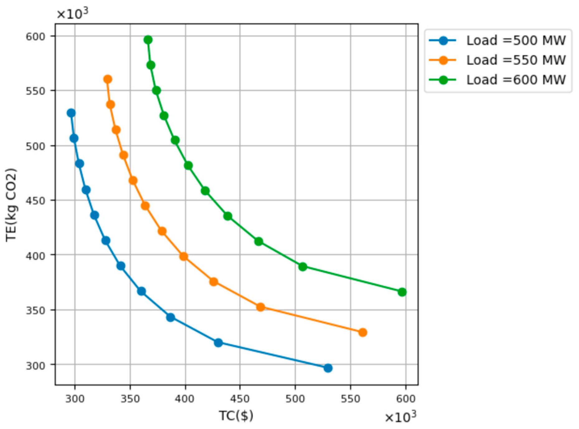
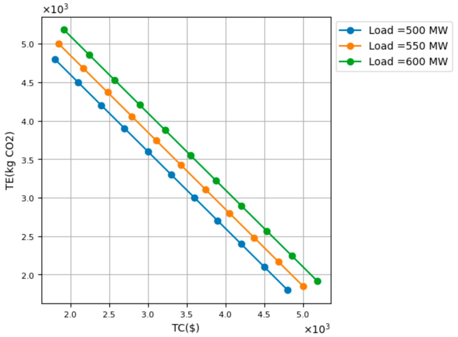
We assume a sufficient number of values for ranging between ( and ( that have been found above. In total, we assume 11 values, which is sufficient to obtain the Pareto optimal frontier while retaining the solution times within a reasonable range. This results in 11 pairs for the total emissions and the total cost, which form the Pareto frontier (for example, see Figure 1 below, where every Pareto frontier has 11 dots).

Figure 1.
Set of solutions for total emissions (TE) and total operational cost (TC) corresponding to sensitivity study S1.
In summary, for every sensitivity study (S1–S8), three levels of demand are assumed (500 MW, 550 MW, and 600 MW) and for every level of demand, a total of 13 optimization problems are solved as described above; the first two are solved in order to obtain minimum and maximum values for the total cost and emissions, i.e., , , and . These values are then used to determine 11 bounds on total emissions, , as in (14), for each of which an optimization model is solved as described above.
Therefore, optimization problems are solved for every sensitivity study. In total, optimization problems are solved for all 8 sensitivity studies. The corresponding solution time for solving all 312 problems is approximately 48 h, and is mostly affected by the nonlinear objective functions and constraints, i.e., Equations (1)–(6).
Section 6 below discusses the results of the sensitivity analyses.
6. Discussion
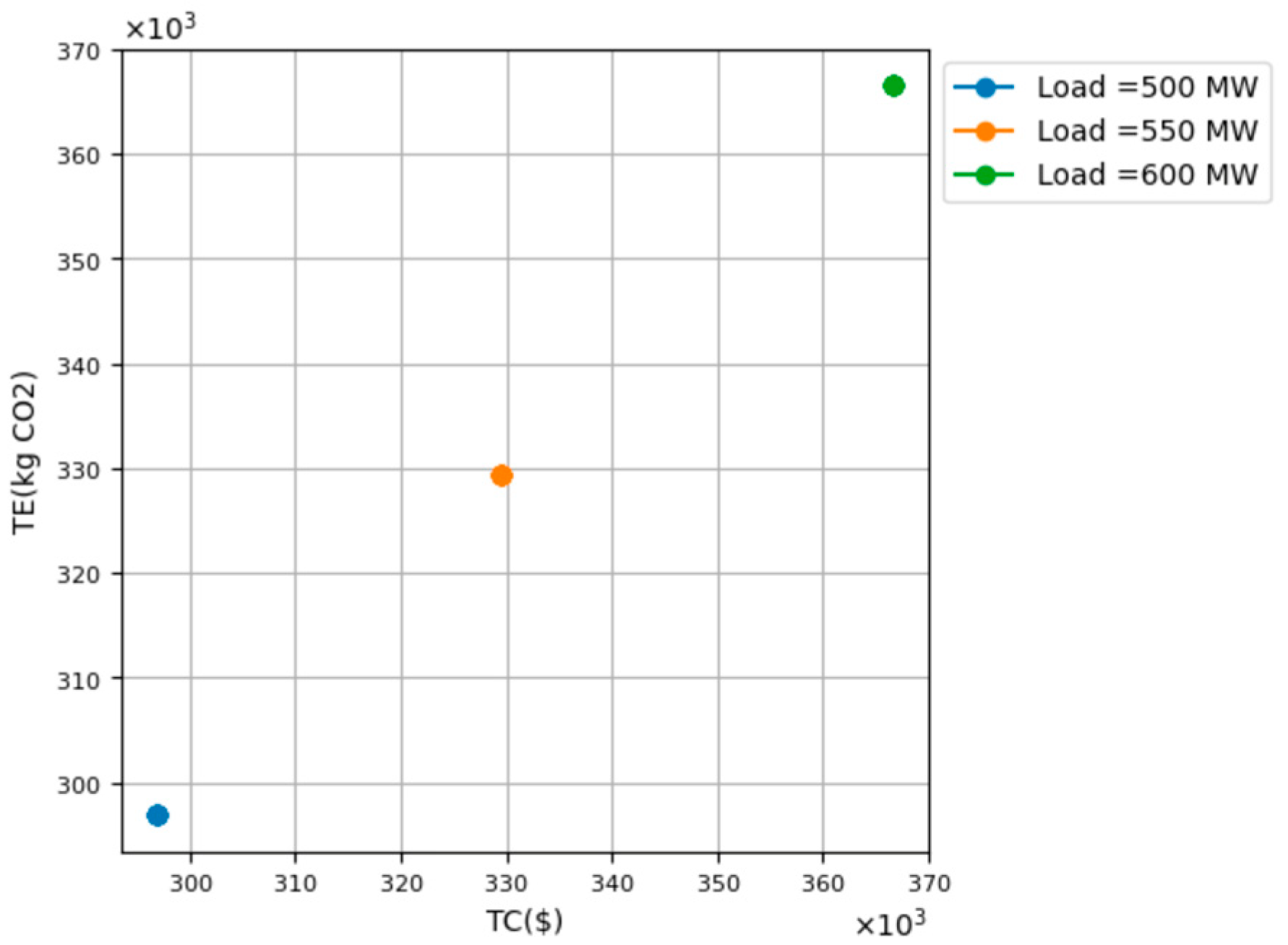
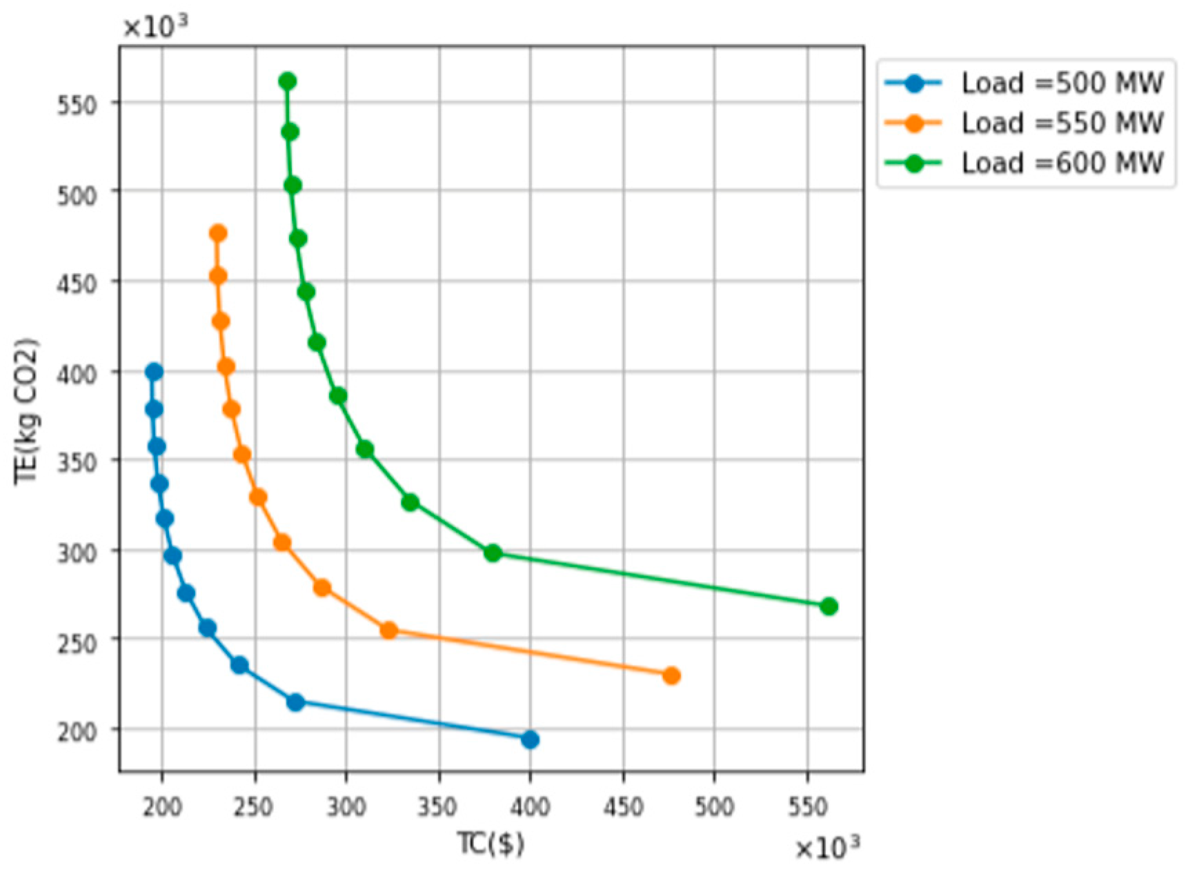
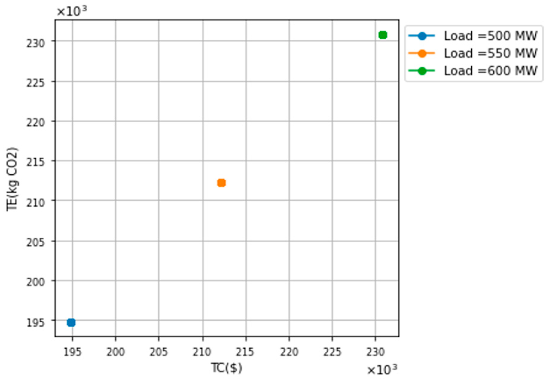
The results are presented in Figure 1, Figure 2, Figure 3, Figure 4, Figure 5, Figure 6, Figure 7 and Figure 8 below, which correspond to sensitivity studies S1–S8.
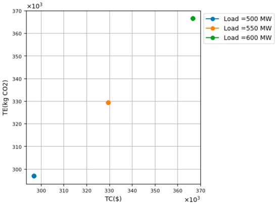
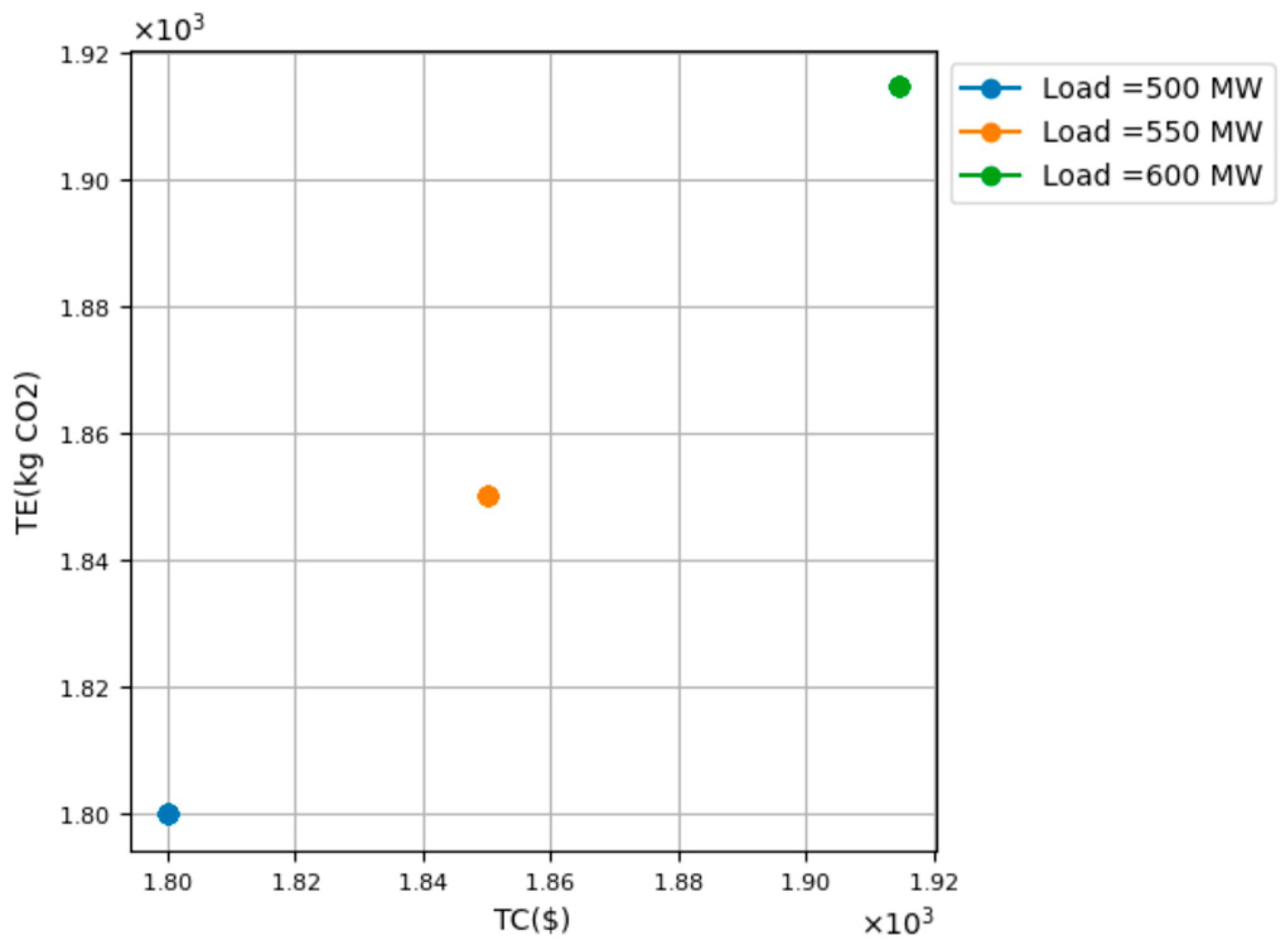
Figure 2.
Set of solutions for total emissions (TE) and total operational cost (TC) corresponding to sensitivity study S2.
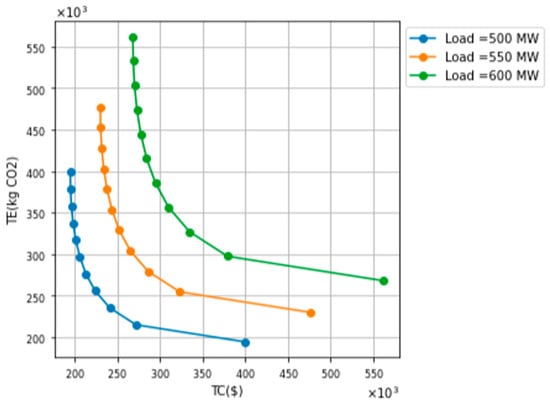
Figure 3.
Set of solutions for total emissions (TE) and total operational cost (TC) corresponding to sensitivity study S3.
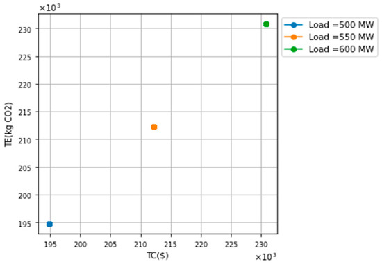
Figure 4.
Set of solutions for total emissions (TE) and total operational cost (TC) corresponding to sensitivity study S4.
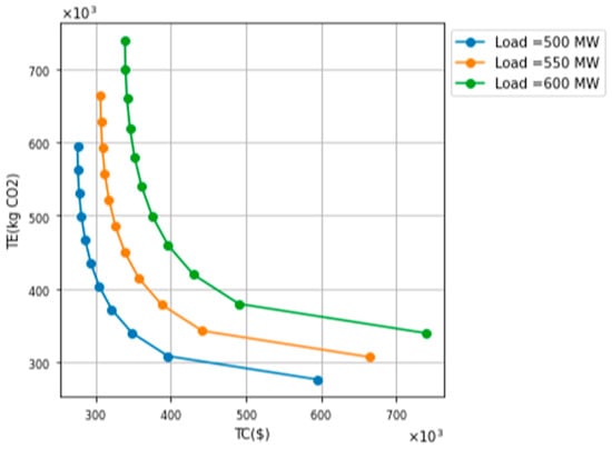
Figure 5.
Set of solutions for total emissions (TE) and total operational cost (TC) corresponding to sensitivity study S5.

Figure 6.
Set of solutions for total emissions (TE) and total operational cost (TC) corresponding to sensitivity study S6.

Figure 7.
Set of solutions for total emissions (TE) and total operational cost (TC) corresponding to sensitivity study S7.
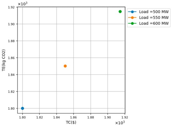
Figure 8.
Set of solutions for total emissions (TE) and total operational cost (TC) corresponding to sensitivity study S8.
In all figures, it can be observed that as the demand increases (500 MW -> 550 MW -> 600 MW), the corresponding set of optimal solutions is shifted to higher values for both total emissions (TE) and total operational cost (TC), i.e., they are shifted towards the upper-right part of the figure. This is explained by the fact that greater levels of demand require greater generation of power or heat, and result in a greater level of emissions.
Notice also that for sensitivity studies S1, S3, and S5, a Pareto frontier is obtained as opposed to studies S2, S4 and S6, where the set of solutions is essentially concentrated on one point, each for a level of demand. This has been explained in Table 1 and Table 2 above, i.e., it happens because for studies S1, S3 and S5, the generation units are characterized by an inverse relationship between total emissions and total costs, meaning that the units that are expensive to yield low emissions, whereas the units that are inexpensive to yield a high amount of emissions. In such an energy system, achieving lower levels of total emissions (i.e., moving downwards on the vertical axis) inevitably leads to an increase in total costs (i.e., a rightwards movement on the horizontal axis). And vice versa, achieving lower total costs will inevitably lead to an increase in the resulting CO2 emissions. Therefore, there is a tradeoff according to which it is not possible to improve both objectives of minimizing the cost and the CO2 emissions at the same time.
On the other hand, in studies S2, S4 and S6 the relationship between the cost and emission coefficients is direct (see Table 1 and Table 2), meaning that the units that are characterized by high (or low) cost coefficients are also characterized by high (or low) emission coefficients. In this case, the optimal solution is always to select the most economic units; these are also units that emit the smallest amount of kg CO2, thereby leading to the solution space concentrated in one point.
Notice that the inclusion of CHP units does not affect the shape of the Pareto frontier. By comparing Figure 1, where CHP units are not included, with Figure 3 and Figure 5, where CHP units are included, we observe that the only effect of the CHP units on the Pareto frontier is that there are points where it is less linear, and this is because of the extra nonlinearities added to the optimization models through the inclusion of Constraints (3) and (6) that have significant nonlinear elements.
Regarding Figure 7 and Figure 8 below, these correspond to studies S7 and S8, respectively. In Figure 7, it can be observed that the Pareto optimal frontier is no longer nonlinear but has a straight line. This is because in this case, both objective functions (cost minimization and emission minimization) are linear since the coefficients of the quadratic terms are both zero. For this reason, the resulting Pareto frontier has a linear shape as opposed to cases S1, S3 and S5 above, where the frontier has a nonlinear shape since the coefficients of the quadratic terms are both non-zero.
Figure 8 shows that the solution collapses into three points, each corresponding to the three different levels of demand, for the same reasons that apply to the nonlinear cases above (e.g., see study S2). It can therefore be seen that the type of the function (linear/nonlinear) for the operational cost and emissions has no effect when there is a direct relationship between the coefficients of the higher-order terms for cost and emissions.
Below, we illustrate the proposed framework of the Pareto frontier sensitivity analysis. This depiction, consisting of six steps, validates the methodology presented above. Specifically, the process consists of the following components.
- Define Objectives:
- ◦
- Objectives: Definition of the objectives of minimizing operational costs and CO2 emissions.
- ◦
- Inputs: List of the technoeconomic characteristics of generation units and the types of objective functions for operational cost and emissions. These become inputs.
- Formulate the Problem:
- ◦
- Mathematical Formulation: Definition of the equations representing the cost and emissions for thermal, heat-only, and CHP units.
- ◦
- Constraints: Definition of the constraints on power and heat outputs, as well as balance equations for meeting electricity and heat demand.
- Perform Optimization:
- ◦
- Step 1: Minimize total operational cost subject to constraints. Output: TCmin and corresponding emissions.
- ◦
- Step 2: Minimize total emissions subject to constraints. Output: TEmin and corresponding cost.
- Generate Pareto Frontier:
- ◦
- Intermediate Step: Define a range of emission limits (ElimE) between TEmin and TEmax.
- ◦
- Step 3: Minimize total cost for each Elim to find corresponding TC. This step is repeated for multiple values of Elim.
- Sensitivity Analysis:
- ◦
- Case Studies: Conduct different case studies with varying input parameters (cost coefficients, emissions coefficients, generation unit types).
- ◦
- Result Analysis: Plot and analyze the Pareto frontiers for each case study to identify the trade-offs and dependencies.
- Conclusion and Insights:
- ◦
- Result Interpretation: Discuss how variations in parameters affect the Pareto frontier.
- ◦
- Policy Implications: Provide insights for policymakers and stakeholders based on the analysis.
Section 7 below presents remarks on future work pathways and concludes the manuscript.
7. Conclusions and Future Work
The current paper presents sensitivity analyses on the Pareto frontier for energy systems of various types of generation technologies (thermal power stations, heat-only units and CHP units), types of mathematical functions for the operational cost and for the CO2 emissions (quadratic versus linear), and for different technoeconomical characteristics of the generation units. These studies contribute to a growing body of literature that seeks to harmonize economic considerations with environmental imperatives in energy. This research underlines the critical dependencies within the energy system’s operational framework, highlighting the complex interplay between environmental impact and economic feasibility. The insights drawn from this analysis are intended to guide future research and policy formulation in the pursuit of an optimized, balanced, and sustainable energy future.
Future work in this area includes conducting Pareto sensitivity analyses for power systems with portfolios of Smart Grid Technologies [23] such as Energy Storage [24,25], Dynamic Line Rating systems [26], Demand Response schemes [27], Coordinated Voltage Control Automation [28] and Soft Open Points [29,30,31], as well as Smart Electric Vehicle charging technologies such as Vehicle to Grid (V2G) and Vehicle to Building (V2B) [32,33,34,35]. In addition, it is of interest to the authors to utilize novel methodologies for carrying out Pareto frontier analyses such as the Backwards Induction methodology [36], and Deep Neural Networks [37], among others. In addition, part of future work also involves considering various types of uncertainty including decision-dependent sources and exogenous uncertainty [38,39] and incorporating sources of uncertainty in the analysis using Robust Optimization, Stochastic Optimization or Real Options frameworks [40].
Author Contributions
Methodology, S.G., X.Z. and T.Z.; Validation, and G.S.; Formal analysis, S.G.; Investigation, X.Z.; Data curation, X.Z. and T.Z.; Writing—original draft, S.G.; Visualization, and G.S.; Supervision, and G.S. All authors have read and agreed to the published version of the manuscript.
Funding
This research received no external funding.
Institutional Review Board Statement
Not applicable.
Informed Consent Statement
Not applicable.
Data Availability Statement
Data are contained within the article.
Conflicts of Interest
The authors declare no conflict of interest.
Nomenclature
| Abbreviations | |
| Combined Heat and Power | |
| Carbon dioxide | |
| Input Parameters and sets | |
| Set of thermal units | |
| Set of heat-only units | |
| Set of CHP units | |
| ) in the quadratic term of the objective function for thermal unit i | |
| ) | |
| ) | |
| ) in the quadratic term of the objective function for CO2 emissions for thermal unit i | |
| ) in the first order term of the objective function for thermal unit i | |
| ) in the first order term of the objective function for CO2 emissions for thermal unit i | |
| Constant ) in the objective function for CO2 emissions for thermal unit i | |
| ) in the quadratic term of the objective function for CO2 emissions for heat-only unit i | |
| ) in the first order term of the objective function for CO2 emissions for heat-only unit i | |
| Constant ) in the objective function for CO2 emissions for heat-only unit i | |
| ) of the objective function for thermal unit i | |
| ) in the quadratic term of the objective function for heat-only unit i | |
| ) in the first order term of the objective function for heat-only unit i | |
| ) of the objective function for heat-only unit i | |
| ) in the quadratic term of the objective function for CHP unit i | |
| ) in the quadratic term of the objective function for CHP unit i | |
| ) in the quadratic term of the objective function, representing the interdependency between electricity and heat output for CHP unit i | |
| ) in the first order term of the objective function for heat-only unit i | |
| ) in the first order term of the objective function for heat-only unit i | |
| ) of the objective function for heat-only unit i | |
| ) in the quadratic term of the objective function for CO2 emissions for CHP unit i | |
| ) in the quadratic term of the objective function for CO2 emissions for CHP unit i | |
| ) in the quadratic term of the objective function for CO2 emissions for CHP unit i | |
| ) in the first order term of the objective function for CHP unit i | |
| ) in the first order term of the objective function for CHP unit i | |
| ) of thermal unit i | |
| ) of thermal unit i | |
| Lower bound for the heat-output () of heat-only unit i | |
| ) of heat-only unit i | |
| Decision Variables | |
| Total operational cost (USD) | |
| Total CO2 emissions (kg) | |
| Cost of generating electricity (USD) from all thermal units | |
| Cost of generating heat (USD) from all heat-only units | |
| Cost of generating heat and electricity (USD) from all CHP units | |
| Total CO2 emissions (kg CO2) from generating electricity from all thermal units | |
| Total CO2 emissions (kg CO2) from generating heat from all heat-only units | |
| Total CO2 emissions (kg CO2) from generating heat and power from all CHP units | |
| Heat output (MW) of heat-only unit | |
| Heat output (MW) of CHP unit | |
References
- Kuroda, K.; Magori, H.; Ichimura, T.; Yokoyama, R. A hybrid multi-objective optimization method considering optimization problems in power distribution systems. J. Mod. Power Syst. Clean Energy 2015, 3, 41–50. [Google Scholar] [CrossRef]
- Pandya, S.B.; Ravichandran, S.; Manoharan, P.; Jangir, P.; Alhelou, H.H. Multi-objective optimization framework for optimal power flow problem of hybrid power systems considering security constraints. IEEE Access 2022, 10, 103509–103528. [Google Scholar] [CrossRef]
- Zhang, M.; Li, Y. Multi-objective optimal reactive power dispatch of power systems by combining classification-based multi-objective evolutionary algorithm and integrated decision making. IEEE Access 2020, 8, 38198–38209. [Google Scholar] [CrossRef]
- Jackson, D.; Belakaria, S.; Cao, Y.; Doppa, J.R.; Lu, X. Machine learning enabled fast multi-objective optimization for electrified aviation power system design. In Proceedings of the 2020 IEEE Energy Conversion Congress and Exposition (ECCE), Detroit, MI, USA, 11–15 October 2020; pp. 6385–6390. [Google Scholar] [CrossRef]
- Wei, F.; Yang, G.; Yang, D. A multi-objective optimization approach for photovoltaic and battery sizing in an off-grid power system. In Proceedings of the 2023 International Conference on Smart Electrical Grid and Renewable Energy (SEGRE), Changsha, China, 16–19 June 2023; pp. 373–379. [Google Scholar] [CrossRef]
- Zhang, Y.; Zhang, C.; Wu, T.; Zhong, X.; Wei, X.; Wang, G.; An, J.; Zhu, J. Mutli-objective optimized operation of integrated energy system with solar and wind renewables. In Proceedings of the 2020 IEEE/IAS Industrial and Commercial Power System Asia (I&CPS Asia), Weihai, China, 13–16 July 2020; pp. 206–212. [Google Scholar] [CrossRef]
- Mohamad, F.; Teh, J.; Abunima, H. Multi-objective optimization of solar/wind penetration in power generation systems. IEEE Access 2019, 7, 169094–169106. [Google Scholar] [CrossRef]
- Martins, P.E.T.; Oleskovicz, M. Multi-objective optimization aiming to minimize the number of power quality monitors and multiple fault estimations in unbalanced power distribution systems. IEEE Trans. Power Deliv. 2022, 37, 1315–1323. [Google Scholar] [CrossRef]
- Zheng, K.; Wang, Y.; Chen, Q.; Lu, D. Multi-objective power network partition: Finding the pareto frontier. In Proceedings of the 2019 IEEE Power & Energy Society General Meeting (PESGM), Atlanta, GA, USA, 4–8 August 2019; pp. 1–5. [Google Scholar] [CrossRef]
- Zhang, C.; Chen, H.; Xu, X.; Cai, R. Pareto front of multi-objective optimal reactive power dispatch. In Proceedings of the 2014 IEEE PES Asia-Pacific Power and Energy Engineering Conference (APPEEC), Hong Kong, China, 7–10 December 2014; pp. 1–6. [Google Scholar] [CrossRef]
- Li, Y.; Hu, J.; Zeng, W. Optimal scheduling of distributed photovoltaic power using pareto frontier principle. In Proceedings of the 2022 IEEE 5th International Conference on Electronics Technology (ICET), Chengdu, China, 13–16 May 2022; pp. 635–639. [Google Scholar] [CrossRef]
- Mu, C.; Wang, K.; Ni, Z.; Sun, C. Cooperative differential game-based optimal control and its application to power systems. IEEE Trans. Ind. Inform. 2020, 16, 5169–5179. [Google Scholar] [CrossRef]
- Asrari, A.; Lotfifard, S.; Payam, M.S. Pareto dominance-based multiobjective optimization method for distribution network reconfiguration. IEEE Trans. Smart Grid 2016, 7, 1401–1410. [Google Scholar] [CrossRef]
- Abido, M.A. Multiobjective optimal power flow using strength Pareto evolutionary algorithm. In Proceedings of the 39th International Universities Power Engineering Conference, Bristol, UK, 6–8 September 2004; Volume 1, pp. 457–461. [Google Scholar]
- Luo, Y.; Yuan, H.; Hu, Z.; Yang, D.; Zhang, H. Optimal scheduling of micro-energy grid based on paretof frontier under uncertainty and pollutant emissions. IEEE Trans. Smart Grid 2024, 15, 368–380. [Google Scholar] [CrossRef]
- Xia, M.; Zhou, Q.; Sykulski, J.; Yang, S.; Ma, Y. A multi-objective topology optimization methodology based on pareto optimal min-cut. IEEE Trans. Magn. 2020, 56, 7510505. [Google Scholar] [CrossRef]
- Nie, P.; Wang, G.; Wang, Y. Necessary and sufficient conditions for pareto optimal solution of backward stochastic system with application. IEEE Trans. Autom. Control 2023, 68, 6696–6710. [Google Scholar] [CrossRef]
- Moghadasi, A.H.; Heydari, H.; Farhadi, M. Pareto optimality for the design of SMES solenoid coils verified by magnetic field analysis. IEEE Trans. Appl. Supercond. 2011, 21, 13–20. [Google Scholar] [CrossRef]
- Baumgartner, U.; Magele, C.; Renhart, W. Pareto optimality and particle swarm optimization. IEEE Trans. Magn. 2004, 40, 1172–1175. [Google Scholar] [CrossRef]
- Bosshard, R.; Kolar, J.W.; Mühlethaler, J.; Stevanović, I.; Wunsch, B.; Canales, F. Modeling and η—α-pareto optimization of inductive power transfer coils for electric vehicles. IEEE J. Emerg. Sel. Top. Power Electron. 2015, 3, 50–64. [Google Scholar] [CrossRef]
- Strbac, G.; Kirschen, D. Fundamentals of Power System Economics; John Wiley & Sons, Ltd.: Hoboken, NJ, USA, 2004. [Google Scholar]
- Guo, T.; Henwood, M.I.; van Ooijen, M. An algorithm for combined heat and power economic dispatch. IEEE Trans. Power Syst. 1996, 11, 1778–1784. [Google Scholar] [CrossRef]
- Giannelos, S.; Borozan, S.; Aunedi, M.; Zhang, X.; Ameli, H.; Pudjianto, D.; Konstantelos, I.; Strbac, G. Modelling smart grid technologies in optimisation problems for electricity grids. Energies 2023, 16, 5088. [Google Scholar] [CrossRef]
- Giannelos, S.; Djapic, P.; Pudjianto, D.; Strbac, G. Quantification of the energy storage contribution to security of supply through the F-Factor methodology. Energies 2020, 13, 826. [Google Scholar] [CrossRef]
- Giannelos, S.; Jain, A.; Borozan, S.; Falugi, P.; Moreira, A.; Bhakar, R.; Mathur, J.; Strbac, G. Long-term expansion planning of the transmission network in India under multi-dimensional uncertainty. Energies 2021, 14, 7813. [Google Scholar] [CrossRef]
- Giannelos, S.; Konstantelos, I.; Strbac, G. Option value of dynamic line rating and storage. In Proceedings of the 2018 IEEE International Energy Conference (ENERGYCON), Limassol, Cyprus, 3–7 June 2018; pp. 1–6. [Google Scholar] [CrossRef]
- Giannelos, S.; Konstantelos, I.; Strbac, G. Option value of demand-side response schemes under decision-dependent uncertainty. IEEE Trans. Power Syst. 2018, 33, 5103–5113. [Google Scholar] [CrossRef]
- Konstantelos, I.; Giannelos, S.; Strbac, G. Strategic valuation of smart grid technology options in distribution networks. IEEE Trans. Power Syst. 2017, 32, 1293–1303. [Google Scholar] [CrossRef]
- Giannelos, S.; Konstantelos, I.; Strbac, G. Investment model for cost-effective integration of solar PV capacity under uncertainty using a portfolio of energy storage and soft open points. In Proceedings of the IEEE Milan PowerTech, Milan, Italy, 23–27 June 2019; pp. 1–6. [Google Scholar] [CrossRef]
- Giannelos, S.; Konstantelos, I.; Strbac, G. Option value of soft open points in distribution networks. In Proceedings of the IEEE Eindhoven PowerTech, Eindhoven, The Netherlands, 29 June–2 July 2015; pp. 1–6. [Google Scholar] [CrossRef]
- Giannelos, S.; Konstantelos, I.; Strbac, G. Stochastic optimisation-based valuation of smart grid options under firm DG contracts. In Proceedings of the 2016 IEEE International Energy Conference (ENERGYCON), Leuven, Belgium, 4–8 April 2016; pp. 1–7. [Google Scholar] [CrossRef]
- Borozan, S.; Giannelos, S.; Aunedi, M.; Strbac, G. Option value of EV smart charging concepts in transmission expansion planning under uncertainty. In Proceedings of the IEEE 21st Mediterranean Electrotechnical Conference (MELECON), Palermo, Italy, 14–16 June 2022; pp. 63–68. [Google Scholar] [CrossRef]
- Giannelos, S.; Borozan, S.; Moreira, A.; Strbac, G. Techno-economic analysis of smart EV charging for expansion planning under uncertainty. In Proceedings of the IEEE Belgrade PowerTech, Belgrade, Serbia, 25–29 June 2023; pp. 1–7. [Google Scholar] [CrossRef]
- Borozan, S.; Giannelos, S.; Strbac, G. Strategic network expansion planning with electric vehicle smart charging concepts as investment options. Adv. Appl. Energy 2022, 5, 100077. [Google Scholar] [CrossRef]
- Giannelos, S.; Bellizio, F.; Strbac, G.; Zhang, T. Machine learning approaches for predictions of CO2 emissions in the building sector. Electr. Power Syst. Res. 2024, 235, 110735. [Google Scholar] [CrossRef]
- Giannelos, S.; Borozan, S.; Strbac, G.A. Backwards induction framework for quantifying the option value of smart charging of electric vehicles and the risk of stranded assets under uncertainty. Energies 2022, 15, 3334. [Google Scholar] [CrossRef]
- Giannelos, S.; Moreira, A.; Papadaskalopoulos, D.; Borozan, S.; Pudjianto, D.; Konstantelos, I.; Sun, M.; Strbac, G. A machine learning approach for generating and evaluating forecasts on the environmental impact of the buildings sector. Energies 2023, 16, 2915. [Google Scholar] [CrossRef]
- Giannelos, S.; Konstantelos, I.; Strbac, G. Endogenously stochastic demand side response participation on transmission system level. In Proceedings of the IEEE International Energy Conference (ENERGYCON), Limassol, Cyprus, 3–7 June 2018; pp. 1–6. [Google Scholar] [CrossRef]
- Giannelos, S.; Konstantelos, I.; Strbac, G. A new class of planning models for option valuation of storage technologies under decision-dependent innovation uncertainty. In Proceedings of the IEEE Manchester PowerTech, Manchester, UK, 18–22 June 2017; pp. 1–6. [Google Scholar] [CrossRef]
- Buurman, J.; Babovic, V. Adaptation pathways and real options analysis: An approach to deep uncertainty in climate change adaptation policies. Policy Soc. 2016, 35, 137–150. [Google Scholar] [CrossRef]
Disclaimer/Publisher’s Note: The statements, opinions and data contained in all publications are solely those of the individual author(s) and contributor(s) and not of MDPI and/or the editor(s). MDPI and/or the editor(s) disclaim responsibility for any injury to people or property resulting from any ideas, methods, instructions or products referred to in the content. |
© 2024 by the authors. Licensee MDPI, Basel, Switzerland. This article is an open access article distributed under the terms and conditions of the Creative Commons Attribution (CC BY) license (https://creativecommons.org/licenses/by/4.0/).

