Abstract
Sustainable manufacturing practices are crucial in job shop scheduling (JSS) to enhance the resilience of production systems against resource shortages and regulatory changes, contributing to long-term operational stability and environmental care. JSS involves rapidly changing conditions and unforeseen disruptions that can lead to inefficient resource use and increased waste. However, by addressing these uncertainties, we can promote more sustainable operations. Reinforcement learning-based job shop scheduler agents learn through trial and error by receiving scheduling decisions feedback in the form of a reward function (e.g., maximizing machines working time) from the environment, with their primary challenge being the handling of dynamic reward functions and navigating uncertain environments. Recently, Reward Machines (RMs) have been introduced to specify and expose reward function structures through a finite-state machine. With RMs, it is possible to define multiple reward functions for different states and switch between them dynamically. RMs can be extended to incorporate domain-specific prior knowledge, such as task-specific objectives. However, designing RMs becomes cumbersome as task complexity increases and agents must react to unforeseen events in dynamic and partially observable environments. Our proposed Ontology-based Adaptive Reward Machine (ONTOADAPT-REWARD) model addresses these challenges by dynamically creating and modifying RMs based on domain ontologies. This adaptability allows the model to outperform a state-of-the-art baseline algorithm in resource utilization, processed orders, average waiting time, and failed orders, highlighting its potential for sustainable manufacturing by optimizing resource usage and reducing idle times.
1. Introduction
Nowadays, energy consumption has become an important issue due to its significant environmental impact, attracting much attention. According to studies [1], China’s and India’s current energy consumption will double by 2040. The industrial sector accounted for 37% of global energy use in 2022, resulting in the emission of 9.0 Gt (Gigatonne) of CO2, which constitutes a quarter of total CO2 emissions from the global energy system [2]. Thus, manufacturing enterprises urgently need sustainable practices to achieve economic, ecological, and social goals. For instance, Ref. [3] proposed a low-carbon scheduling model to optimize productivity and energy efficiency in job-shop environments, while Ref. [4] discussed the importance of sustainability assessment in manufacturing organizations. Additionally, Refs. [5,6] highlighted the use of advanced techniques such as multi-agent learning and smart manufacturing technologies to enhance sustainability. Job Shop Scheduling (JSS) plays a crucial role in manufacturing by optimizing production processes, ensuring efficient resource utilization, and meeting delivery deadlines. It helps to minimize production costs, reduce lead times, and improve overall productivity, ultimately contributing to the competitiveness and success of manufacturing operations. Effective JSS ensures that resources, such as machines, are allocated optimally to meet the manufacturing environment’s diverse and dynamic demands [7]. Effective job scheduling strategies have demonstrated the potential to decrease energy consumption and emissions through optimized production sequences, reduced idle times, and enhanced resource utilization [8,9]. They maximize resource utilization by intelligently allocating jobs to machines based on current workloads and machine availability, thereby reducing bottlenecks and idle times. This efficient allocation not only maximizes the use of available resources but also minimizes energy consumption and operational costs by ensuring that machines are operating at optimal capacity.
In dynamic and partially observable JSS environments, facing unforeseen situations is inevitable. For example, an urgent customer order with a tight deadline arrives suddenly, necessitating a reorganization of the current schedule to accommodate this priority job. Also, the observations made by the job shop scheduler agent are frequently derived from incomplete, ambiguous, and noisy data. For example, sensors tracking machine status could provide erroneous information about machine conditions. In such environments, the agent needs to be adaptive to emerging requirements or changes in the availability of the required resources. Reinforcement Learning (RL) methods [10,11,12] have gained attention for their adaptability to learning and optimizing schedules in dynamic scenarios. In RL, the agent learns optimal behavior through trial-and-error interactions with its environment, with the reward function, defined by the problem designer, serving as a crucial guide to incentivize desired actions while avoiding unintended outcomes. RL agents can continuously update schedules based on feedback from the environment. However, RL algorithms struggle with partial observability, as scheduling agents often operate with incomplete information about the factory’s state [13,14]. Furthermore, the complexity of the state space in JSS can hinder efficient exploration and learning, especially when unforeseen events introduce new states or transitions [15,16]. Specifying appropriate reward functions to guide scheduling decisions in the face of unforeseen events is challenging, and maintaining a balance between exploration and exploitation becomes intricate in the presence of uncertainty. Additionally, generalization from past experiences to novel, unexpected scenarios is challenging. Furthermore, integrating human expertise in the decision-making process adds further complexity to managing unforeseen events in JSS within an RL framework [17,18]. On the other hand, non-RL approaches often rely on various techniques such as heuristics, simulation, and optimization to address the challenges of unforeseen events. For instance, Ref. [19] proposed an adaptive scheduling algorithm for minimizing makespan in dynamic JSS, while Ref. [16] introduced a heuristic algorithm for similar problems. Additionally, Ref. [20] presented a linear programming-based method for JSS, and Ref. [21] suggested a dynamic scheduling approach based on a data-driven genetic algorithm. However, these approaches may struggle to effectively model and optimize for dynamic changes or unforeseen disruptions and variations (face of varying task duration, resource availability, and unexpected factors), as they often rely on static predefined strategies and lack the adaptability that RL techniques offer in response to evolving conditions. For example, traditional methods frequently utilize neighborhood-based approaches, genetic programming, and fuzzy logic, but these can be limited in handling dynamic JSS problems [22,23]. Moreover, despite advances in self-adaptive multi-objective algorithms, challenges remain in optimizing for both performance and sustainability under uncertain conditions [24,25].
Creating reward functions often demands domain expertise and can be time-consuming, leaving room for errors and limited coverage of all scenarios. Moreover, these functions struggle to generalize across different scheduling environments and cope with the inherent uncertainty present in JSS, such as unforeseen events. The literature proposes various techniques to handle these challenges. To provide more frequent feedback on appropriate behaviors, agents can be incentivized with intrinsic rewards [26]. Additionally, inner rewards can be generated using various reward shaping approaches, such as adaptive inner-reward shaping [27], bi-level optimization for shaping rewards [28], and context-sensitive reward shaping in multi-agent systems [29]. Dynamic reward shaping with user feedback is another effective method [30]. However, these techniques are challenging in dynamic and partially observable environments, especially when faced with unexpected events. Inverse reward design and reward learning from demonstration [31,32] infer the intents or goals of an expert demonstrating a task; however, these approaches only work when the agent has access to expert demonstrations.
Reward Machine (RM) is defined as a Finite-State Automata (FSA). It is a way to expose the reward function structure to the agent (i.e., the way it assigns rewards to different states and actions) to use it to decompose the problem and speed up learning [33]. The intuition is that the agent will be rewarded with different reward functions at different times, depending on the changes made in the RM. Partially observable and dynamic environments can present challenges for RM design, mainly when complex tasks and unexpected events occur [34]. Although various variations of RM have been proposed, such as learning RM in partially observable environments [35], hierarchies of RMs [36], and symbolic RMs [37], to define reward functions for complex tasks, they cannot still define reward functions adaptively and require manual reward assignment.
We address this gap by integrating ontology with RM, aiming to enhance the JSS and sustainability in manufacturing. Ontologies explicitly represent human knowledge about domains of interest and serve as critical components in knowledge management applications [38]. The hierarchical structure of ontologies, with subclasses inheriting the properties from their ascendant classes, facilitates inferring the environment’s properties. As the environment changes, new concepts (entities), properties, and relations may become apparent. Each concept can be associated with positive or negative properties, dependent on the domain being modeled by the ontology. Positive properties are desirable or valuable, whereas negative properties are undesirable or harmful or lead to negative outcomes. For example, in the domain of JSS, positive properties might represent a low order waiting time or high machine working time, while negative properties might represent a high machine idle time or high machine failure rate. In ontology, the properties are structured and related to other concepts within the domain, making it possible to reason about them and draw conclusions based on their relations. In our previous work [39], we introduced a new Ontology-based Adaptive Reward Function (OARF) method, which dynamically creates new reward functions using positive or negative properties to adapt the agent’s behavior based on the changing dynamics of the environment. The OARF method is extensively extended in this work by proposing an ONTOlogy-based ADAPTive REWARD Machine (ONTOADAPT-REWARD) model to dynamically/adaptively create/modify RMs. First, the RL agent models its observation as an ontology-based schema that maps low-level sensor data to high-level concepts, relations, and properties. This schema allows the agent to access the structure of ontological knowledge of the observation and to conduct logical reasoning based on this knowledge. Based on the new concepts and properties of the agent’s observation, the agent identifies unforeseen events by extracting subsumers and creating new transitions and reward functions for its RM. Finally, the agent can use multiple reinforcement learners for different reward functions.
The rest of this paper is organized as follows. Section 2 examines related works. Section 3 provides the required background information, and Section 4 describes JSS as a partially observable and dynamic environment. Section 5 describes our model and its different stages. In Section 6, the scenarios are defined, and the results are analyzed. Section 7 concludes with our findings and outlines future work.
2. Related Work
Static scheduling in JSS involves the creation of a fixed production schedule that remains unchanged throughout the manufacturing process. This approach assumes a stable and predictable manufacturing environment where all parameters are known in advance. Each job/order or operation is assigned to a specific machine and a predefined processing sequence based on factors like job priority, due dates, and setup times. Although static scheduling methods are relatively straightforward to implement and require less computational effort, they lack adaptability [40]. They need to account for real-time changes, such as machine breakdowns or shifts in job priorities, which can lead to suboptimal resource utilization and missed delivery deadlines. On the contrary, dynamic scheduling allows for real-time adjustments to the production schedule in response to changing conditions. It accommodates uncertainty and is well suited for modern manufacturing environments characterized by fluctuations in demand, machine failures, and evolving priorities. Dynamic scheduling systems continuously monitor the shop floor, collecting data on job progress, machine status, and unforeseen disruptions. Using this real-time information, dynamic scheduling algorithms can adapt the schedule to optimize resource utilization, minimize delays, and meet customer deadlines. This flexibility comes at the cost of increased complexity and computational requirements but it is essential for achieving agility and responsiveness in dynamic manufacturing settings [41,42]. Dynamic scheduling in job shops can be approached as an RL problem. The scheduler (agent) takes actions (schedule adjustments) to maximize a cumulative reward signal (e.g., minimizing production time, meeting deadlines) [15,43].
Adaptive reward functions are crucial in JSS due to the dynamic and complex nature of the environment. They allow scheduling algorithms to respond effectively to changing conditions, such as machine breakdowns or shifting job priorities, ensuring optimal scheduling decisions. Additionally, these functions enable the algorithm to balance multiple objectives, like minimizing production time and reducing costs, by dynamically adjusting the importance of each objective based on the current context, ultimately improving scheduling performance. Substantial efforts have been made to enrich the information in reward functions. RMs from [44] directly represent reward functions as FSAs. There have been efforts to learn the so-called perfect RM in [35] from the experience of an RL agent in a partially observable environment. They formulated finding a perfect RM problem as an optimization problem. Their method focuses on the RM that predicts what is possible and impossible in the environment at the abstract level. However, their method still needs to know a set of high-level propositional symbols and a labeling function that can detect them prior. So it does not work when there is unforeseen observation for which there is no experience in the training set. Learning Finite State Controllers (FSCs), [45] suggested looking for the smallest RM that correctly mimics the external reward signal given by the environment and whose optimal policy receives the most reward. It is a desirable property for RMs, but it requires computing optimal policies to compare their relative quality, which seems prohibitively expensive. With Deterministic Markov Models (DMMs), [46] proposed learning the RM that remembers sufficient information about history to make accurate predictions about the next observation. However, their approach needs to keep track of details that will not necessarily result in better predictions, especially in dynamic and noisy environments. In [36], the authors defined Hierarchies of RMs (HRMs), in which RM and its associated policies are reusable across several RMs. Ref. [37] proposed Symbolic RMs (SRMs) for incorporating high-level task knowledge when specifying the reward functions. It facilitates the expression of complex task scenarios and the specification of symbolic constraints. Ref. [37] developed a hierarchical Bayesian approach that can concretize an SRM by inferring appropriate reward assignments from expert demonstrations. Also, the Inverse Reward Design (IRD) proposed in [32] aims at inferring a reward function from an expert demonstration. However, these approaches only work when the agent can access expert demonstrations.
Knowledge-based RL seeks to guide agents in their exploration using prior knowledge. In [47], we proposed a new automatic goal generation model to evolve/generate new goals to address emerging requirements in unforeseen situations. However, a new goal could only be defined as returning the environment to a previous normal state. Also, we have proposed a new Ontology-based Adaptive Reward Function (OARF) method, which dynamically creates new reward functions based on domain ontologies [39]. However, we do not handle the design of RMs when dealing with increasingly complex tasks and unforeseen events in dynamic and partially observable environments. Reward shaping proposed by [48] added state-based potentials to the reward in each state. Exploration-driven approaches such as [26] incentivize agents with intrinsic rewards. Ref. [49] applied reward shaping approaches to multi-objective problems. However, it is not always apparent how general concepts describing intended behaviors can be translated into meaningful numeric rewards [50]. Ref. [27] proposed learning-based reward shaping to allow the agent to generate inner rewards to guide itself. However, their learning approach has challenges with a limited number of training steps and uncertain environments. Ref. [51] proposed a meta-learning framework to learn efficient reward shaping on newly sampled tasks automatically. However, they assumed that the state spaces of the task distribution are shared. Ref. [52] used genetic programming to find novel reward functions that improve learning system performance. Ref. [28] considered how to adaptively utilize a given parameterized shaping reward function, utilizing the beneficial part of the given shaping reward function as much as possible and meanwhile ignoring the non-beneficial shaping rewards. Ref. [29] described the use of context-aware potential functions in which different shaping functions should be used for different contexts to address different subgoals. However, the agent must autonomously learn the mapping from context to shaping function. Ref. [30] introduced a dynamic reward shaping approach in which a human provides verbal feedback translated into additional rewards. In [53], demonstrations from a teacher were used to shape a potential reward function by training a deep convolutional neural network. However, humans sometimes give the wrong reward, give feedback out of time, or the agent’s speech recognition system misinterprets the command.
3. Background
3.1. Markov Decision Process
By providing a discrete-time stochastic control process, a Markov Decision Process (MDP) can mathematically describe an environment in RL [54]. In the standard formulation of MDP , at time step , an agent is in state , takes an action , receives an immediate reward , and transitions to a next state . Let be a policy, where is the set of distributions over the action space . The discounted cumulative reward under policy is , where is a discount factor. The goal of RL is to find a policy that achieves the maximum cumulative reward . Under policy , the value function can be defined as the expected cumulative reward of an agent in a certain state s, . The action value function returns the expected cumulative reward for using action a in a certain state s, . Given a certain state s, the advantage function measures how much a certain action a is a good or bad decision, .
Partially Observable MDPs: In practice, most real-world problems are not fully captured by MDPs, and some are partially observable. A Partially Observable MDP (POMDP) has the following equation: [55]. POMDP has two extra components: the possibly infinite set of observations, and the function, which creates observations based on the unobservable state using a set of conditional observation probabilities. At each time, the agent receives an observation , with probability , that depends on the recently changed environment’s state and on the just taken action . Due to partial observability, learning is challenging in these circumstances since the same observation might be received from two separate states, each requiring a different optimal action.
3.2. Trust Region Policy Optimization
With a direct policy search within the specified policy class , where stands for the policy’s parameter space, it is possible to approximate optimal policy . We can update the parameter using policy gradient ascent, by computing , then updating with some learning rate . Another alternative would be to consider first a trust region optimization problem [54]:
for some . If we approximate the objective of the (1) linearly, , by correctly selecting given , we are able to recover the policy gradient update.
In this paper, the baseline algorithm uses Trust Region Policy Optimization (TRPO) [54] as its learning algorithm. TRPO captures the geometry of the parameter space influenced by the underlying distributions more effectively by employing information theoretic constraints rather than Euclidean constraints (as in (1)). Specifically, consider the following trust region formulation:
where the state visitation distribution induced by is denoted by . By enforcing the trust region with the KL divergence, the update in (2) optimizes a lower bound of during training to prevent making significant changes that irreversibly worsen policy performance as with the (1) for vanilla policy gradients.
3.3. Reward Machine
A Reward Machine (RM) [44] takes abstract descriptions of the environment as input and output reward functions. The assumption is that, according to the transitions made in the RM, the agent will be rewarded by various reward functions at various times. An RM sets several tasks for an RL agent in the environment and is defined over a collection of propositional symbols E that is related to a set of high-level events from the environment that the agent may detect using a labeling function . Given an environment experience , L assigns truth values to symbols in E, where is the observation observed after performing the action a when observing s. An RM is a tuple , where U is a finite set of states, is an initial state, is the state-transition function , and is the reward-transition function .
3.4. Ontology
Ontology [56] is utilized for semantic descriptions when needed (for instance, when an interpretation of an unanticipated or unforeseen event is needed). An ontology describes concepts C, properties F, and relations R. For example, the concept “Order” can be defined as an Order ⊑ Thing ⊓ ∃has.WaitingTime within the JSS ontology. It denotes that the concept “Order” is a Thing (that is, relation) and possesses the property “WaitingTime”. An ontology can represent all relations between concepts using a hierarchical approach, including conditional relations, multiple relations, and the inverse relations between successor and predecessor. The domain and range of a relation determine the concepts’ types and ranges. Instances are the “concrete things” represented by a concept; for example, “automobile repair” is an instance of the concept “Order”. To account for all the concept’s relations, we need to look at all (possibly complex) entailed descriptions of that concept. This is called subsumers [57]. Suppose that we have these relations {WaitingTime ⊑ Time, Order ⊑ Thing ⊓ ∃has.WaitingTime} in the ontology. Then, the subsumer for the concept Order will be {Thing, Time, ∃has.WaitingTime}.
4. Job Shop Scheduling: Partially Observable and Dynamic Environment
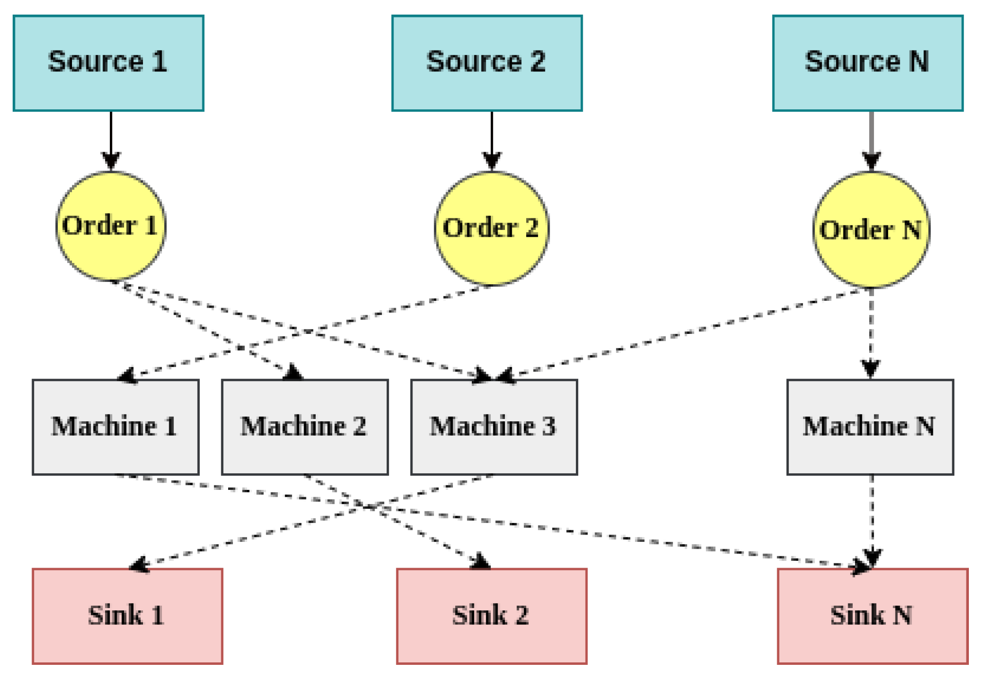
JSS refers to the problem of processing multiple orders on multiple machines, with several operational steps required for each order completed in a particular sequence. For example, the order might involve manufacturing consumer products such as automobiles. Figure 1 illustrates this environment. The JSS environment is selected to illustrate how our proposed model can work in real-world applications. Dynamism and partial observability are essential characteristics of the JSS environment. Unforeseen events like machine failures, extended processing times, or urgent orders can significantly impact the scheduling process [58,59].
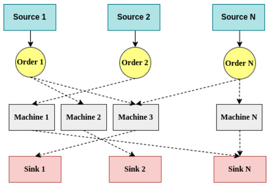
Figure 1.
Abstract view of the job shop scheduling environment. Dotted lines indicate possible operations.
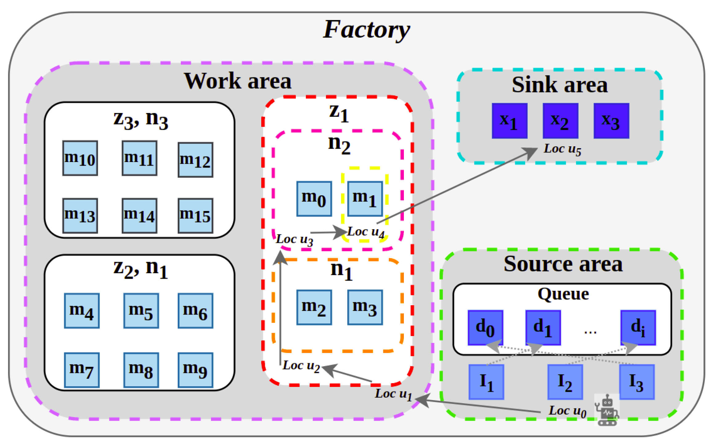
We have based our evaluation on a JSS environment (see Figure 2) using [60] with the following details.
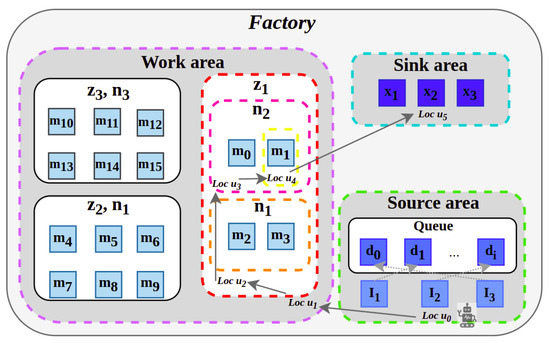
Figure 2.
Simulated job shop scheduling environment.
JSS Entities include the following:
- Orders should be processed by machines based on a specified sequence of operations.
- Sources , , and generate orders.
- Machines/Resources can process one order at a time. Machines are categorized into three groups: , , and . Each group consists of machines that can perform similar operations, following the Group Technology (GT) principle of forming part families based on process similarities. This grouping allows for streamlined processing of orders, as machines within the same group can be interchangeably used for specific types of operations, thereby reducing setup times and enhancing throughput.
- Work areas , , and are located in different locations in the factory to facilitate the efficient movement of orders. Each work area contains a subset of machine groups, ensuring that orders can be processed with minimal transportation delays between operations.
- Sinks , , and are entities that consume processed orders, and their capacity is the number of orders they consume at each time step.
- The scheduler agent selects an order and sends it to a machine/sink for its next operation step. The steps involved are as follows: The agent selects an order from the queue of orders at the source. Then, it moves to a work area and a group and selects a machine in the desired group to process the order. Finally, it selects an order from the queue of orders in the machine and places the processed order in a sink.
JSS Tasks: There are different tasks associated with every factory location that must be performed sequentially by the JSS agent. We assume our factory has six different locations and the tasks associated with each location are as follows:
- selects an order from the source order queue.
- selects a work area for moving the order there.
- selects a group for selecting a machine from it.
- selects a machine for processing the order.
- selects an order from the machine order queue to be processed.
- selects a sink to consume the processed order.
JSS Strategies: In the current implementation of JSS (the code of the baseline method and ONTOADAPT-REWARD-based proposed method is accessible to the public: https://github.com/akram0618/ontology-based-adaptive-reward-machine-RL (accessed on 1 January 2024)), the following strategies are used to complete the described tasks:
- Random strategy for tasks , , and , which selects a work area, group, or sink randomly;
- LIFO strategy for task , which selects the last order entered into the queue for resource allocation;
- FIFO strategy for task , which selects the first order entered into the queue for processing;
- RL strategy for task , which selects the machine with the highest reward.
Figure 2 illustrates the JSS environment. The factory is divided into three areas: sink, source, and work. When the JSS agent is located in each area, it can only observe the entities that are specifically located in that area. For example, in location , only , , and and their order queue are visible (i.e., the green dotted rectangle area). When the agent reaches the location , it can only observe work areas , , and (i.e., the purple dotted rectangle area), while at the location , it observes groups and (i.e., the red rectangle area). Location is where the agent can observe machines and (the pink dotted rectangle), whereas location is where it can observe only machine and its order queue (the yellow dotted rectangle). Finally, in location , the agent observes sinks , , and (i.e., the blue dotted rectangle area).
5. An Ontology-Based Adaptive Reward Machine for Reinforcement Learning Algorithms
In ONTOlogy-based ADAPTive REWARD Machine (ONTOADAPT-REWARD) model, firstly, the JSS agent models its state as an ontology-based schema. Next, based on the concepts and properties of the agent’s state, it extracts a relevant subsumer and labels its observation as a new propositional symbol. An ontology-based schema is also used to derive reward functions for each state (see ONTOADAPT-REWARD process in Figure 3 and the algorithmic procedure in Algorithm 1).
| Algorithm 1 Ontology-based Adaptive Reward Machine (ONTOADAPT-REWARD). |
|
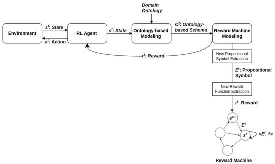
Figure 3.
Ontology-based Adaptive Reward Machine (ONTOADAPT-REWARD) model.
5.1. JSS Ontology
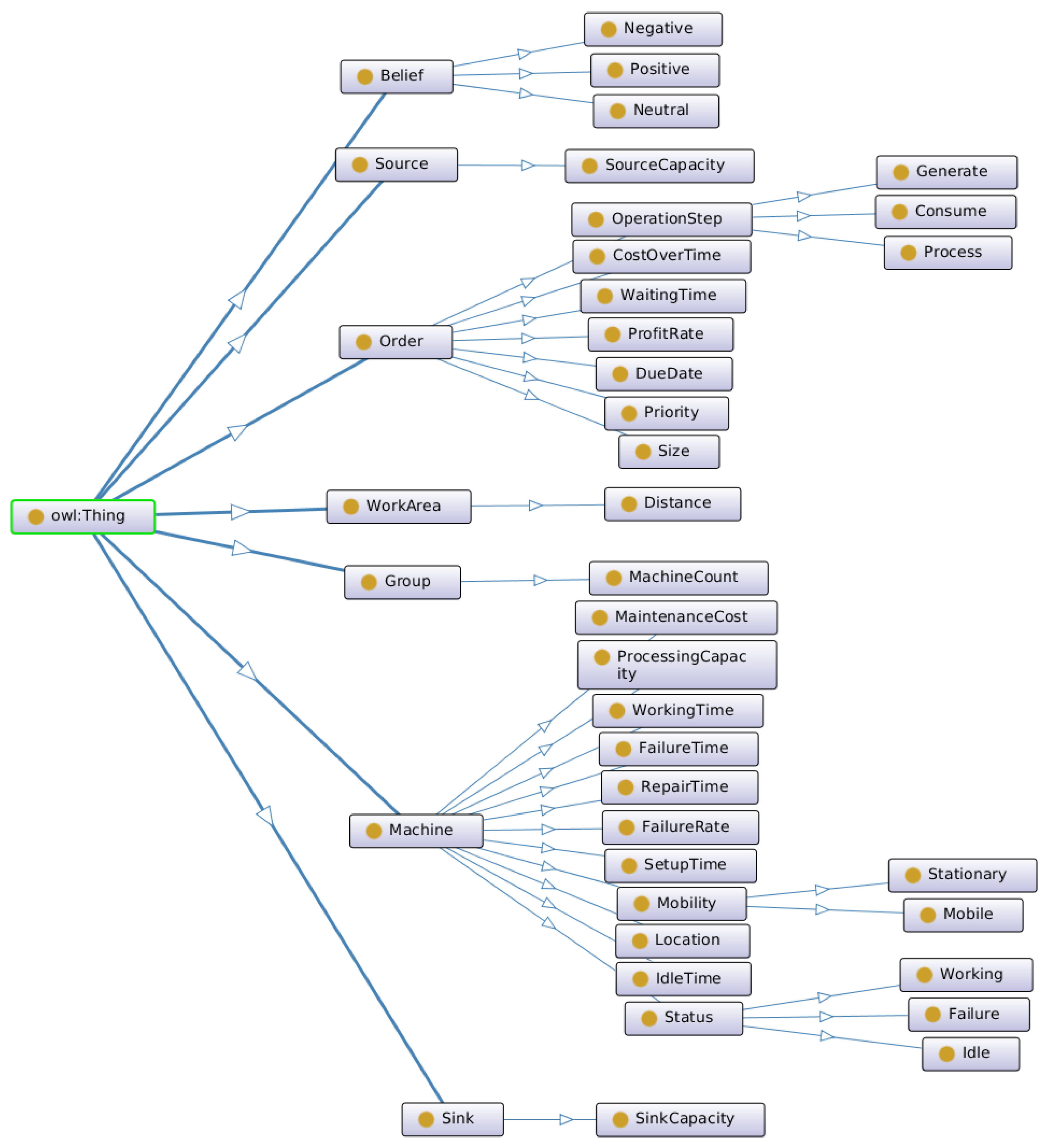
To represent the relevant concepts in the JSS environment, we use the ontology shown in Figure 4, with seven high-level concepts (i.e., superclass), including Belief, Source, Order, WorkArea, Group, Machine, and Sink, each associated with an individual entity defined within the JSS environment. A superclass can have subclasses shown by the “part of” relation. Subclasses can represent concepts more specific than those of a superclass. For example, Working, Failure, and Idle are part of Status, which is part of Machine. Belief is based on human experiences with concepts; for example, WorkingTime is associated with positive belief, and WaitingTime is associated with negative belief. It means that high waiting time has a negative impact on the agent’s performance.
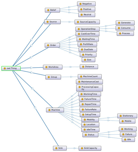
Figure 4.
Job shop scheduling environment ontology.
5.2. Modeling JSS as an RL Process
To define RMs for the JSS problem, we need to define actions, states, and reward functions for each task within the environment to formulate them as RL problems (see line 1 of Algorithm 1).
Actions: There are different action sets for different JSS tasks:
- , selecting one of the orders in the source order queue.
- , selecting one of the three work areas.
- , selecting one of the three groups of machines.
- , selecting one of the sixteen machines.
- , selecting one of the six orders in the machine order queue.
- , selecting one of the three sinks.
State: We represent the information of each state for the JSS agent at time step t using Equation (3). Specific parameters are detailed in Table 1.

Table 1.
State representation parameters.
The JSS agent’s state for different tasks is as follows:
- .
- .
- .
- .
- .
- .
Reward: The only predefined reward function is maximizing the average utilization rate of all the machines as depicted in Equation (4):
Because a failed machine cannot receive an order until it is repaired, the individual machine’s utilization percentage is calculated based on its working time as follows (where indicates the last utilization rate calculation time):
After that, the average utilization rate is calculated as follows:
Other reward functions will be extracted in Section 5.4.2 based on the proposed ONTOADAPT-REWARD model.
5.3. Ontology-Based Modeling of State
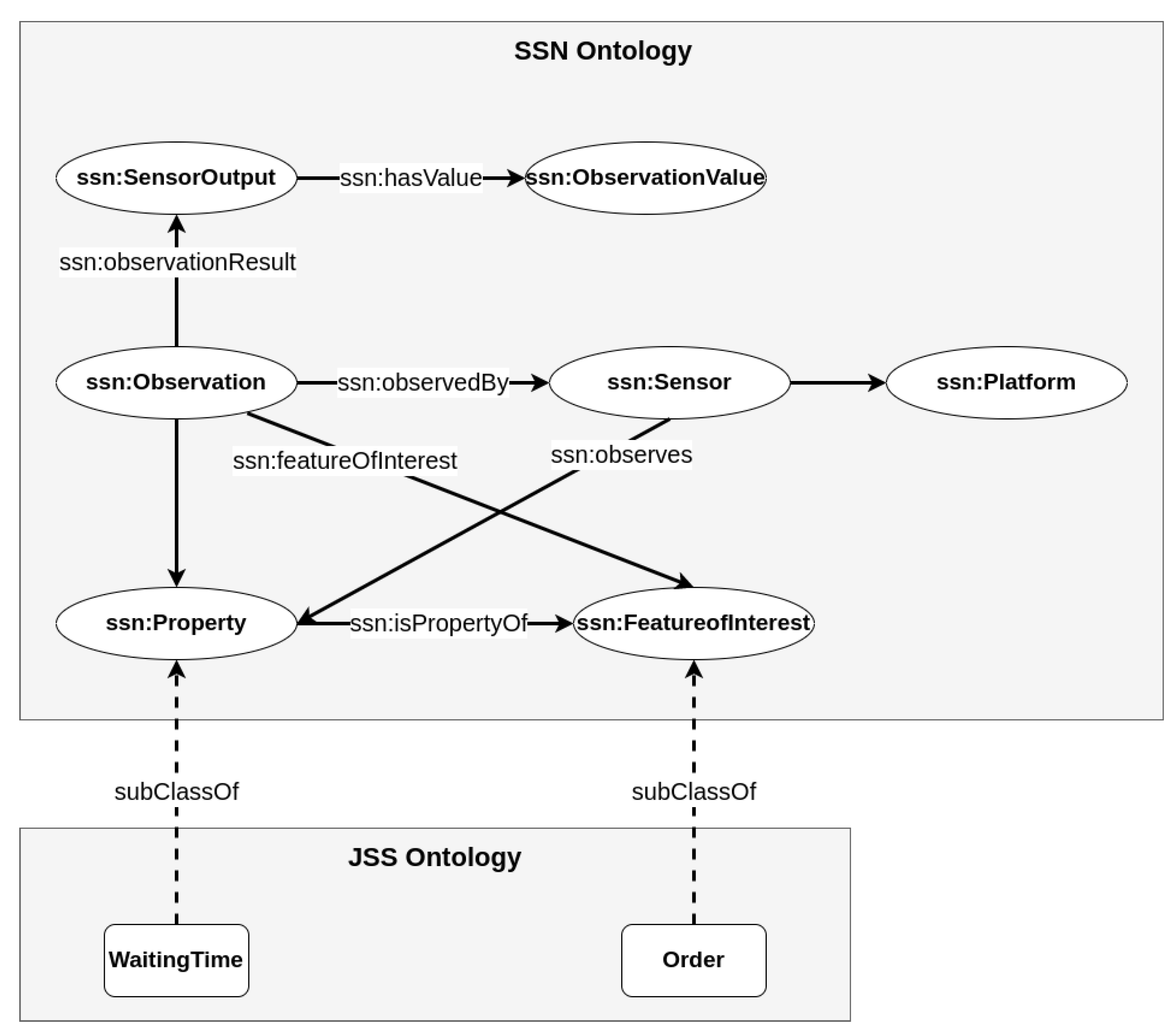
This paper uses ontology to allow agents to represent their observations within an ontological structure, mapping low-level sensor data streams to high-level concepts. Sensors typically produce raw, unstructured data streams that measure phenomena such as the waiting time of an order. Data collected by sensor resources are described by the Semantic Sensor Network (SSN) ontology, which is a model developed using a standard model of sensor networks [61]. Agents use the SSN ontology with cross-domain knowledge to annotate and present sensor data using the data model described in [62] (see Figure 5). Sensor data observed by an agent are described by the “ssn:Observation” class. The “ssn:Property” specifies the property (e.g., waiting time) of the feature of interest (e.g., order) that is described by the JSS ontology.
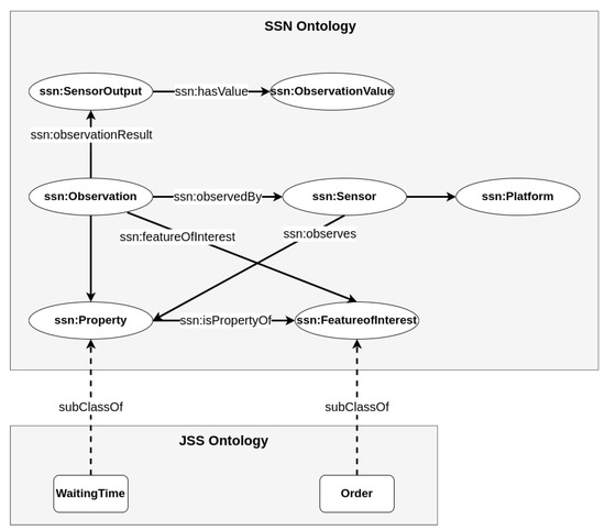
Figure 5.
Concept of the data model proposed in [62] to annotate and present sensor data.
In this paper, the RL agent annotates raw environment data streams using a semantic description defined by a combined ontology, where the environment data stream is indicated by concepts (e.g., machine and order) and their properties (e.g., working time and waiting time). This is referred to as an ontology-based schema (see line 3 of Algorithm 1). Based on this schema, we can access the ontological knowledge structure of the state and its ability to conduct logical reasoning.
We define as the schema that describes the data monitored/observed by the JSS agent at the time step t. C represents the set of concepts , F represents properties , and R represents the set of relations over these concepts, indicating how concepts and concepts/values are connected through properties (). For example, in an ontology-based schema for the JSS environment, the concept “Order” is defined as follows:
Order ⊑ Thing ⊓ ∃has.DueDate ⊓ ∃has.Priority ⊓ ∃has.WaitingTime ⊓ ∀has.OperationStep ⊓ ∃has.ProfitRate ⊓ ∀has.Size ⊓ ∃has.CostOverTime
This means the concept Order has different properties, including DueDate, Priority, WaitingTime, OperationStep, ProfitRate, Size, and CostOverTime. ∀ means that all concept instances possess the property, while ∃ means that some instances possess the property.
Depending on the task, the JSS agent may be in a different state (see Section 5.2) and observe different sets of concepts C and properties F when performing various tasks. For example, when the agent is in location , it can only observe the concept “Order” and its properties (Refer to Figure 2):
= {Order}
= {WaitingTime, DueDate, Priority}
Consider an ontology-based schema for the JSS environment as follows:
- {NegativeBelief ⊑ Belief,
- PositiveBelief ⊑ Belief,
- NeutralBelief ⊑ Belief,
- WaitingTime ⊑ Time ⊓ ∀has.NegativeBelief,
- WorkingTime ⊑ Time ⊓ ∀has.PositiveBelief,
- SetupTime ⊑ Time ⊓ ∀has.NegativeBelief,
- IdleTime ⊑ Time ⊓ ∀has.NegativeBelief,
- FailureTime ⊑ Time ⊓ ∀has.NegativeBelief,
- RepairTime ⊑ Time ⊓ ∀has.NegativeBelief,
- Priority ⊑ Number ⊓ ∀has.NegativeBelief,
- Size ⊑ Number ⊓ ∀has.NeutralBelief,
- CostOverTime ⊑ Number ⊓ ∀has.NegativeBelief,
- MaintenanceCost ⊑ Number ⊓ ∀has.NegativeBelief,
- ProfitRate ⊑ Number ⊓ ∀has.PositiveBelief,
- Distance ⊑ Number ⊓ ∀has.NegativeBelief,
- Location ⊑ Number ⊓ ∀has.NeutralBelief,
- FailureRate ⊑ Number ⊓ ∀has.NegativeBelief,
- MachineCount ⊑ Number ⊓ ∀has.PositiveBelief,
- SourceCapacity ⊑ Number ⊓ ∀has.PositiveBelief,
- SinkCapacity ⊑ Number ⊓ ∀has.PositiveBelief,
- ProcessingCapacity ⊑ Number ⊓ ∀has.PositiveBelief,
- DueDate ⊑ Time ⊓ ∀has.PositiveBelief,
- OperationStep ⊑ Generate ⊔ Process ⊔ Consume ⊓ ∀has.NeutralBelief,
- Mobility ⊑ Mobile ⊔ Stationary ⊓ ∀has.NeutralBelief,
- Status ⊑ (Working ⊓ ∀has.PositiveBelief) ⊔ (Failure ⊓ ∀has.NegativeBelief) ⊔ (Idle ⊓ ∀has.NegativeBelief),
- Belief ⊑ Thing ⊓ PositiveBelief ⊔ NegativeBelief ⊔ NeutralBelief,
- Source ⊑ Thing ⊓ ∀has.SourceCapacity ⊓ ∃has.Order,
- Order ⊑ Thing ⊓ ∃has.DueDate ⊓ ∃has.Priority ⊓ ∃has.WaitingTime ⊓ ∀has.OperationStep ⊓ ∃has.ProfitRate ⊓ ∀has.Size ⊓ ∃has.CostOverTime,
- WorkArea ⊑ Thing ⊓ ∀has.Distance ⊓ ∃has.Group,
- Group ⊑ Thing ⊓ ∀has.MachineCount ⊓ ∀has.Machine,
- Machine ⊑ Thing ⊓ ∃has.Order ⊓ ∀has.ProcessingCapacity ⊓ ∃has.WorkingTime ⊓ ∃has.FailureTime ⊓ ∃has.IdleTime ⊓ ∃has.SetupTime ⊓ ∃has.RepairTime ⊓ ∀has.FailureRate ⊓ ∃has.MaintenanceCost ⊓ ∀has.Status ⊓ ∀has.Location ⊓ ∀has.Mobility,
- Sink ⊑ Thing ⊓ ∀has.SinkCapacity}
Different sets of concepts and properties can be observed by the JSS agent when performing various tasks:
= {Order}, = {WaitingTime, DueDate, Priority}
= {Machine, WorkArea, Group}, = {WorkingTime, FailureTime, IdleTime, FailureRate, Distance, MachineCount}
= {Machine, Group}, = {WorkingTime, FailureTime, IdleTime, FailureRate, MachineCount}
= {Machine, Order}, = {WaitingTime, DueDate, Priority, WorkingTime, FailureTime, IdleTime, FailureRate, MachineCount}
= {Machine, Order}, = {WaitingTime, DueDate, Priority, WorkingTime, FailureTime, IdleTime, FailureRate}
= {Sink}, = {SinkCapacity}
5.4. Reward Machine Modeling
According to Section 3.3, RMs are defined in terms of propositional symbols E that denote features or events of the concrete state of the environment. Intuitively, an RM represents what reward function should currently be used to provide the reward signal, given the sequence of propositional symbols that the agent has seen so far. Ontology can help RL agents define new propositional symbols and additional rewards to guide their learning process beyond those supplied by the underlying MDP. In the following subsections, we describe the details of this process.
5.4.1. New Propositional Symbol Extraction
Based on the concepts and properties of the JSS agent’s state, the agent extracts a relevant subsumer, then labels its observation by this subsumer as a new propositional symbol/event (see line 4 of Algorithm 1). Finally, the agent creates a new transition to the new state in its RM based on the new propositional symbol.
For example, when the agent is in state , it usually observes subsumer as follows:
= {Thing, Time, Number, Belief, (∃has.DueDate, ∀has.PositiveBelief), (∃has.WaitingTime, ∀has.NegativeBelief), (∃has.Priority, ∀has.NegativeBelief)}.
Negative belief associated with the Priority property indicates that a large number of orders with high priority can increase the processing complexity.
However, the agent observes a new subsumer (e.g., ) as:
= {Thing, Time, Number, Belief, (∀has.Distance, ∀has.NegativeBelief), ∃has.Group, (∀has.MachineCount, ∀has.PositiveBelief), ∀has.Machine, (∃has.WorkingTime, ∀has.PositiveBelief), (∃has.IdleTime, ∀has.NegativeBelief), (∃has.FailureTime, ∀has.NegativeBelief), (∀has.FailureRate, ∀has.NegativeBelief)}.
And it recognizes the need to create a new transition to the new state .
In the following, we show subsumers extracted for all states:
= {Thing, Time, Number, Belief, (∃has.DueDate, ∀has.PositiveBelief), (∃has.WaitingTime, ∀has.NegativeBelief), (∃has.Priority, ∀has.NegativeBelief)}.
= {Thing, Time, Number, Belief, (∀has.Distance, ∀has.NegativeBelief), ∃has.Group, (∀has.MachineCount, ∀has.PositiveBelief), ∀has.Machine, (∃has.WorkingTime, ∀has.PositiveBelief), (∃has.IdleTime, ∀has.NegativeBelief), (∃has.FailureTime, ∀has.NegativeBelief), (∀has.FailureRate, ∀has.NegativeBelief)}.
= {Thing, Time, Number, Belief, (∀has.MachineCount, ∀has.PositiveBelief), ∀has.Machine, (∃has.WorkingTime, ∀has.PositiveBelief), (∃has.IdleTime, ∀has.NegativeBelief), (∃has.FailureTime, ∀has.NegativeBelief), (∀has.FailureRate, ∀has.NegativeBelief)}.
= {Thing, Time, Number, Belief, (∀has.MachineCount, ∀has.PositiveBelief), (∃has.WorkingTime, ∀has.PositiveBelief), (∃has.IdleTime, ∀has.NegativeBelief), (∃has.FailureTime, ∀has.NegativeBelief), (∀has.FailureRate, ∀has.NegativeBelief), ∃has.Order, (∃has.DueDate, ∀has.PositiveBelief), (∃has.WaitingTime, ∀has.NegativeBelief), (∃has.Priority, ∀has.NegativeBelief)}.
= {Thing, Time, Number, Belief, (∃has.WorkingTime, ∀has.PositiveBelief), (∃has.IdleTime, ∀has.NegativeBelief), (∃has.FailureTime, ∀has.NegativeBelief), (∀has.FailureRate, ∀has.NegativeBelief), ∃has.Order, (∃has.DueDate, ∀has.PositiveBelief), (∃has.WaitingTime, ∀has.NegativeBelief), (∃has.Priority, ∀has.NegativeBelief)}.
= {Thing, Number, Belief, (∀has.SinkCapacity, ∀has.PositiveBelief)}.
5.4.2. New Reward Function Extraction
A set of reward functions for different states can be deduced using properties with negative or positive beliefs in an ontology-based schema (see line 5 of Algorithm 1). To do so, the agent aims to maximize/minimize the value of properties associated with positive/negative beliefs. For example, for the task , one of the reward functions could be defined as maximizing the due date of orders because it is associated with a positive belief in the JSS ontology. So, the agent tries to select orders with a low due date to be processed first (i.e., keep orders with a high due date to be processed later):
= Maximizing the due date of orders (i.e., select an order with a low due date to be processed first).
The following shows extracted reward functions for all states.
= Maximizing the due date of orders (i.e., select an order with a low due date to be processed first), = Minimizing the waiting time of orders, and = Minimizing the priority of orders.
= Minimizing the distance of a work area, = Maximizing the machine count of groups, = Maximizing the working time of machines, = Minimizing the failure rate of machines, = Minimizing the failure time of machines, and = Minimizing the idle time of machines.
= Maximizing the machine count of a group, = Maximizing the working time of machines, = Minimizing the failure rate of machines, = Minimizing the failure time of machines, and = Minimizing the idle time of machines.
= Maximizing machines working time, = Maximizing the due date of orders, = Minimizing the waiting time of orders, = Minimizing the priority of orders, = Minimizing the failure rate of machines, = Minimizing the failure time of machines, = Minimizing the idle time of machines, and = Maximizing the machine count of a group.
= Minimizing the waiting time of orders, = Maximizing the due date of orders, = Minimizing the priority of orders, = Maximizing the working time of machines, = Minimizing the failure rate of machines, = Minimizing the failure time of machines, and = Minimizing the idle time of machines.
= Maximizing the capacity of sinks.
Action–Reward Bindings: The reward function cannot be used for learning if the RL agent’s different action selection (task) does not affect its value (i.e., exposing action–reward bindings, see Table 2). As an example, selecting a machine to process an order does not impact maximizing the machine count of a group , so the group’s property (i.e., machine count) cannot be used as a reward function for the task .

Table 2.
Action–reward bindings: ✓ indicates that the reward function can be used for the task. × indicates that the reward function cannot be used for the task.
5.5. Learning
We assume we have a separate learner in each of the states of RM; for example, for task , the learner will be formulated by the following MDP:
The agent selects actions using the policy of the current learner. Also, we can use a multi-advisor RL [63] in which we have multi-learners solving a task with various reward functions. Their advice, taking the form of action values, is then communicated to an aggregator responsible for merging the advisors’ recommendations into a global policy by voting (i.e., selecting the action that receives the most individual recommendations from the advisors).
6. Evaluation
We evaluate ONTOADAPT-REWARD in a JSS environment. Our simulated JSS setup includes three sources, denoted as , , and , which generate orders. Sixteen machines, labeled , process these orders according to specified operation sequences. Each machine operates with a single processing capacity, allowing only one order to be processed at a time. The capacity of the sources (i.e., the number of orders generated at each time step) is determined by predefined scenarios. Machines are categorized into three groups, , , and , located across three work areas, , , and . The processed orders are consumed by three sinks, , , and . We define 30%, 50%, and 20% of orders with low, medium, and high priority, respectively. For 50% of machines, the failure rate is low, medium for 30%, and high for 20%, corresponding to a Mean Time Between Failures (MTBF) of 2000, 1000, and 500, respectively.
Baseline Method: The baseline method is based on the framework for job shop manufacturing systems proposed by [60,64]. Heuristics algorithms (e.g., FIFO and LIFO) and TRPO as the RL algorithm are used to optimize the scheduling decisions in different states according to Table 3. TRPO is chosen due to its ability to ensure stable and reliable policy updates, which is critical in complex environments like JSS.

Table 3.
The baseline method and the ONTOADAPT-REWARD-based proposed method: settings.
6.1. ONTOADAPT-REWARD-Based JSS
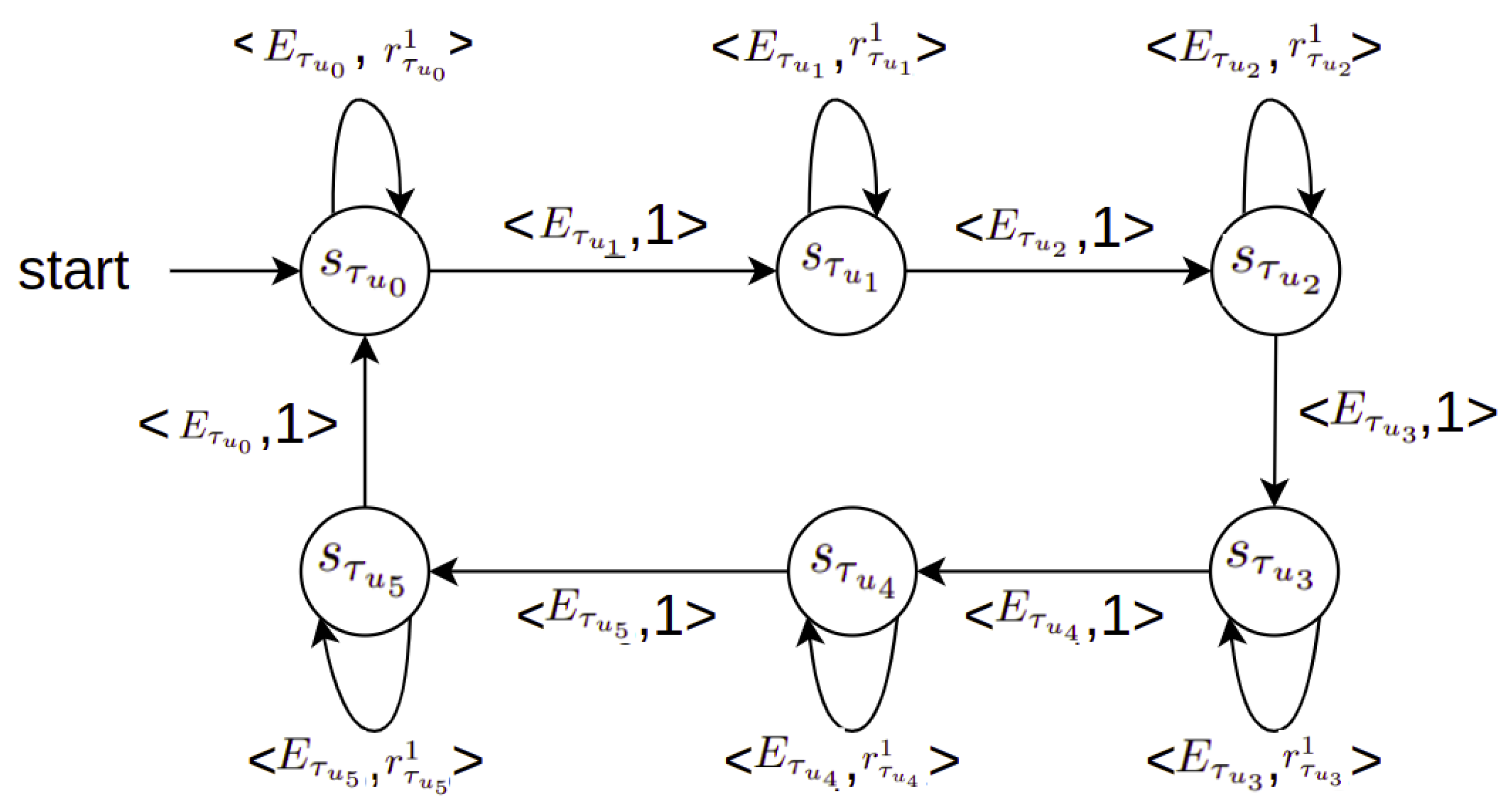
The learning method defines separate TRPO learners for different tasks and states, each with distinct ontology-based reward functions. These reward functions are designed to guide the learning process toward desirable scheduling outcomes, such as minimizing waiting time and maximizing machine utilization. Based on the ONTOADAPT-REWARD model, we propose the following method (see Figure 6):
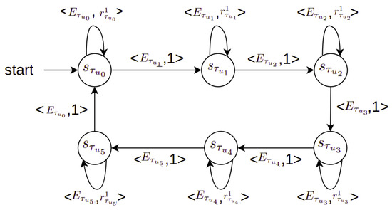
Figure 6.
A reward machine for the job shop scheduling environment. indicates the agent’s different states, are subsumers extracted from the agent’s states as new propositional symbols/events, and are the ontology-based reward functions. We assume that the agent receives a fixed reward value equal to 1 to transition from one state to the next.
In state , the agent defines three separate TRPO learners and for task with different reward functions respectively. For the sake of simplicity, for tasks and the agent uses a random strategy same as the baseline method; however, there is the possibility that the agent defines separate learners for task using ontology-based reward functions and for task with reward functions . The agent uses one learner for task with reward function (i.e., other learners can be defined using reward functions ). In state , in 4 out of 16 machines, the agent uses one learner for task with reward function (it is possible to launch two more learners for this task with reward functions and ). For the 12 machines left, the agent uses the baseline FIFO strategy. For task , the agent uses the random strategy same as the baseline method; however, the agent may define a separate learner for this task using the ontology-based reward function (see Table 3).
6.2. Model Evaluation
Ensuring the reliability of the RL-based model requires thorough evaluation of the training results. To evaluate the model, we implemented the following steps:
Performance Metrics Evaluation: To evaluate the proposed method’s performance, we use the following metrics:
- Average utilization rate of machines (see Equation (6)).
- Average waiting time : The average waiting time of orders is computed as follows:
- Total failed orders : The number of failed orders due to delay (i.e., due date requirement).
- Total processed orders : The count of successfully processed orders.
The performance of the baseline method is compared to that of our proposed method.
Scenario-based Validation: The model’s performance was validated across multiple scenarios with varying order loads and due date requirements (refer to Table 4). We conducted 10 runs for each scenario to ensure consistency and reliability of the results.

Table 4.
Job shop scheduling environment scenarios.
6.3. Results and Discussion
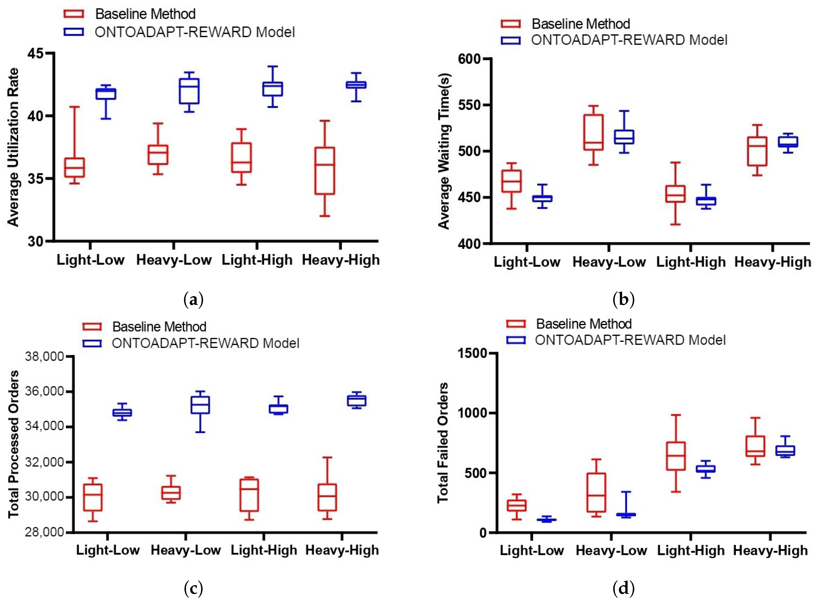
Figure 7 presents the average utilization rate, waiting time, total processed orders, and failed orders across 10 runs in each scenario for both the baseline method and the proposed ONTOADAPT-REWARD-based method. The results show that the proposed method increases the average utilization rate and the total processed orders and decreases the average waiting time and the total failed orders compared to the baseline method. We observe an increase in the total number of processed orders by 6%, 14%, 14%, and 15%, and the average utilization rate is increased by 5%, 11%, 12%, and 16% in Light-High, Light-Low, Heavy-High, and Heavy-Low scenarios, respectively (see Table 5). So, the percentage change is more significant when the number of orders increases. Also, the total failed orders are decreased by 68%, 73%, 41%, and 32%, and the average waiting time is decreased by 13%, 8%, 9%, and 6% in Light-High, Light-Low, Heavy-High, and Heavy-Low scenarios, respectively. The improvement in the Low scenarios is lower than in the High scenarios. This is because the number of low due date orders increases, and our proposed method shows less improvement due to the limited number of resources.
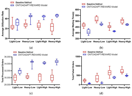
Figure 7.
The baseline method and the ONTOADAPT-REWARD-based proposed method (without multi-advisor RL). (a) Average utilization rate. (b) Average waiting time. (c) Total processed orders. (d) Total failed orders.

Table 5.
The percentage change in performance metrics: the baseline method and the ONTOADAPT-REWARD-based proposed method (without multi-advisor RL).
Similarly, compared to the baseline method, the ONTOADAPT-REWARD-based proposed method (with multi-advisor RL) increases the average utilization rate and the total number of processed orders while decreasing the average waiting time and the total number of failed orders (see Figure 8). We observe that the total processed orders is increased by 16%, 16%, 16%, and 18%, and the average utilization rate is increased by 15%, 14%, 16%, and 19% in Light-High, Light-Low, Heavy-High, and Heavy-Low scenarios, respectively (see Table 6). So, the percentage change is more significant with a high number of orders. Also, the total failed orders are decreased by 51%, 53%, 18%, and 4%, and the average waiting time is decreased by 3%, 0%, 1%, and −1% in Light-High, Light-Low, Heavy-High, and Heavy-Low scenarios, respectively. In Low scenarios, limited resources result in less improvement due to the increased number of low due date orders. When we compare the results of the proposed method with and without multi-advisor RL, we observe that the improvement without multi-advisor RL is more significant than the other one. The reason can be the multiple conflicting reward functions (objectives), which must be balanced based on their relative importance, so a simple voting algorithm does not work well, and a more comprehensive reward evaluation is required.
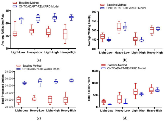
Figure 8.
The baseline method and the ONTOADAPT-REWARD-based proposed method (with multi-advisor RL). (a) Average utilization rate. (b) Average waiting time. (c) Total processed orders. (d) Total failed orders.

Table 6.
The percentage change in performance metrics: the baseline method and the ONTOADAPT-REWARD-based proposed method (with multi-advisor RL).
7. Conclusions and Future Work
Job Shop Scheduling (JSS) often involves conflicting objectives, dynamic factors, and intricate trade-offs between goals like minimizing production time and cost and maximizing resource utilization. Adaptive reward functions allow the Reinforcement Learning (RL) agent to dynamically prioritize these objectives based on evolving conditions, enabling more effective decision-making and resulting in more sustainable manufacturing by optimizing resource usage, machine usage, and reducing idle times.
The Reward Machine (RM) provides a structured, automata-based representation of a reward function for RL agents to decompose problems into subproblems that can be learned efficiently. RL agents can focus on learning and optimizing actions within these subproblems, leading to more efficient decision-making and improved scheduling outcomes. Additionally, RMs facilitate better generalization across different scheduling scenarios, enhancing the adaptability of RL-based job shop schedulers. As problems become more complex, the RM design can become cumbersome. In addition, RMs need to be adaptive when dealing with unexpected events in dynamic and partially observable environments. To create/modify RMs dynamically/adaptively through ontological knowledge, we propose an Ontology-based Adaptive Reward Machine (ONTOADAPT-REWARD) model.
In this paper, we have tested the proposed model in JSS scenarios, specifically applying it to a complex manufacturing environment involving various production stages. This research opens up multiple avenues for further exploration. In our future work, we will test ONTOADAPT-REWARD in additional scenarios. For instance, we could explore how the proposed solution performs when considering multiple production lines or non-deterministic production environments. While our current validation has been conducted in a simulated environment, we have a plan to test and refine our approach in real-world settings, considering more boundary conditions, starting from lead time to organizational and availability issues, tool wear, tool change, and maintenance. Future work could incorporate mechanisms to manage machine breakdowns by reallocating orders or rescheduling tasks to minimize downtime. Integrating predictive maintenance and machine health monitoring could help anticipate breakdowns and proactively adjust schedules. Agent-based modeling [65] can simulate the behavior of machines, maintenance processes, and scheduling decisions dynamically in response to changing conditions. For a comprehensive assessment of the energy-saving potential of the ONTOADAPT-REWARD model, future work could integrate energy-specific metrics into the evaluation framework. Moreover, our ONTOADAPT-REWARD model does not specifically address the material handling system (i.e., the movement, protection, storage, and control of materials) within the factory layout. Instead, it focuses on optimizing the scheduling and processing of orders through various machines and work areas. While the handling system undoubtedly impacts overall efficiency, our model assumes ideal conditions for material movement without explicitly modeling these dynamics. Future work could incorporate a more detailed handling system to explore its effects on scheduling decisions and overall manufacturing efficiency. Future research should also investigate the application of the ONTOADAPT-REWARD model to different production types, such as batch production, to generalize its applicability across various manufacturing processes and systems. This could involve adapting the model to handle the unique characteristics and constraints of batch production, including varying batch sizes, inter-batch setup times, and production sequencing.
The ontology used in the ONTOADAPT-REWARD model must be accurate and complete for the model to perform well. Dynamic environments require ontologies to evolve and update frequently, adapting to changing requirements. So, ontology evolution techniques [66] becomes crucial, for example, when production constraints may change over time. Comprehending, exploring, and exploiting an ontology-based schema can be complex, and summarization techniques [67,68] can be employed to provide a concise overview of critical concepts for better understanding and decision-making. In addition, concepts and properties within the ontology can differ depending on the specific context, such as during high-demand production periods, resource shortages, or power outages, leading to different ontologies for the RL agent to adapt accordingly. The impact of an incorrect belief about a property must be assessed to prevent scheduling errors. Additionally, a mechanism should be defined for dynamic weighting and objective priorities where there are multiple objectives in a manufacturing facility, including minimizing production costs, maximizing throughput, and minimizing job completion times simultaneously. Furthermore, actions with the same reward function should use a common learner to leverage the agent’s experiences efficiently and improve decision-making across various production stages. By using the relations defined in an ontology-based schema, it is possible to extract concepts related to each property, thereby reducing the agent’s state dimensionality for each learner and enhancing computational efficiency. It is especially important in a factory with hundreds of machines and jobs. Therefore, ONTOADAPT-REWARD is suitable for both small and large corporations due to its scalability. The model adapts to varying levels of complexity and size by concentrating on relevant concepts such as machine availability and order priorities, making it feasible to find optimal schedules efficiently regardless of the number of machines and jobs involved. Also, we can leverage the scalability of edge computing [69] to handle increasing data volumes and computational requirements as the manufacturing environment scales.
Author Contributions
Conceptualization, S.G.; methodology, S.G. and F.G.; validation, A.Z. and S.G.; writing—original draft preparation, S.G.; writing—review and editing, S.G., F.G. and A.Z.; visualization, A.Z. and S.G.; supervision, F.G.; F.G. and S.G. contributed equally to this paper. All authors have read and agreed to the published version of the manuscript.
Funding
This research was funded by Science Foundation Ireland grant number 21/RC/10295_P2.
Institutional Review Board Statement
Not applicable.
Informed Consent Statement
Not applicable.
Data Availability Statement
No new data were created or analyzed in this study. Data sharing is not applicable to this article.
Conflicts of Interest
The authors declare no conflicts of interest.
References
- Briefing, U.S. International energy outlook 2013. US Energy Inf. Adm. 2013, 506, 507. [Google Scholar]
- International Energy Agency. Global Energy Review 2022; International Energy Agency: Paris, France, 2022. [Google Scholar]
- Yin, L.; Li, X.; Gao, L.; Lu, C.; Zhang, Z. A novel mathematical model and multi-objective method for the low-carbon flexible job shop scheduling problem. Sustain. Comput. Inform. Syst. 2017, 13, 15–30. [Google Scholar] [CrossRef]
- Eslami, Y.; Lezoche, M.; Panetto, H.; Dassisti, M. On analysing sustainability assessment in manufacturing organisations: A survey. Int. J. Prod. Res. 2021, 59, 4108–4139. [Google Scholar] [CrossRef]
- Popper, J.; Motsch, W.; David, A.; Petzsche, T.; Ruskowski, M. Utilizing multi-agent deep reinforcement learning for flexible job shop scheduling under sustainable viewpoints. In Proceedings of the International Conference on Electrical, Computer, Communications and Mechatronics Engineering (ICECCME), Mauritius, 7–8 October 2021; IEEE: Piscataway, NJ, USA, 2021; pp. 1–6. [Google Scholar]
- Goutham, P.M.; Rohit, Y.; Nanjundeswaraswamy, T. A review on smart manufacturing, technologies and challenges. Int. Res. J. Eng. Technol. IRJET 2022, 9, 663–678. [Google Scholar]
- Yang, L.; Li, J.; Chao, F.; Hackney, P.; Flanagan, M. Job shop planning and scheduling for manufacturers with manual operations. Expert Syst. 2021, 38. [Google Scholar] [CrossRef]
- Pach, C.; Berger, T.; Sallez, Y.; Bonte, T.; Adam, E.; Trentesaux, D. Reactive and energy-aware scheduling of flexible manufacturing systems using potential fields. Comput. Ind. 2014, 65, 434–448. [Google Scholar] [CrossRef]
- Tang, D.; Dai, M. Energy-efficient approach to minimizing the energy consumption in an extended job-shop scheduling problem. Chin. J. Mech. Eng. 2015, 28, 1048–1055. [Google Scholar] [CrossRef]
- Yang, S.; Wang, D.; Chai, T.; Kendall, G. An improved constraint satisfaction adaptive neural network for job-shop scheduling. J. Sched. 2010, 13, 17–38. [Google Scholar] [CrossRef]
- Zhou, T.; Zhu, H.; Tang, D.; Liu, C.; Cai, Q.; Shi, W.; Gui, Y. Reinforcement learning for online optimization of job-shop scheduling in a smart manufacturing factory. Adv. Mech. Eng. 2022, 14, 1–19. [Google Scholar]
- Zeng, Y.; Liao, Z.; Dai, Y.; Wang, R.; Li, X.; Yuan, B. Hybrid intelligence for dynamic job-shop scheduling with deep reinforcement learning and attention mechanism. arXiv 2022, arXiv:2201.00548. [Google Scholar]
- Ghanadbashi, S.; Zarchini, A.; Golpayegani, F. An ontology-based augmented observation for decision-making in partially observable environments. In Proceedings of the International Conference on Agents and Artificial Intelligence (ICAART), Lisbon, Portugal, 22–24 February 2023; SCITEPRESS: Setubal, Portugal, 2023; pp. 343–354. [Google Scholar]
- Ghanadbashi, S. Ontology-enhanced decision-making for autonomous agents in dynamic and partially observable environments. arXiv 2024, arXiv:2405.17691. [Google Scholar]
- Wang, C.; Zeng, L. Optimization of multi-objective job-shop scheduling under uncertain environment. J. Eur. Syst. Autom. 2019, 52, 179–183. [Google Scholar] [CrossRef]
- Zhang, H.; Buchmeister, B.; Li, X.; Ojstersek, R. Advanced metaheuristic method for decision-making in a dynamic job shop scheduling environment. Mathematics 2021, 9, 909. [Google Scholar] [CrossRef]
- Cunha, B.; Madureira, A.M.; Fonseca, B.; Coelho, D. Deep reinforcement learning as a job shop scheduling solver: A literature review. In Proceedings of the Hybrid Intelligent Systems: 18th International Conference on Hybrid Intelligent Systems (HIS 2018), Porto, Portugal, 13–15 December 2018; Springer: Cham, Switzerland, 2020; pp. 350–359. [Google Scholar]
- Palacio, J.C.; Jiménez, Y.M.; Schietgat, L.; Van Doninck, B.; Nowé, A. A Q-Learning algorithm for flexible job shop scheduling in a real-world manufacturing scenario. Procedia CIRP 2022, 106, 227–232. [Google Scholar] [CrossRef]
- Cao, Z.; Zhou, L.; Hu, B.; Lin, C. An adaptive scheduling algorithm for dynamic jobs for dealing with the flexible job shop scheduling problem. Bus. Inf. Syst. Eng. 2019, 61, 299–309. [Google Scholar] [CrossRef]
- Bülbül, K.; Kaminsky, P. A linear programming-based method for job shop scheduling. J. Sched. 2013, 16, 161–183. [Google Scholar] [CrossRef]
- Yu, Y.; Ying, Y. The dynamic job shop scheduling approach based on data-driven genetic algorithm. Open Electr. Electron. Eng. J. 2014, 8, 41–45. [Google Scholar] [CrossRef]
- Bürgy, R. A neighborhood for complex job shop scheduling problems with regular objectives. J. Sched. 2017, 20, 391–422. [Google Scholar] [CrossRef]
- Nguyen, S.; Zhang, M.; Johnston, M.; Tan, K.C. Genetic programming for job shop scheduling. In Evolutionary and Swarm Intelligence Algorithms; Springer: Cham, Switzerland, 2019; pp. 143–167. [Google Scholar]
- Abdullah, S.; Abdolrazzagh-Nezhad, M. Fuzzy job-shop scheduling problems: A review. Inf. Sci. 2014, 278, 380–407. [Google Scholar] [CrossRef]
- Li, R.; Gong, W.; Lu, C. Self-adaptive multi-objective evolutionary algorithm for flexible job shop scheduling with fuzzy processing time. Comput. Ind. Eng. 2022, 168, 108099. [Google Scholar] [CrossRef]
- Pathak, D.; Agrawal, P.; Efros, A.A.; Darrell, T. Curiosity-driven exploration by self-supervised prediction. In Proceedings of the International Conference on Machine Learning (ICML), Sydney, NSW, Australia, 6–11 August 2017; PMLR: Breckenridge, CO, USA, 2017; pp. 2778–2787. [Google Scholar]
- Yang, D.; Tang, Y. Adaptive inner-reward shaping in sparse reward games. In Proceedings of the International Joint Conference on Neural Networks (IJCNN), Glasgow, UK, 19–24 July 2020; IEEE: New York, NY, USA, 2020; pp. 1–8. [Google Scholar]
- Hu, Y.; Wang, W.; Jia, H.; Wang, Y.; Chen, Y.; Hao, J.; Wu, F.; Fan, C. Learning to utilize shaping rewards: A new approach of reward shaping. Adv. Neural Inf. Process. Syst. 2020, 33, 15931–15941. [Google Scholar]
- De Hauwere, Y.M.; Devlin, S.; Kudenko, D.; Nowé, A. Context-sensitive reward shaping for sparse interaction multi-agent systems. Knowl. Eng. Rev. 2016, 31, 59–76. [Google Scholar] [CrossRef]
- Tenorio-Gonzalez, A.C.; Morales, E.F.; Villasenor-Pineda, L. Dynamic reward shaping: Training a robot by voice. In Proceedings of the Ibero-American Conference on Artificial Intelligence (IBERAMIA), Bahia Blanca, Argentina, 1–5 November 2010; Springer: Berlin/Heidelberg, Germany, 2010; pp. 483–492. [Google Scholar]
- Michini, B.; Cutler, M.; How, J.P. Scalable reward learning from demonstration. In Proceedings of the International Conference on Robotics and Automation (ICRA), Karlsruhe, Germany, 6–10 May 2013; IEEE: New York, NY, USA, 2013; pp. 303–308. [Google Scholar]
- Hadfield-Menell, D.; Milli, S.; Abbeel, P.; Russell, S.J.; Dragan, A. Inverse reward design. Adv. Neural Inf. Process. Syst. 2017, 30, 6765–6774. [Google Scholar]
- Baier, C.; Katoen, J.P. Principles of Model Checking; MIT Press: Cambridge, MA, USA, 2008. [Google Scholar]
- Wainwright, M.J.; Jordan, M.I. Graphical models, exponential families, and variational inference. Found. Trends Mach. Learn. 2008, 1, 1–305. [Google Scholar] [CrossRef]
- Toro Icarte, R.; Waldie, E.; Klassen, T.; Valenzano, R.; Castro, M.; McIlraith, S. Learning reward machines for partially observable reinforcement learning. Adv. Neural Inf. Process. Syst. 2019, 32, 15497–15508. [Google Scholar] [CrossRef]
- Furelos-Blanco, D.; Law, M.; Jonsson, A.; Broda, K.; Russo, A. Hierarchies of reward machines. arXiv 2022, arXiv:2205.15752. [Google Scholar]
- Zhou, W.; Li, W. A hierarchical bayesian approach to inverse reinforcement learning with symbolic reward machines. arXiv 2022, arXiv:2204.09772. [Google Scholar]
- Brewster, C.; O’Hara, K. Knowledge representation with ontologies: The present and future. IEEE Intell. Syst. 2004, 19, 72–81. [Google Scholar] [CrossRef]
- Ghanadbashi, S.; Zarchini, A.; Golpayegani, F. Ontology-based adaptive reward functions. In Proceedings of the Modelling and Representing Context (MRC) at 26th European Conference on Artificial Intelligence (ECAI), Krakow, Poland, 30 September–4 October; Springer: Berlin/Heidelberg, Germany, 2023; pp. 1–7. [Google Scholar]
- Chen, J.; Frank Chen, F. Adaptive scheduling and tool flow control in flexible job shops. Int. J. Prod. Res. IJPR 2008, 46, 4035–4059. [Google Scholar] [CrossRef]
- Zhang, B.X.; Yi, L.X.; Xiao, S. Study of stochastic job shop dynamic scheduling. In Proceedings of the International Conference on Machine Learning and Cybernetics, Guangzhou, China, 18–21 August 2005; IEEE: New York, NY, USA, 2005; Volume 2, pp. 911–916. [Google Scholar]
- Dominic, P.D.; Kaliyamoorthy, S.; Kumar, M.S. Efficient dispatching rules for dynamic job shop scheduling. Int. J. Adv. Manuf. Technol. 2004, 24, 70–75. [Google Scholar] [CrossRef]
- Chen, S.; Huang, Z.; Guo, H. An end-to-end deep learning method for dynamic job shop scheduling problem. Machines 2022, 10, 573. [Google Scholar] [CrossRef]
- Toro Icarte, R.; Klassen, T.; Valenzano, R.; McIlraith, S. Using reward machines for high-level task specification and decomposition in reinforcement learning. In Proceedings of the International Conference on Machine Learning (ICML), Stockholm, Sweden, 10–15 July 2018; PMLR: Breckenridge, CO, USA, 2018; pp. 2107–2116. [Google Scholar]
- Meuleau, N.; Peshkin, L.; Kim, K.E.; Kaelbling, L.P. Learning finite-state controllers for partially observable environments. arXiv 2013, arXiv:1301.6721. [Google Scholar]
- Mahmud, M.M.H. Constructing states for reinforcement learning. In Proceedings of the International Conference on Machine Learning (ICML), Haifa, Israel, 21–24 June 2010; OmniPress: West Norriton, PA, USA, 2010; pp. 727–734. [Google Scholar]
- Ghanadbashi, S.; Golpayegani, F. Using ontology to guide reinforcement learning agents in unseen situations. Appl. Intell. APIN 2022, 52, 1808–1824. [Google Scholar] [CrossRef]
- Ng, A.Y.; Harada, D.; Russell, S. Policy invariance under reward transformations: Theory and application to reward shaping. In Proceedings of the International Conference on Machine Learning (ICML), Bled, Slovenia, 27–30 June 1999; Volume 99, pp. 278–287. [Google Scholar]
- Mannion, P.; Devlin, S.; Duggan, J.; Howley, E. Reward shaping for knowledge-based multi-objective multi-agent reinforcement learning. Knowl. Eng. Rev. 2018, 33, e23. [Google Scholar] [CrossRef]
- Laud, A.D. Theory and Application of Reward Shaping in Reinforcement Learning. Ph.D. Thesis, University of Illinois at Urbana-Champaign, Urbana, IL, USA, 2004. [Google Scholar]
- Zou, H.; Ren, T.; Yan, D.; Su, H.; Zhu, J. Reward shaping via meta-learning. arXiv 2019, arXiv:1901.09330. [Google Scholar]
- Niekum, S.; Spector, L.; Barto, A. Evolution of reward functions for reinforcement learning. In Proceedings of the Genetic and Evolutionary Computation Conference (GECCO), Dublin, Ireland, 12–16 July 2011; pp. 177–178. [Google Scholar]
- Hussein, A.; Elyan, E.; Gaber, M.M.; Jayne, C. Deep reward shaping from demonstrations. In Proceedings of the International Joint Conference on Neural Networks (IJCNN), Anchorage, AK, USA, 14–19 May 2017; IEEE: New Yoek, NY, USA, 2017; pp. 510–517. [Google Scholar]
- Schulman, J.; Levine, S.; Abbeel, P.; Jordan, M.; Moritz, P. Trust region policy optimization. In Proceedings of the International Conference on Machine Learning (ICML), Lille, France, 7–9 July 2015; PMLR: Breckenridge, CO, USA, 2015; pp. 1889–1897. [Google Scholar]
- Sutton, R.S.; Barto, A.G. Reinforcement Learning: An Introduction; MIT Press: Cambridge, MA, USA, 2018. [Google Scholar]
- Zouaq, A.; Nkambou, R. A survey of domain ontology engineering: Methods and tools. In Advances in Intelligent Tutoring Systems; Springer: Berlin/Heidelberg, Germany, 2010; pp. 103–119. [Google Scholar]
- Alsubait, T.; Parsia, B.; Sattler, U. Measuring similarity in ontologies: A new family of measures. In Proceedings of the International Conference on Knowledge Engineering and Knowledge Management (EKAW), Linkoping, Sweden, 24–28 November 2014; Springer: Berlin/Heidelberg, Germany, 2014; pp. 13–25. [Google Scholar]
- Pfitzer, F.; Provost, J.; Mieth, C.; Liertz, W. Event-driven production rescheduling in job shop environments. In Proceedings of the International Conference on Automation Science and Engineering (CASE), Munich, Germany, 20–24 August 2018; IEEE: New Yoek, NY, USA, 2018; pp. 939–944. [Google Scholar]
- Buchmeister, B.; Ojstersek, R.; Palcic, I. Advanced methods for job shop scheduling. Adv. Prod. Ind. Eng. APEM 2017, 31. [Google Scholar] [CrossRef]
- Kuhnle, A. Simulation and Reinforcement Learning Framework for Production Planning and Control of Complex Job Shop Manufacturing Systems. 2020. Available online: https://github.com/AndreasKuhnle/SimRLFab (accessed on 1 June 2022).
- Haller, A.; Janowicz, K.; Cox, S.J.; Lefrançois, M.; Taylor, K.; Le Phuoc, D.; Lieberman, J.; García-Castro, R.; Atkinson, R.; Stadler, C. The modular SSN ontology: A joint W3C and OGC standard specifying the semantics of sensors, observations, sampling, and actuation. Semant. Web 2019, 10, 9–32. [Google Scholar] [CrossRef]
- Duy, T.K.; Quirchmayr, G.; Tjoa, A.; Hanh, H.H. A semantic data model for the interpretion of environmental streaming data. In Proceedings of the International Conference on Information Science and Technology (ICIST), Nis, Serbia, 28–30 June 2017; IEEE: New York, NY, USA, 2017; pp. 376–380. [Google Scholar]
- Laroche, R.; Fatemi, M.; Romoff, J.; van Seijen, H. Multi-advisor reinforcement learning. arXiv 2017, arXiv:1704.00756. [Google Scholar]
- Kuhnle, A.; Röhrig, N.; Lanza, G. Autonomous order dispatching in the semiconductor industry using reinforcement learning. Procedia CIRP 2019, 79, 391–396. [Google Scholar] [CrossRef]
- Golpayegani, F.; Clarke, S. Co-Ride: Collaborative preference-based taxi-sharing and taxi-dispatch. In Proceedings of the IEEE 30th International Conference on Tools with Artificial Intelligence, ICTAI 2018, Volos, Greece, 5–7 November 2018; Tsoukalas, L.H., Grégoire, É., Alamaniotis, M., Eds.; IEEE: New York, NY, USA, 2018; pp. 864–871. [Google Scholar] [CrossRef]
- Zablith, F.; Antoniou, G.; d’Aquin, M.; Flouris, G.; Kondylakis, H.; Motta, E.; Plexousakis, D.; Sabou, M. Ontology evolution: A process-centric survey. Knowl. Eng. Rev. KER 2015, 30, 45–75. [Google Scholar] [CrossRef]
- Pires, C.E.; Sousa, P.; Kedad, Z.; Salgado, A.C. Summarizing ontology-based schemas in PDMS. In Proceedings of the International Conference on Data Engineering Workshops (ICDEW), Long Beach, CA, USA, 1–6 March 2010; IEEE: New York, NY, USA, 2010; pp. 239–244. [Google Scholar]
- Pouriyeh, S.; Allahyari, M.; Kochut, K.; Arabnia, H.R. A comprehensive survey of ontology summarization: Measures and methods. arXiv 2018, arXiv:1801.01937. [Google Scholar]
- Golpayegani, F.; Chen, N.; Afraz, N.; Gyamfi, E.; Malekjafarian, A.; Schäfer, D.; Krupitzer, C. Adaptation in Edge Computing: A Review on Design Principles and Research Challenges; ACM Transactions on Autonomous and Adaptive Systems: New York, NY, USA, 2024. [Google Scholar]
Disclaimer/Publisher’s Note: The statements, opinions and data contained in all publications are solely those of the individual author(s) and contributor(s) and not of MDPI and/or the editor(s). MDPI and/or the editor(s) disclaim responsibility for any injury to people or property resulting from any ideas, methods, instructions or products referred to in the content. |
© 2024 by the authors. Licensee MDPI, Basel, Switzerland. This article is an open access article distributed under the terms and conditions of the Creative Commons Attribution (CC BY) license (https://creativecommons.org/licenses/by/4.0/).

