Short-Term Photovoltaic Power Generation Prediction Based on Copula Function and CNN-CosAttention-Transformer

Abstract

The intermittent nature of solar energy poses significant challenges to the integration of photovoltaic (PV) power generation into the electrical grid. Consequently, the precise forecasting of PV power output becomes essential for efficient real-time power system dispatch. To meet this demand, this paper proposes a deep learning model, the CA-Transformer, specifically designed for PV power output prediction. To overcome the shortcomings of traditional correlation coefficient methods in dealing with nonlinear relationships, this study utilizes the Copula function. This approach allows for a more flexible and accurate determination of correlations within time series data, enabling the selection of features that exhibit a high degree of correlation with PV power output. Given the unique data characteristics of PV power output, the proposed model employs a 1D-CNN model to identify local patterns and trends within the time series data. Simultaneously, it implements a cosine similarity attention mechanism to detect long-range dependencies within the time series. It then leverages a parallel structure of a 1D-CNN and a cosine similarity attention mechanism to capture patterns across varying time scales and integrate them. In order to show the effectiveness of the model proposed in this study, its prediction results were compared with those of other models (LSTM and Transformer). The experimental results demonstrate that our model outperforms in terms of PV power output prediction, thereby offering a robust tool for the intelligent management of PV power generation.

1. Introduction

With the acceleration of globalization and the intensification of industrialization, the global energy demand continues to escalate. However, the extensive extraction and use of traditional fossil fuels have not only intensified the strain on energy supplies but have also led to serious environmental issues. The emission of greenhouse gases during the combustion of fossil fuels is a principal driver of global warming, which disrupts the Earth’s climate system, adversely affects biodiversity, and deteriorates human living conditions. Against this backdrop, the development and utilization of renewable energy sources become particularly significant. Photovoltaic (PV) power generation, as a clean and renewable form of energy, holds tremendous potential and is considered an effective approach to addressing the energy crisis and alleviating environmental stress. PV technology, through the direct conversion of solar irradiance into electrical energy, can diminish the dependence on fossil fuels and curtail greenhouse gas emissions, thereby mitigating global warming [1,2,3]. However, the efficiency and output of PV power generation are influenced by various meteorological conditions, such as sunlight intensity, temperature, and cloud cover, leading to uncertainty and volatility in PV power generation. This instability poses challenges to the stable operation of the power grid, especially when PV power is integrated on a large scale [4]. To address this issue, researchers and engineers are exploring the use of deep learning and other advanced data analysis techniques to predict PV power generation. By analyzing historical weather data and power generation records from PV stations, accurate prediction models can be established to forecast power generation over future periods. Such predictive models not only aid grid operators in optimizing resource allocation and maintaining grid stability but also facilitate the large-scale deployment of PV power generation and expedite the adoption of renewable energy. Moreover, accurate PV power generation predictions are strategically significant for achieving China’s “dual carbon” goals—carbon peaking and carbon neutrality. With continuous advancements in PV technology and cost reductions, it is expected that PV power generation will occupy an increasingly Important position in the future energy structure, contributing significantly to the realization of a low-carbon economy and sustainable development [5]. Therefore, the development of efficient PV power generation prediction technology not only helps improve the operational efficiency of power systems but also supports the global long-term effort to combat climate change. The research and applications in this field will undoubtedly have a profound impact on future energy and environmental policies.

According to the prediction time scale, photovoltaic forecasting can be divided into ultra-short term, short term, medium term, and long term [6]. Among them, medium- and long-term forecasts often exhibit significant errors due to weather fluctuations and error accumulation. On the other hand, short-term and ultra-short-term forecasts demonstrate higher accuracy, providing assurance for the real-time scheduling of the power system [7]. Currently, the methods for photovoltaic power forecasting can be primarily categorized into three types: physical models, statistical models, and artificial intelligence models [8,9,10,11,12].

Physical methods are a type of predictive approach based on theoretical simulation models. They do not rely on historical data but instead combine numerical weather prediction (NWP) [13] with the installation characteristics of photovoltaic devices, such as the solar panel tilt angle and conversion efficiency, to forecast photovoltaic power generation. NWP is a mathematical model based on fluid mechanics and thermodynamics, incorporating observational data from satellites, radars, and weather stations to simulate the evolution of the atmosphere. However, due to the heavy reliance on NWP, physical methods suffer from longer intervals in generating meteorological data and require substantial time and computational resources, thereby limiting their application in short-term photovoltaic power prediction [14].

Statistical methods, such as fuzzy theory [15], gray theory [16], Markov chains (MCs) [17], linear regression [18], and autoregressive (AR) [19] models, are commonly used to reveal mathematical relationships within data, often assuming linearity. These traditional techniques are widely employed in analyzing historical data to establish prediction models. However, they have limitations when dealing with nonlinear relationships and complex time-series data. Their effectiveness in extracting deep-level features is inadequate, and the dynamic and non-periodic characteristics of photovoltaic data make it more challenging to establish accurate prediction models using statistical methods. The unstable relationship between inputs and outputs may lead to less accurate performance when making predictions under extreme weather conditions [20].

Artificial intelligence (AI) models can learn from large-scale data, discover complex patterns and regularities, extract features from training data, and generalize to unseen data, thereby enhancing their predictive and reasoning abilities [21]. These AI models encompass various techniques, including decision trees [22], support vector machines (SVMs) [23], naive Bayes, random forests [24,25], and neural networks. In the early days of AI modeling, Antonanzas et al. [26] applied SVM and random forest (RF) machine learning techniques to short-term photovoltaic (PV) power forecasting based on numerical weather prediction (NWP). However, these models exhibited subpar performance when dealing with large datasets, primarily due to their high data quality requirements [27]. Consequently, an increasing number of researchers have shifted their focus toward deep learning models. Deep learning, known for its ability to generalize and automatically extract abstract representations, surpasses traditional machine learning [28] approaches. It can extract features from intricate data and map them to meaningful outcomes. Currently, in neural networks for short-term PV power forecasting, commonly used architectures include recurrent neural networks (RNNs), long short-term memory (LSTM) networks, convolutional neural networks (CNNs), and the Transformer. Gao et al. proposed a time-series forecasting method based on ideal and non-ideal weather conditions. For ideal weather scenarios, they introduced an LSTM network that leveraged next-day meteorological data. To address non-ideal weather situations, they incorporated neighboring daily time series and typical weather-type information for prediction [29]. Agga et al. introduced two hybrid models (CNN-LSTM and ConvLSTM) for the efficient prediction of self-consumption PV station generation. Experimental results demonstrated that their approach outperformed regular LSTM models in terms of accuracy [30]. Dai et al. enhanced the gated recurrent unit (GRU) by adding a RepeatVector layer and a TimeDistributed layer, resulting in a more diverse GRU architecture. To mitigate the impact of data fluctuations on prediction accuracy, they compared various data smoothing techniques, showing that their method was better suited for short-term forecasting [31]. Zhen et al. proposed an improved genetic algorithm-based bidirectional LSTM (GA-BiLSTM) model for ultra-short-term PV power prediction. Even without meteorological data, they innovatively fused output sequences from neighboring PV stations as inputs to the prediction model. The results indicated that their model achieved the lowest RMSE values for 5-min, 15-min, and 30-min-ahead production forecasts, i.e., 0.438, 0.806, and 1.118, respectively, demonstrating superior performance in ultra-short-term predictions [32].

The encoder–decoder architecture is a commonly used deep learning model framework, which is a general term for a class of algorithms and does not specifically refer to a particular algorithm. Under this framework, different algorithms can be used to solve different tasks. The sequence-to-sequence model of the encoder–decoder structure can meet the demand for higher-accuracy photovoltaic power generation prediction. As a popular deep learning model, the Transformer was initially applied in Natural Language Processing (NLP) and performed excellently [33] and was later applied to photovoltaic power generation prediction. Compared with the traditional recurrent neural network (RNN) and convolutional neural network (CNN), the self-attention mechanism used by the Transformer can directly model the dependency relationship between any two positions in the sequence, effectively capture long-distance context information, and better handle long-term dependencies. Zhao Z and others used the Transformer network for photovoltaic power generation prediction, and the proposed model used the LightGBM and k-means algorithms to create a similar day selection approach [34].

The current photovoltaic power generation prediction methods have solved many problems in this field, but there are still some shortcomings. For example, to make accurate predictions and reduce training time, it is necessary to extract the key meteorological factors that affect photovoltaic power generation. The commonly used algorithms cannot fully measure the nonlinearity and trend correlations between photovoltaic power generation and meteorological factors. There are many meteorological factors that affect photovoltaic power generation, and they are complex and changeable, and their effects are different. Effectively extracting the main meteorological factors is the key to improving prediction accuracy. The most commonly used algorithms include correlation analysis, gray correlation, and principal component analysis. Traditional correlation analysis mainly uses linear correlation coefficients to measure the correlation between variables, and it can only measure the strength of linear relationships and is insensitive to nonlinear relationships. The optimal values of some indicators of the gray correlation analysis method are difficult to determine, and there may be problems of excessive subjectivity. The principal component analysis method assumes that the data are linearly separable, and the effect may not be good for data with nonlinear relationships; it also only considers the variance in the data, ignoring other statistical characteristics and potentially losing some important information. These analyses can quantify the correlation between meteorological factors and photovoltaic power generation to a certain extent. However, in actual situations, these methods do not work well because most meteorological factors and photovoltaic power generation have nonlinear relationships. The Copula method overcomes the assumption of a linear correlation in traditional normal distribution models. It not only takes into account the marginal distributions but also considers the correlation structure between variables. This allows for a more flexible and robust measurement of nonlinear and asymmetric relationships between time series, making it suitable for selecting meteorological factors highly correlated with photovoltaic power generation. At the same time, the Copula function has some limitations; for example, the estimation of the parameters of the Copula function may not reach the optimum.

The main structure of this paper is as follows: Section 1 introduces the current state of research and the contributions of this paper; Section 2 introduces the various parts of the model, including the basic theory of the Copula function, CNN, Transformer, and cosine self-attention; Section 3 introduces the method of calculating correlations with the Copula function, the proposed hybrid model framework (CA-Transformer), and evaluation metrics; Section 4 presents case studies and the discussion; and Section 5 concludes the paper.

Therefore, based on the characteristics of time-series data, this paper proposes a CNN-CosAttention-Transformer (CA-Transformer) model based on the Copula function. The contributions of this paper are as follows:

(1)

To solve the problem of the poor performance of some traditional correlation coefficient methods, the Copula function is used to calculate the correlation coefficient, which can more flexibly and accurately measure the nonlinear and asymmetrical correlation relationships between time series, and is used to select features with high correlations with photovoltaic power generation power.

(2)

Considering the data characteristics of photovoltaic power generation power, the 1D-CNN model is used to capture local patterns and trends in time-series data, while the attention mechanism based on cosine similarity is used to capture long-distance dependencies in time-series data, and its attention focus is dynamically adjusted according to the current input.

(3)

The CA-Transformer model is established, using the parallel structure of the CNN and CosAttention to capture patterns at different time scales, and is compared with other models (LSTM, Transformer), proving the effectiveness of the model.

2. Background Theories

2.1. Basic Theory of Copula Functions

The primary function of the Copula is to describe and model the dependency structure between two or more random variables. The Sklar theorem, which reflects how the Copula “connects” marginal distributions, holds an important position in Copula theory.

Taking a binary example, let $H\left(x_1, x_2\right)$ be the joint distribution function of random variables $x_1$ and $x_2$, and let $F_1\left(x_1\right)$ and $F_2\left(x_2\right)$ be their respective marginal distribution functions. Then, there exists a Copula function C such that $H\left(x_1, x_2\right) = C\left(F_1\left(x_1\right), F_2\left(x_2\right)\right)$ holds for all x₁ and x₂. If $F_1\left(x_1\right)$ and $F_2\left(x_2\right)$ are continuous, then C is unique. Conversely, if C is a Copula function and $F_1\left(x_1\right)$ and $F_2\left(x_2\right)$ are the marginal distribution functions of $x_1$ and $x_2$, then $H\left(x_1, x_2\right)$, defined by $H\left(x_1, x_2\right) = C\left(F_1\left(x_1\right), F_2\left(x_2\right)\right)$, is the joint distribution function of random variables $x_1$ and $x_2$.

From the above theorem, the following corollary can be derived. Let $H\left(x_1, x_2\right)$ be the joint distribution function of random variables $x_1$ and $x_2$, let $F_1\left(x_1\right)$ and $F_2\left(x_2\right)$ be their respective marginal distribution functions, and let $F_1^{-1}\left(u_1\right)$ and $F_2^{-1}\left(u_2\right)$ represent the inverse functions of $F_1\left(x_1\right)$ and $F_2\left(x_2\right)$, with $u_1=F_1\left(x_1\right)$ and $u_2=F_2\left(x_2\right)$. Then, the Copula function can be expressed as follows:

$$C\left(u_1,u_2\right)=H\left(F_1^{-1}\left(u_1\right),F_2^{-1}\left(u_2\right)\right)$$

(1)

There are many common Copula functions. This paper introduces five types used: Normal Copula, t-Copula, Gumbel Copula, Clayton Copula, and Frank Copula. Their formulas and parameters are shown in

Table 1. Formulas for five Copula functions and explanation of parameters.

Copula	Functional Form	Parameters
Normal	$\mathsf{\Phi }\left({\mathsf{\Phi }}^{-1}\left(u_1\right),\dots ,{\mathsf{\Phi }}^{-1}\left(u_d\right)\right)$	$\mathsf{\Sigma }=\left[\begin{array}{ccc}1& \dots & {\rho }_{1d}\\ ⋮& \ddots & ⋮\\ {\rho }_{1d}& \dots & 1\end{array}\right]$
T	$T_{\mathsf{\Sigma },v}\left(T_v^{-1}\left(u_1\right),\dots ,T_v^{-1}\left(u_d\right)\right)$	$\mathsf{\Sigma }=\left[\begin{array}{ccc}1& \dots & {\rho }_{1d}\\ ⋮& \ddots & ⋮\\ {\rho }_{1d}& \dots & 1\end{array}\right]$
Frank	$-\frac{1}{\theta }ln\left[1+\frac{{\mathsf{\Pi }}_{j=1}^d\left(e^{-\theta u_j}-1\right)}{{(e^{-\theta }-1)}^{d-1}}\right]$	$\theta \in ℝ\setminus 0$
Clayton	${\left[\left({\mathsf{\Sigma }}_{\mathrm{j}=1}^d{u}_{\mathrm{j}}^{-\theta }\right)-d+1\right]}^{-\frac{1}{\theta }}$	$\theta \in \left[-1,\infty \right]\setminus 0$
Gumbel	$\exp {\left\{-\left[{\mathsf{\Sigma }}_{\mathrm{j}=1}^d{(-ln{u}_{\mathrm{j}})}^{\theta }\right]\right\}}^{\frac{1}{\theta }}$	$\theta \in \left[1,\infty \right]$

.

2.2. Convolutional Neural Network

Convolutional neural networks (CNNs) are a type of deep learning algorithm characterized by their ability to automatically and adaptively learn the spatial hierarchical structure of local data. In the model proposed in this paper, a CNN is used to capture the local patterns and spatial features of the input data. A CNN consists of multiple layers, including the input layer, convolutional layer, pooling layer, fully connected layer, and output layer. Each layer performs specific operations to extract useful information from the input data, as shown in the classic CNN structure in Figure 1.

The convolutional layer is a fundamental component of a convolutional neural network (CNN). It employs a set of learnable filters (also known as convolutional kernels) to perform convolutional operations on input data. Each filter can detect specific features within the input data. The calculation process for convolution is illustrated in Figure 1. In this example, we have a 2 × 2 convolutional kernel. With a stride of 1, the kernel slides one unit to the right until it reaches the rightmost edge of the input matrix. Then, it moves one unit down and returns to the leftmost side, repeating the rightward movement. At each step, the kernel multiplies the corresponding numbers in the input matrix and adds them up. Pooling layers are used to reduce data dimensions and computational complexity. Figure 1 also demonstrates max pooling, where a 2 × 2 region selects the maximum value for output.

A CNN possesses three main characteristics: local connectivity, weight sharing, and translation invariance. Local connectivity is reflected in the fact that, in a CNN, neurons are only connected to a local region of the previous layer rather than to all neurons in the previous layer. This local connection method effectively reduces the number of parameters and improves computational efficiency. The characteristic of weight sharing allows a CNN to use the same convolutional kernel at different positions in the data with the same parameters. This parameter-sharing method significantly reduces the number of model parameters and enhances the model’s generalization ability. Translation invariance is due to the sliding of the convolution operation over the entire input data. Therefore, the same feature can be detected regardless of where it appears in the data.

In the domain of time-series forecasting, one-dimensional convolutional neural networks (1D-CNNs) are employed to process sequential data. Distinct from the two-dimensional convolutions tailored for imagery, 1D-CNNs perform convolutions along a singular spatial dimension, rendering them exceptionally adept at discerning temporal patterns and tendencies. PV power generation data are time-series data, where each data point is related to the data points before and after it, and the closer the data points are to the current prediction, the more information is available about them. A 1D-CNN can capture local temporal dependencies by adjusting the size of the convolutional kernel so that a smaller convolution kernel applies convolutional operations over a sliding window of the input data. And, they are able to capture local dependencies in time series with a smaller number of parameters due to the weight sharing and local connectivity properties.

2.3. CosAttention

The self-attention mechanism is a technique capable of capturing long-distance dependencies in input sequences. It determines the importance of each element by calculating the similarity between input elements. When processing sequence data, it allows each element to establish associations with other elements in the sequence, rather than just depending on adjacent elements. This mechanism can help the model better understand the context information in the sequence, thereby processing sequence data more accurately. In the model proposed in this paper, cosine self-attention is used to capture the global dependencies in the original data.

As the name suggests, the cosine similarity method uses the cosine value of the angle between two vectors to measure the importance between vectors. The larger the cosine value, the stronger the association between the two vectors. The formula for cosine similarity is as follows:

$$\mathrm{Attention}\left(Q,K,V\right)=\mathrm{softmax}\left(\frac{Q{K}^T}{\parallel Q\parallel \parallel K\parallel }\right)V$$

(2)

where Q, K, and V represent query, key, and value, respectively. $\parallel Q\parallel$ and $\parallel K\parallel$ represent the norms of Q and K, which are calculated by squaring all elements, summing them up, and then taking the square root.

2.4. Transformer

The Transformer model [31], proposed by Google’s research team in 2017, was designed to address the shortcomings of traditional sequence-to-sequence models in handling long-distance dependencies. The core of this model is the self-attention mechanism, which allows the model to dynamically focus on different positions of information when processing sequence data, thereby better capturing semantic relationships within the sequence. Over the past few years, research on the Transformer has applied it to various fields, including time-series prediction.

Since the Transformer itself does not have the ability to handle sequential information in the sequence, the model uses a position-encoding method to encode the position information of the elements in the sequence. The position-encoding layer uses a combination of sine and cosine functions to generate a unique encoding for each position in the sequence. The calculation formula for positional encoding is as follows:

$$\begin{array}{c}P{E}_{\left(pos,2i\right)}=sin\left(pos/{10000}^{2i/d_{model}}\right)\\ P{E}_{\left(pos,2i+1\right)}=cos\left(pos/{10000}^{2i/d_{model}}\right)\end{array}$$

(3)

Here, pos is the position of the element in the sequence, I is the index of the dimension, and $d_{model}$ is the dimension of the embedding vector in the model.

In the Transformer, the self-attention mechanism is a core component. It calculates the relevance scores between different positions in the sequence and transforms these scores into attention weights, thereby achieving a global understanding of the sequence. This mechanism allows the model to establish global semantic associations between different positions and adaptively learn the dependencies between different positions. The Transformer uses a scaled dot-product attention mechanism. The scaled dot-product attention mechanism is a method for calculating attention weights and is widely used in the self-attention mechanism. In the scaled dot-product attention mechanism, the query vector Q and the key vector K perform dot-product operations, and then the result is divided by a scaling factor, namely, $\sqrt{d_k}$, where $d_k$ is the dimension of the vector. The role of this scaling factor is to prevent the dot-product results from being too large or too small, thereby making the input of the softmax function more stable. Finally, the obtained scores are normalized through the softmax function to obtain attention weights. The advantage of the scaled dot-product attention mechanism is that it is fast in computation and can be implemented using highly optimized matrix multiplication code. The formula for scaled dot-product attention is as follows:

$$\mathrm{Attention}\left(Q,K,V\right)=\mathrm{softmax}\left(\frac{Q{K}^T}{\sqrt{d_k}}\right)\mathrm{V}$$

(4)

The multi-head attention mechanism used by the Transformer further enhances the model’s capabilities. By projecting the input into multiple different subspaces separately, calculating the attention weights of each subspace, and finally, combining these representations, it captures richer semantic information. This mechanism not only improves the model’s expressive power but also helps reduce overfitting and improve the generalization ability. The formula for multi-head attention is as follows:

$$\begin{array}{c}\mathrm{MultiHead}\left(Q,K,V\right)=\mathrm{Concat}\left({\mathrm{head}}_1,\dots ,{\mathrm{head}}_{\mathrm{h}}\right)W^O\\ \mathrm{where} {\mathrm{head}}_{\mathrm{i}}=\mathrm{Attention}\left(Q{W}_i^Q,K{W}_i^K,V{W}_i^V\right)\end{array}$$

(5)

where, $W_i^Q,W_i^K,W_i^V,W^O$ are all learnable parameters, and the dimension of the matrix is $W_i^Q\in {\mathrm{R}}^{d_{\mathrm{model}}\times d_k},W_i^K\in {\mathrm{R}}^{d_{\mathrm{model}}\times d_k},W_i^V\in {\mathrm{R}}^{d_{\mathrm{model}}\times d_v},W^O\in {\mathrm{R}}^{h{d}_v\times d_{\mathrm{model}}}$.

The Transformer model adopts an encoder–decoder architecture, where the encoder consists of multiple encoding layers, each of which uses a self-attention mechanism to process input data and determine which parts of the data are related to each other. The decoder reads the output of the encoder and uses the integrated context information to generate the output sequence.

Due to its parallel computing characteristics, the Transformer model has a significant advantage in training efficiency and can handle larger-scale datasets. These characteristics have gradually led to the application of the Transformer model in various fields.

3. Model Construction and Evaluation Metrics

3.1. Copula Function Correlation Analysis Method

The process of conducting correlation analysis using Copula functions primarily involves the following steps:

Data Acquisition and Preprocessing: Obtain historical power and meteorological data from photovoltaic power stations in a specific region and preprocess the data. Identify and handle anomalies and missing data by supplementing them with data from preceding and following moments or mid-scale data.

Estimation of Marginal Distribution Function: Use non-parametric kernel density estimation to estimate the marginal distribution function of random variables. Suppose $x_1,x_2,\cdots ,x_n$ are n sample points independently and identically distributed as F, with the probability density function denoted by $\left(x\right)$. The kernel density estimation function $\widehat{f_h}\left(x\right)$ is defined as follows:

$$\widehat{f_h}\left(x\right)=\frac{1}{nh}{\displaystyle \sum }_{i=1}^{n}K\left(\frac{x-x_i}{h}\right)$$

(6)

where x is the point whose probability density is to be estimated, $x_i$ is the sample point, $h>0$ is the bandwidth determining the width of the kernel function, and $K$ is the kernel function.

Parameter Estimation of Binary Copula Models: Use the maximum-likelihood estimation method and the marginal distribution function obtained in step two to solve for the parameter values of each binary Copula model.

Let $\left(x_{1i},x_{2i}\right)$ be drawn from the population $\left(X_1,X_2\right)$, where $i=1,2,\dots ,n$. $n$ represents the sample size, and $x_{1i},x_{2i}$ denote a meteorological factor and photovoltaic power, respectively. The marginal distribution functions of $x_{1i},x_{2i}$ are denoted by $F_1\left(x_{1i};{\theta }_1\right)$ and $F_2\left(x_{2i};{\theta }_2\right)$, with the corresponding probability density functions $f_1\left(x_{1i};{\theta }_1\right)$ and $f_2\left(x_{2i};{\theta }_2\right)$. ${\theta }_1$ and ${\theta }_2$ represent parameter vectors for the meteorological factor and photovoltaic power, respectively. The selected bivariate Copula joint distribution model is denoted by $C\left(F_1,F_2;\alpha \right)$, where $\alpha$ is the parameter vector for the bivariate Copula model. The logarithm of the likelihood function is given by

$$\ln L\left({\theta }_1,{\theta }_2,\alpha \right)={\displaystyle \sum }_{i=1}^n\ln C\left[F_1\left(x_{1i};{\theta }_1\right),F_2\left(x_{2i};{\theta }_2\right),\alpha \right]+{\displaystyle \sum }_{i=1}^n\ln f_1\left(x_{1i};{\theta }_1\right)+{\displaystyle \sum }_{i=1}^n\ln f_2\left(x_{2i};{\theta }_2\right)$$

(7)

By maximizing the logarithm of the likelihood function, we can obtain the estimated values of the Copula function parameters:

$$\left({\widehat{\theta }}_1,{\widehat{\theta }}_2,\widehat{\alpha }\right)=\mathrm{argmax}lnL\left({\theta }_1,{\theta }_2,\alpha \right)$$

(8)

Evaluation of Binary Copula Joint Distribution Models for Each Meteorological Factor: For each meteorological factor, we evaluate the corresponding binary Copula joint distribution models. We establish empirical Copula models using empirical Copula functions and calculate the squared Euclidean distance between each binary Copula model and the empirical Copula model for the same meteorological factor. This allows us to assess the relative performance of various binary Copula models.

Let $\left(x_{1i},x_{2i}\right)$, $i=1,2,\dots ,n$ be drawn from the population $\left(X_1,X_2\right)$. The empirical distribution functions of $X_1$ and $X_2$ are $F_1\left(x_{1i}\right)$ and $F_2\left(x_{2i}\right)$, respectively. The empirical Copula function of the sample is defined as follows:

$$\widehat{C_n}\left(u_1,u_2\right)=\frac{1}{n}{\displaystyle \sum }_{i=1}^n\left[I_{\left[F_1\left(x_{1i}\right)\le u_1\right]}·I_{\left[F_2\left(x_{2i}\right)\le u_2\right]}\right]$$

(9)

where $u_k\in \left[0,1\right]$, $u_k$ represents either $u_1$ or $u_2$, and I is the indicator function. It equals 1 only when $F_k\left(x_{ki}\right)\le u_k$; otherwise, it equals 0.

To find the optimal Copula function, we calculate the squared Euclidean distance $d^2$ between each binary Copula model and the empirical Copula model. The smaller the distance, the better the fit of the selected Copula function to the original data. The expression for the squared Euclidean distance $d^2$ is

$$d^2={\displaystyle \sum }_{i=1}^n{\left|\widehat{C_n}\left(u_{1i},u_{2i}\right)-C\left(u_{1i},u_{2i}\right)\right|}^2$$

(10)

where $C\left(u_{1i},u_{2i}\right)$ is the selected Copula function, $u_{1i}=F_1\left(x_{1i}\right)$, $u_{2i}=F_2\left(x_{2i}\right)$, and $i=1,2,\dots ,n$.

For each meteorological factor, we select the binary Copula model with the smallest squared Euclidean distance for correlation coefficient calculation.

Calculation of Correlation Coefficients: Based on the established binary Copula models, we calculate the Kendall rank correlation coefficient and Spearman rank correlation coefficient between each meteorological factor and photovoltaic power generation.

If the Copula function corresponding to two random variables $u_1$ and $u_2$ is $C\left(u_1,u_2\right)$, and $F_1\left(x_1\right)$ and $F_2\left(x_2\right)$ are their respective marginal distribution functions, then their Kendall rank correlation coefficient $\tau$ and Spearman rank correlation coefficient $\rho$ are

$$\tau =4{{\displaystyle \int }}_0^1{{\displaystyle \int }}_0^{1}C\left(u_1,u_2\right)dC\left(u_1,u_2\right)-1$$

(11)

$$\rho =12{{\displaystyle \int }}_0^1{{\displaystyle \int }}_0^{1}C\left(u_1,u_2\right)d{u}_{1}d{u}_2-3$$

(12)

where $u_1=F_1\left(x_1\right)\sim U\left(0,1\right),u_2=F_2\left(x_2\right)\sim U\left(0,1\right)$, and $F_1\left(x_1\right)$ and $F_2\left(x_2\right)$ are the marginal distribution functions of $x_1$ and $x_2$.

Finally, we select the meteorological factor with the highest correlation coefficient and photovoltaic power generation as the input data for the CA-Transformer model.

3.2. CA-Transformer Model

The CA-Transformer prediction model combines the traditional RNN and self-attention mechanism, fully leveraging the advantages of both. Through a parallel structure, it fully utilizes the characteristics of different models, enhancing the diversity and robustness of feature representation. Compared to a single-model structure, this design can more comprehensively mine data features. The RNN excels at handling the dependency relationships in sequential data, while the self-attention mechanism can better capture global information and long-distance dependencies. The self-attention used here employs cosine similarity instead of the dot product as the measure of self-attention, which can better capture similarities in time-series data. Finally, after merging multiple feature representations, they are input into the Transformer model. This method can fully utilize the Transformer’s powerful capabilities in feature extraction and sequence processing, further improving prediction performance. The architecture of the CA-Transformer prediction model is shown in Figure 2. In the input data, n_batch denotes the batch size, seq__encoder and seq__decoder represent the sequence lengths of the input encoder and decoder, respectively, and n_features signifies the number of meteorological factor features.

3.3. Model Evaluation Metrics

This paper uses several evaluation metrics to assess the proposed model. These are the MAE (Mean Absolute Error), RMSE (Root Mean Squared Error), and R² (R-Square). The MAE is the average absolute difference between the predicted values and the actual observed values, measuring the average deviation of the model’s predictions. The RMSE is the square root of the average of the squared differences between the predicted values and the actual observed values. Compared to the MAE, the RMSE is more sensitive, as it assigns a higher penalty to larger errors. The smaller the values of MAE and RMSE, the higher the prediction accuracy of the model. $R^2$ is a statistic used to measure the fit of a regression model to observed data. The closer the value of $R^2$ is to 1, the better the model fits the data. These metrics can be represented by the following formulas:

$$\mathit{MAE}=\frac{1}{n}\sum _{i=1}^n\mid Y_i-{\widehat{Y}}_i\mid$$

(13)

$$\mathit{RMSE}\sqrt{\frac{1}{n}\sum _{i=1}^n(Y_i-{\widehat{Y}}_i{)}^2}$$

(14)

$$R^2=1-\frac{{\sum }_{i=1}^n(Y_i-{\widehat{Y}}_i{)}^2}{{\sum }_{i=1}^n(Y_i-{\overline{Y}}_i{)}^2}$$

(15)

In the above formulas, $Y_i, {\widehat{Y}}_i, {\overline{Y}}_i$ represent the actual value, predicted value, and average value, respectively, and n is the sample size.

4. Experiment

4.1. Experimental Data

The experimental computer is configured with a Windows 10 operating system, an 11th Gen Intel^® Core™ i7-11700 @ 2.50 GHz processor, an NVIDIA GeForce RTX 3060 GPU, and 32 GB DDR4 memory. The experiments were conducted in a Python 3.7 and Pytorch 1.12.1 environment. The Yulara Solar System (https://dkasolarcentre.com.au/locations/yulara/, accessed on 6 June 2024) photovoltaic power station of DKASC in Australia was selected as the research object. The data from 2020 were chosen as the experimental sample, with a data collection interval of 5 min. The first 80% of the dataset was used as the training set, and the remaining 20% as the test set, totaling 105,107 data groups. The original data include the following features: actual photovoltaic power generation, total horizontal radiation, wind speed, temperature, wind direction, maximum wind speed, air pressure, pyranometer value, device temperature 1, and device temperature 2. After calculating the correlation coefficients with the Copula function, as described in the next section, we selected total horizontal radiation, wind speed, temperature, maximum wind speed, pyranometer value, device temperature 1, device temperature 2, and actual photovoltaic power generation as model input variables. The predicted photovoltaic power generation was used as the model output. To ensure that these variables have the same impact on the model, the model inputs were normalized to the [0, 1] interval using MinMaxScaler from Pytorch 1.12.1.

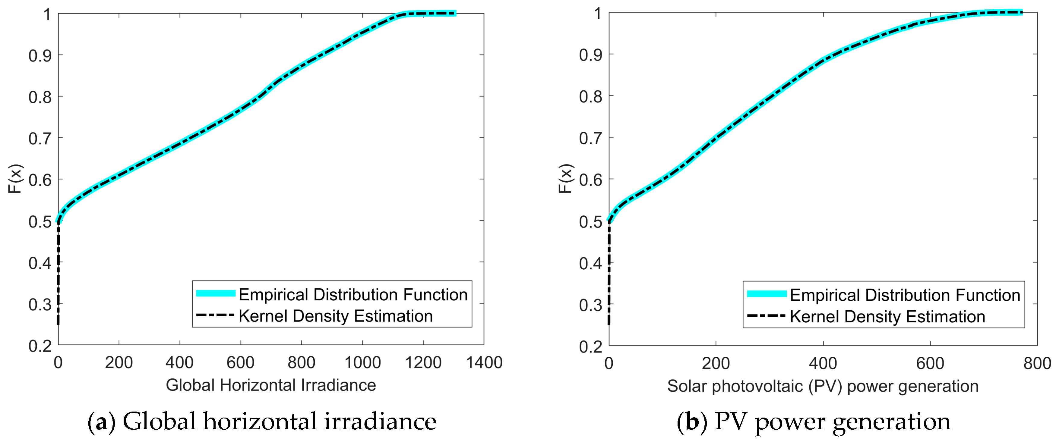
4.2. Correlation Analysis Based on Copula Function

There are many meteorological factors affecting photovoltaic power generation. Due to space limitations, this paper only presents the correlation analysis results of total horizontal radiation and photovoltaic power generation. To solve the Copula function, it is necessary to obtain the marginal distribution of the random variables, which can be obtained by parametric or non-parametric methods. This study used the non-parametric kernel density estimation method to process the data, and the obtained empirical distribution function and kernel distribution estimation are shown in Figure 3. Then, from the obtained kernel distribution estimation function, the marginal distribution of the random variables is calculated, and the parameters of the Copula function and its corresponding rank correlation coefficient are estimated from this marginal distribution estimation.

There are many commonly used Copula functions. This paper uses five commonly used Copula functions: Normal Copula, t-Copula, Gumbel Copula, Clayton Copula, and Frank Copula. Using them, we separately establish the joint distribution model of total horizontal radiation and photovoltaic power generation. Then, according to the marginal distribution, the maximum-likelihood estimation method is used to estimate the parameter values of the model. The obtained density function and distribution function are shown in Figure 4.

As can be seen in Figure 4, the joint density function of global horizontal radiation and photovoltaic power generation shows a symmetric tail. This indicates that when the value of global horizontal radiation is high, the photovoltaic power generation is also high, and vice versa. The distribution of global horizontal radiation and photovoltaic power generation is mainly concentrated on the 45° diagonal line, with two peaks at both ends of the diagonal line. The peak in the tail is higher, indicating that global horizontal radiation and photovoltaic power generation have a strong tail correlation. Their correlation is very obvious when the value of global horizontal radiation is high or low.

To further determine the optimal Copula function, we compare the squared Euclidean distance (SED) of each Copula function. The smaller the distance, the better the fit of the selected Copula function to the original data. The results are shown in

Table 2. SED for each Copula function.

Meteorological Factors	Normal Copula	t-Copula	Gumbel Copula	Clayton Copula	Frank Copula
Global horizontal radiation	148.3	112.9	175.4	132.1	48.79
Wind speed	39.20	23.25	71.28	28.19	9.558
Temperature	16.83	22.85	9.293	49.35	28.60
Wind direction	31.57	22.60	113.7	113.7	24.43
Max wind speed	55.99	35.69	89.80	47.12	13.05
Air pressure	18.44	23.49	33.30	33.30	18.59
pyranometer value	175.1	136.2	213.2	133.0	61.27
device temperature 1	27.12	17.03	24.53	127.5	13.93
device temperature 2	34.14	22.66	28.53	132.08	17.74

. As can be seen in Table 2, the SED of the Frank Copula for total horizontal radiation, wind speed, max wind speed, pyranometer value, device temperature 1, and device temperature 2 is the smallest. Therefore, the Frank Copula fits their original data correlation the best. The squared Euclidean distance of the Gumbel Copula for temperature is the smallest, the t-Copula for wind direction is the smallest, and the Normal Copula for air pressure is the smallest.

The correlation coefficients of each meteorological factor with photovoltaic power generation are shown in

Table 3. Kendall rank correlation coefficients and Spearman rank correlation coefficients for each feature.

Meteorological Factors	Kendall	Spearman
Global horizontal radiation	0.7269	0.9065
Wind speed	0.3577	0.5172
Temperature	0.3359	0.4801
Wind direction	−0.1649	−0.2405
Max wind speed	0.4128	0.5889
Air pressure	−0.1121	−0.1675
Pyranometer value	0.7168	0.8995
Device temperature 1	0.5559	0.7564
Device temperature 2	0.5538	0.7542

. The Spearman rank correlation coefficients of total horizontal radiation and the pyranometer value are 0.9065 and 0.8995, and the Kendall rank correlation coefficients are 0.7269 and 0.7168, so they have a strong positive correlation with photovoltaic power generation. The Spearman rank correlation coefficients of device temperature 1 and device temperature 2 are 0.7564 and 0.7542, and the Kendall rank correlation coefficients are 0.5559 and 0.5538. They are the temperatures of the photovoltaic device, and when the temperature is too high, it will affect the photovoltaic power generation.

The best meteorological factors selected by the model include total horizontal radiation, wind speed, temperature, maximum wind speed, pyranometer value, device temperature 1, and device temperature 2. The best meteorological factors are used as the input of the photovoltaic power generation prediction model.

4.3. Prediction Results with CA-Transformer

A total of 105,107 data samples were fed into the CA-Transformer network, and the network was trained using gradient descent to establish a photovoltaic power generation prediction model. For the CA-Transformer, the encoder part inputs data with indices 0–287 from a dataset, while the decoder part inputs data with indices 287–310. The established CA-Transformer photovoltaic power generation prediction model yielded an RMSE of 39.78, an MAE of 23.63, and an R² of 0.9512 for the test samples. The prediction effect of the photovoltaic power generation test samples is shown in Figure 5.

As can be seen in Figure 5, the model’s predicted values closely match the actual values, and the trends are generally consistent. This indicates that the CA-Transformer photovoltaic power generation prediction model can accurately predict the power generation trend under different weather conditions, demonstrating strong predictive and generalization capabilities. The first day is a typical sunny day with stable power generation changes, while the second and third days are typical cloudy days with varying degrees of load fluctuation. It can be seen that the prediction result for the first day is almost identical to the actual value, significantly better than the prediction results for the second and third days. This suggests that, compared to stable load change situations, the predictive ability of the CA-Transformer photovoltaic power generation prediction model decreases under load fluctuation and rapid change conditions, but it can generally adapt to these situations.

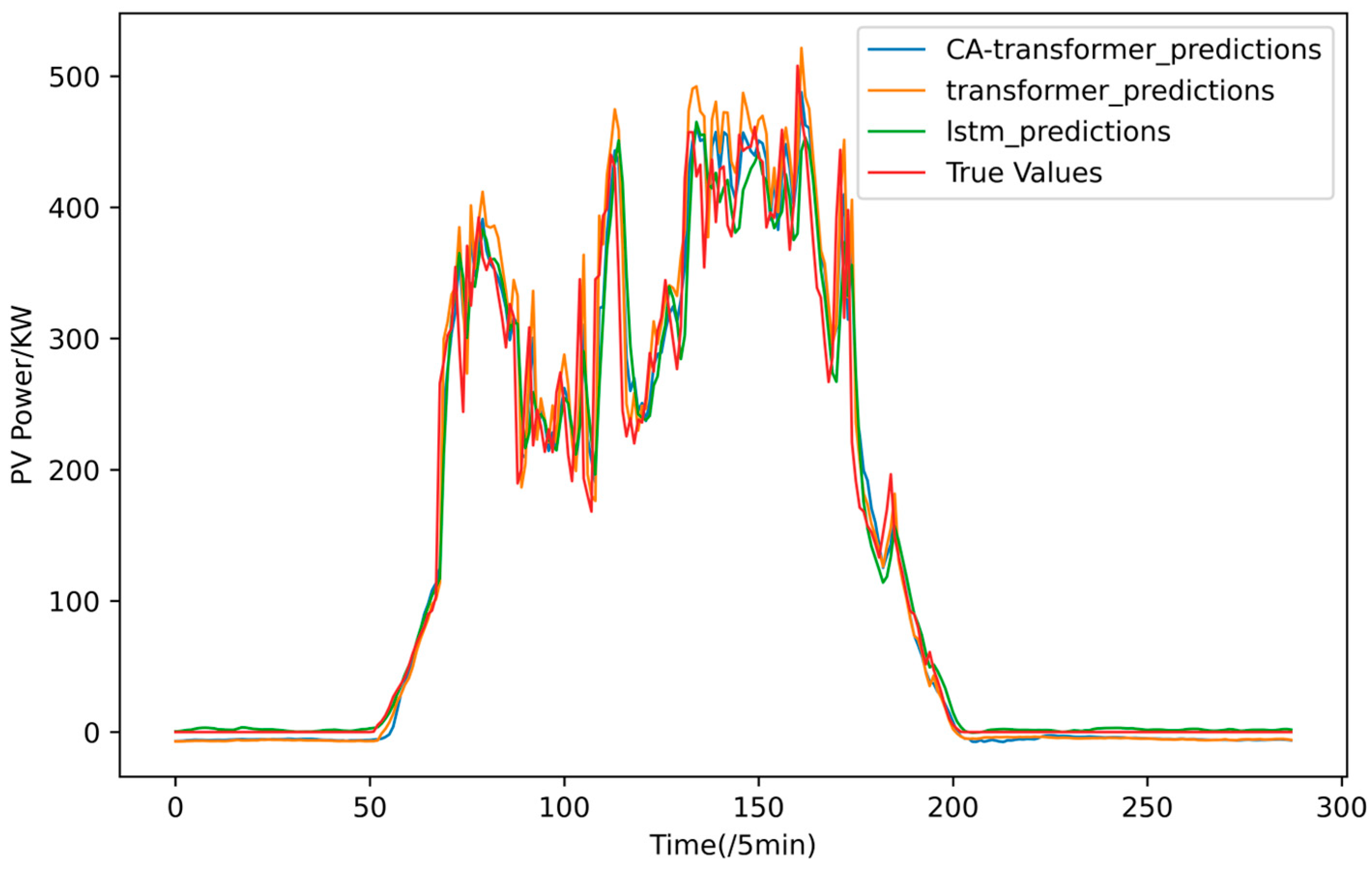
4.4. Comparison of Prediction Results

To further illustrate the predictive effect of the established photovoltaic power generation model based on the CA-Transformer, it is compared with models established based on LSTM and the Transformer. The RMSE, MAE, and R² were used to quantitatively evaluate the prediction effects of each model, and the prediction errors of the test samples are shown in

Table 4. Forecast results of different models.

Model	RMSE	MAE	R2
CA-Transformer	39.78	23.63	0.9512
Transformer	43.18	26.55	0.9426
LSTM	42.15	24.13	0.9453

.

From the data in Table 4, it can be seen that the prediction errors MSE and MAE of the established CA-Transformer photovoltaic power generation model are smaller than those of the models established based on LSTM and the Transformer, and the R2 is larger. This indicates that the model proposed in this paper has stronger predictive and generalization capabilities. The predictive effect of the CA-Transformer model is superior to that of the LSTM model, indicating that the CA-Transformer can effectively solve the gradient vanishing problem in long-sequence prediction, demonstrating strong predictive capabilities. The predictive effect of the CA-Transformer model is superior to that of the Transformer model, indicating that the CA-Transformer, by combining a CNN and cosine attention, enhances the model’s ability to learn photovoltaic power generation data features, demonstrating stronger advantages in photovoltaic power generation prediction. The prediction effects of different models are shown in Figure 6.

5. Conclusions

This paper proposes a photovoltaic power prediction model, CA-Transformer, based on the Copula function and reports on experiments conducted based on photovoltaic power generation and meteorological data. First, the Copula function is used to calculate the correlation coefficients between various meteorological factors and photovoltaic power generation. Meteorological factors with high correlations are selected according to their correlation coefficients. This feature selection provides a foundation for improving the prediction accuracy of the model. Furthermore, the experiment shows that the CA-Transformer, by combining the parallel structure of the 1D-RNN and the cosine self-attention module with the Transformer, fully utilizes the advantages of different models in processing time-series data and achieves significant improvements over both the Transformer and LSTM. Specifically, the RNN module captures the sequential dependencies of the data, while the cosine self-attention module enhances the extraction ability of global features. Ultimately, efficient integrated feature processing is achieved through the Transformer model.

In summary, the main contributions of this paper can be summarized as follows:

(1)

To establish a photovoltaic power generation prediction model, it is necessary to extract key meteorological factors that affect photovoltaic power generation. Common algorithms cannot comprehensively measure the nonlinearity and trend correlations between photovoltaic power generation and meteorological factors. This paper uses the Copula function to measure the nonlinear relationships and trend correlations between meteorological variables and photovoltaic power generation, which not only reduces the sample size but also improves prediction accuracy.

(2)

The combination of the RNN and cosine self-attention fully utilizes the advantages of both. The RNN is good at handling dependency relationships in sequential data, while cosine self-attention can better capture global information and long-distance dependencies. The self-attention mechanism uses cosine similarity instead of the dot product as the measure of self-attention, which can better capture similarities in time-series data. Finally, after integrating multiple feature representations and inputting them into the Transformer model, the powerful feature extraction and sequence processing capabilities of the Transformer can be fully utilized to further enhance prediction performance.

(3)

Through comparative experiments, the predictive performance of the proposed photovoltaic power prediction model, CA-Transformer, based on the Copula function is demonstrated, and the predictive performance is intuitively displayed, proving the effectiveness of the proposed method.

References

1. International Renewable Energy Agency. Available online: https://www.irena.org/Energy-Transition/Technology/Solar-energy (accessed on 20 February 2023).
2. International Energy Agency. Available online: https://www.iea.org/reports/solar-pv (accessed on 20 February 2023).
3. Zhou, Y. Artificial intelligence in renewable systems for transformation towards intelligent buildings. Energy AI 2022, 10, 100182. [Google Scholar] [CrossRef]
4. Al-Shetwi, A.Q.; Hannan, M.A.; Jern, K.P.; Mansur, M.; Mahlia, T.M.I. Grid-connected renewable energy sources: Review of the recent integration requirements and control methods. J. Clean. Prod. 2020, 253, 17. [Google Scholar] [CrossRef]
5. Blaga, R.; Sabadus, A.; Stefu, N.; Dughir, C.; Paulescu, M.; Badescu, V. A current perspective on the accuracy of incoming solar energy forecasting. Prog. Energy Combust. Sci. 2019, 70, 119–144. [Google Scholar] [CrossRef]
6. Viscondi, G.D.; Alves-Souza, S.N. A Systematic Literature Review on big data for solar photovoltaic electricity generation forecasting. Sustain. Energy Technol. Assess. 2019, 31, 54–63. [Google Scholar] [CrossRef]
7. Sobri, S.; Koohi-Kamali, S.; Abd Rahim, N. Solar photovoltaic generation forecasting methods: A review. Energy Convers. Manag. 2018, 156, 459–497. [Google Scholar] [CrossRef]
8. Wang, F.; Lu, X.X.; Mei, S.W.; Su, Y.; Zhen, Z.; Zou, Z.B.; Zhang, X.M.; Yin, R.; Dui, N.; Khah, M.S.; et al. A satellite image data based ultra-short-term solar PV power forecasting method considering cloud information from neighboring plant. Energy 2022, 238, 16. [Google Scholar] [CrossRef]
9. Markovics, D.; Mayer, M.J. Comparison of machine learning methods for photovoltaic power forecasting based on numerical weather prediction. Renew. Sustain. Energy Rev. 2022, 161, 17. [Google Scholar] [CrossRef]
10. Korkmaz, D. SolarNet: A hybrid reliable model based on convolutional neural network and variational mode decomposition for hourly photovoltaic power forecasting. Appl. Energy 2021, 300, 20. [Google Scholar] [CrossRef]
11. VanDeventer, W.; Jamei, E.; Thirunavukkarasu, G.S.; Seyedmahmoudian, M.; Soon, T.K.; Horan, B.; Mekhilef, S.; Stojcevski, A. Short-term PV power forecasting using hybrid GASVM technique. Renew. Energy 2019, 140, 367–379. [Google Scholar] [CrossRef]
12. Lima, M.; Carvalho, P.C.M.; Fernández-Ramírez, L.M.; Braga, A.P.S. Improving solar forecasting using Deep Learning and Portfolio Theory integration. Energy 2020, 195, 14. [Google Scholar] [CrossRef]
13. Lopes, F.M.; Silva, H.G.; Salgado, R.; Cavaco, A.; Canhoto, P.; Collares-Pereira, M. Short-term forecasts of GHI and DNI for solar energy systems operation: Assessment of the ECMWF integrated forecasting system in southern Portugal. Sol. Energy 2018, 170, 14–30. [Google Scholar] [CrossRef]
14. Sweeney, C.; Bessa, R.J.; Browell, J.; Pinson, P. The future of forecasting for renewable energy. Wiley Interdiscip. Rev. Energy Environ. 2020, 9, 18. [Google Scholar] [CrossRef]
15. Halabi, L.M.; Mekhilef, S.; Hossain, M. Performance evaluation of hybrid adaptive neuro-fuzzy inference system models for predicting monthly global solar radiation. Appl. Energy 2018, 213, 247–261. [Google Scholar] [CrossRef]
16. Hou, W.; Xiao, J.; Niu, L. Analysis of power generation capacity of photovoltaic power. Electr. Eng. 2016, 17, 53–58. [Google Scholar]
17. Miao, S.; Ning, G.; Gu, Y.; Yan, J.; Ma, B. Markov Chain model for solar farm generation and its application to generation performance evaluation. J. Clean. Prod. 2018, 186, 905–917. [Google Scholar] [CrossRef]
18. Massidda, L.; Marrocu, M. Use of Multilinear Adaptive Regression Splines and numerical weather prediction to forecast the power output of a PV plant in Borkum, Germany. Sol. Energy 2017, 146, 141–149. [Google Scholar] [CrossRef]
19. Agoua, X.G.; Girard, R.; Kariniotakis, G. Short-Term Spatio-Temporal Forecasting of Photovoltaic Power Production. IEEE Trans. Sustain. Energy 2018, 9, 538–546. [Google Scholar] [CrossRef]
20. Ibrahim, M.S.; Dong, W.; Yang, Q. Machine learning driven smart electric power systems: Current trends and new perspectives. Appl. Energy 2020, 272, 19. [Google Scholar] [CrossRef]
21. Hossain, M.; Mekhilef, S.; Danesh, M.; Olatomiwa, L.; Shamshirband, S. Application of extreme learning machine for short term output power forecasting of three grid-connected PV systems. J. Clean. Prod. 2017, 167, 395–405. [Google Scholar] [CrossRef]
22. Tso, G.K.F.; Yau, K.K.W. Predicting electricity energy consumption: A comparison of regression analysis, decision tree and neural networks. Energy 2007, 32, 1761–1768. [Google Scholar] [CrossRef]
23. Barman, M.; Choudhury, N.B.D. Season specific approach for short-term load forecasting based on hybrid FA-SVM and similarity concept. Energy 2019, 174, 886–896. [Google Scholar] [CrossRef]
24. Massaoudi, M.; Chihi, I.; Sidhom, L.; Trabelsi, M.; Refaat, S.S.; Oueslati, F.S. Enhanced Random Forest Model for Robust Short-Term Photovoltaic Power Forecasting Using Weather Measurements. Energies 2021, 14, 3992. [Google Scholar] [CrossRef]
25. Niu, D.X.; Wang, K.K.; Sun, L.J.; Wu, J.; Xu, X.M. Short-term photovoltaic power generation forecasting based on random forest feature selection and CEEMD: A case study. Appl. Soft Comput. 2020, 93, 14. [Google Scholar] [CrossRef]
26. Antonanzas, J.; Pozo-Vázquez, D.; Fernandez-Jimenez, L.A.; Martinez-de-Pison, F.J. The value of day-ahead forecasting for photovoltaics in the Spanish electricity market. Sol. Energy 2017, 158, 140–146. [Google Scholar] [CrossRef]
27. Voyant, C.; Notton, G.; Kalogirou, S.; Nivet, M.L.; Paoli, C.; Motte, F.; Fouilloy, A. Machine learning methods for solar radiation forecasting: A review. Renew. Energy 2017, 105, 569–582. [Google Scholar] [CrossRef]
28. Schmidhuber, J. Deep learning in neural networks: An overview. Neural Netw. 2015, 61, 85–117. [Google Scholar] [CrossRef] [PubMed]
29. Gao, M.; Li, J.; Hong, F.; Long, D. Day-ahead power forecasting in a large-scale photovoltaic plant based on weather classification using LSTM. Energy 2019, 187, 115838. [Google Scholar] [CrossRef]
30. Agga, A.; Abbou, A.; Labbadi, M.; El Houm, Y. Short-term self consumption PV plant power production forecasts based on hybrid CNN-LSTM, ConvLSTM models. Renew. Energy 2021, 177, 101–112. [Google Scholar] [CrossRef]
31. Dai, Y.; Wang, Y.; Leng, M.; Yang, X.; Zhou, Q. LOWESS smoothing and Random Forest based GRU model: A short-term photovoltaic power generation forecasting method. Energy 2022, 256, 124661. [Google Scholar] [CrossRef]
32. Zhen, H.; Niu, D.; Wang, K.; Shi, Y.; Ji, Z.; Xu, X. Photovoltaic power forecasting based on GA improved Bi-LSTM in microgrid without meteorological information. Energy 2021, 231, 120908. [Google Scholar] [CrossRef]
33. Vaswani, A.; Shazeer, N.; Parmar, N.; Uszkoreit, J.; Jones, L.; Gomez, A.N.; Kaiser, Ł.; Polosukhin, I. Attention is all you need. Adv. Neural Inf. Process. Syst. 2017, 30, 5999. [Google Scholar]
34. Zhao, Z.; Xia, C.; Chi, L.; Chang, X.; Li, W.; Yang, T.; Zomaya, A.Y. Short-Term Load Forecasting Based on the Transformer Model. Information 2021, 12, 516. [Google Scholar] [CrossRef]
Figure 1. The typical structure of a CNN.
Sustainability 16 05940 g001
Figure 2. CA-Transformer model architecture.
Sustainability 16 05940 g002
Figure 3. Nuclear distribution estimation and empirical distribution function of global horizontal irradiance and PV power generation.
Sustainability 16 05940 g003
Figure 4. Joint distribution model based on the Frank-Copula function.
Sustainability 16 05940 g004
Figure 5. CA-Transformer prediction results.
Sustainability 16 05940 g005
Figure 6. Predictions from different models.
Sustainability 16 05940 g006