Enhancing Environmental Sustainability: Risk Assessment and Management Strategies for Urban Light Pollution

Abstract

Light pollution imposes significant and far-reaching adverse effects on human society, necessitating its stringent regulation. However, intervention policies could be customized to suit the unique characteristics of each region, taking into account local conditions. To address this challenge, we have developed a comprehensive light pollution risk assessment model using a combination of objective and subjective weighting methods, including analytic hierarchy process (AHP), independent weighting method (IWM), entropy weight method (EWM), coefficient of variation (CV), criteria importance through intercriteria correlation (CRITIC), and principal component analysis (PCA). This model facilitates a systematic evaluation of light pollution risk levels across diverse regions in China. Subsequently, we have proposed intervention policies targeting light pollution risk reduction and assessed their efficacy using the synthetic control method. Our findings reveal elevated light pollution risk levels in coastal and mountainous regions with heightened concentrations closer to urban centers. Strategies focused on enhancing lighting hardware, optimizing lighting schedules, and upgrading light sources demonstrated the impact on reducing light pollution risk levels (LPRL). This study not only lays a solid theoretical foundation for assessing urban light pollution risks but furnishes empirical evidence to aid relevant authorities in formulating effective light pollution control strategies.

1. Introduction

Artificial light sources serve as an indispensable resource for humanity, providing today’s society with unparalleled flexibility by disconnecting human activities from the natural light cycle. This extension of activities into the night and the facilitation of indoor spaces lacking sufficient natural light during the day are contributions of artificial lighting. Over the course of history, numerous technological advancements have made the production and control of light increasingly achievable [1], a trend that has accelerated in recent centuries [2,3]. Presently, the widespread availability of artificial light is a cornerstone of many societies [4], with its pervasive use so ingrained that lighting has evolved into an “invisible infrastructure” [5,6]. While essential to daily life, lighting often goes unnoticed until its absence is felt.

Nevertheless, the excessive utilization of artificial light can yield detrimental effects. Light pollution obstructs people’s view of the night sky, impeding both modern astronomical discoveries [7] and ancient cultural traditions [8], and extends its impact to the well-being of humans, animals, and plants [9]. Artificial nighttime illumination disrupts human circadian rhythms, potentially leading to adverse health outcomes such as depression, obesity, and cancer [10]. Speculations abound that future perspectives might classify nocturnal artificial light as a human toxin akin to tobacco or asbestos [11]. Wildlife faces challenges, including restricted movement [12], circadian rhythm disruption [13], and reproductive disturbances [14]. Additionally, plant life is not spared, as the adverse effects of electric lights near vegetation are well-documented [15]. Studies suggest that the delicate equilibrium of ecosystems is in jeopardy due to nocturnal artificial lighting [16].

Artificial light presents a dual impact on communities across different regions, manifesting through diverse pathways. Efforts to reduce light pollution may inadvertently lead to increased local crime rates. The interplay of factors such as community development levels, population density, biodiversity, geography, and climate all contribute to the complexities of light pollution. Thus, the assessment of light pollution hazards and the formulation of intervention strategies should be carefully tailored to the specific local context. Robust assessment models are beneficial to empowering governments, urban planners, and environmental organizations to gain insights into the distribution, trends, and potential risks associated with light pollution. Through informed assessments, stakeholders can devise apt policies and interventions to effectively mitigate its adverse impact.

This paper aims to present a holistic light pollution hazard assessment model that amalgamates diverse environmental factors and data sources to enrich precise evaluations of light pollution hazards. The discussion will encompass the model’s design, outcomes, and its efficacy in practical applications. Through research and the development of the light pollution hazard assessment model, we aspire to deepen our comprehension of the ramifications of light pollution and enact more tailored interventions to safeguard our environment. This endeavor is to yield a substantial contribution towards addressing light pollution challenges and fostering sustainable urban development and ecological conservation.

The paper follows a structured outline beginning with Section 2, which covers the background and pertinent foundations. Section 3 elucidates the materials and methodology employed in the study. In Section 4, the analytical findings are presented, followed by the exploration of potentials and discussions in Section 5. Finally, Section 6 encapsulates the paper with conclusive remarks.

2. Literature Review

2.1. Strategy Development on Light Pollution Prevention

With the advancement of economic development, urban lighting systems have progressively evolved [17]. International entities like the World Health Organization advocate for the “One Health” concept, which seeks to sustainably enhance the well-being of humans, animals, and the environment through coordinated advancements [18]. While urban lighting endeavors contribute to creating aesthetically pleasing nightscapes for residents, they also engender a plethora of adverse effects. Principal manifestations of urban light pollution include atmospheric light pollution, glare, and light trespass [19]. Studies indicate that upwards of 80% of the global populace currently resides amidst nocturnal light pollution [20,21]. Excessive illumination disrupts the natural light rhythms of ecosystems, impacting the normal life cycles and development of humans and other organisms, thereby imperiling ecological equilibrium [22,23]. Research further reveals an alarming annual increase in light pollution rates, with Japan experiencing a 12% surge and European cities like Germany and Italy witnessing growth rates ranging from 6% to 10% [24].

Given this backdrop, numerous nations and international bodies have instituted measures to mitigate light pollution. The International Commission on Illumination (CIE) has issued a multitude of technical documents, with the most notable being the technical reports from CIE TC5 on light pollution research within lighting systems. The International Astronomical Union (IAU) oversees two committees dedicated to light pollution control: Commission 21 (The Light of the Night Sky) and Commission 50 (Protection of Existing and Potential Observatory Sites). In 1999, Commission 50 established a working group led by M. Smith, the director of Cerro Tololo Inter-American Observatory, to address light pollution concerns [25]. Subsequently, in 2000, this working group convened at the IAU meeting in Manchester, UK, to deliberate on the risks associated with light pollution [26].

2.2. Research on Risk Assessment Methods of Light Pollution

Liu et al. (2009) pioneered research on the risks associated with dynamic light changes [27]. Through dynamic simulations of the light environment, they extensively examined the impact of background brightness, distance, and stimulus levels on human sensory perceptions. Song et al. (2015) focused on nightscape lighting planning for main urban areas, employing a compound control index encompassing brightness zoning control, area development intensity, light–color zoning control, and energy-saving temporal control. This approach effectively aligned lighting with urban land use types and guided light pollution risk indicators [28]. Su and Hao (2012) developed 81 street facility lighting environment models by extracting environmental features. They defined the degree of light pollution risk and proposed a calculation formula for assessing light pollution infringement, laying a robust foundation for evaluating street light pollution in urban areas [29]. Feng et al. (2022) conducted extensive research on light pollution risk indicators and assessment methods, pioneering new directions in light pollution research by examining urban lighting evolution characteristics and utilizing VIIRS satellite images [30]. Advanced prediction algorithms like the generalized regression neural network (IFOA-GRNN) model offer valuable insights for light pollution research. Online education platforms can be leveraged to educate community residents. The conjoint analysis method, in conjunction with questionnaire surveys and expert interviews, was employed to specify the evaluation index system for light pollution. Ultimately, by integrating geographical elements, humanistic indicators, and direct impact factors, a structural equation of the influence index was established, providing a foundation for future research endeavors [31,32,33,34].

Dhanalakshmi and Radha (2022) [35] proposed an IoT-based system for monitoring and controlling air pollution in a cloud computing environment [36]. They introduced a linear regression and multi-class support vector (LR-MSV) method for air pollution prediction using IoT to monitor air quality data and air quality index measurements. Extensive experiments on an Indian dataset demonstrated the LR-MSV method’s excellent performance in prediction and error rate [37]. Liu and Mostafavi (2023) proposed a GIS and multi-criteria decision analysis (MCDA) method to address the challenge of integrating multiple factors in pollution risk assessments [38]. Messier and Katzfuss (2020) precisely mapped the spatial distribution of pollution sources using GIS technology and evaluated multiple influencing factors with MCDA, improving the accuracy and reliability of pollution risk assessments [39].

In summary, two primary research directions have emerged for defining light pollution risks. One approach involves utilizing policies, satellite imagery, and other resources to extract and integrate relevant indicators, constructing risk assessment models from specific perspectives. The other direction employs mathematical models or geographic information mining to assess pollution risks, refining risk assessment standards based on the unique characteristics of different regions. Studies primarily consist of exploratory evaluations. Currently, there is a scarcity of examples that combine multiple policy indicators to quantify pollution risks and validate assessment results with field policies. This study aims to bridge this gap by integrating external policies and developing a multi-indicator light pollution risk assessment system.

2.3. Application of Combined Weighting Method and Synthetic Control Method

To develop a comprehensive light pollution risk assessment indicator system, we have constructed a detailed framework based on the current light pollution research literature. This framework integrates factors such as regional light indices, regional development levels, climate, and geographic environment. To enhance the accuracy of risk level assessments, we employed the combined weighting method. While research on using this method for light pollution risk assessment is limited, we drew insights from advancements in other types of risk assessments. Early studies focused on constructing evaluation systems based on factors such as urban planning, building types, and traffic road usage intensity. Subsequent research incorporated locational factors, such as distance to relevant facilities, in evaluations. Recent achievements consider sustainability, ecological benefits, and social factors. In weight allocation, the reasonable combination of subjective and objective weighting is important for multi-attribute decision-making. Subjective weighting methods include expert scoring, analytic hierarchy process (AHP), correlation matrix method, and ranking comparison method. Among these, AHP stands out for its ability to hierarchize complex problems and quantify qualitative issues, making it more suitable for practical system risk assessments. Objective weighting methods consist of principal component analysis, the entropy method, and the mean square deviation method. To ensure more reliable assessment results, this study refers to the combination weighting method constructed and used in enterprise performance evaluation, adopting a more reasonable objective correction of subjective weighting to determine indicator weights. The final results will be analyzed from six perspectives.

To date, quantitative research on the impact of urban light pollution policies remains limited. The main challenges include the absence of comprehensive urban light pollution assessment methods. In traditional policy impact assessments, the difference-in-difference (DID) method is commonly used, comparing policy pilot cities with non-pilot cities over the same period to explore policy impacts. However, this method requires finding two cities with similar development levels, urbanization processes, population densities, and opposite policy implementations. Additionally, other factors can influence research outcomes. For instance, during the implementation of urban light pollution control policies, complementary policies are often introduced to optimize infrastructure and facilities, complicating comparisons. Therefore, we opted for the synthetic control method, which addresses the limitations of the DID method. This method considers the characteristic differences between pilot cities and other cities, creating a virtual control group by weighting the indicators of cities with similar characteristics. By minimizing city differences and accounting for multiple policy interferences, this approach allows for a more accurate assessment of policy effects.

3. Materials and Methods

3.1. Model Construction

3.1.1. Light Pollution Risk Level Assessment Model

The negative impacts of artificial light differ significantly across regions, influenced by factors such as local development levels, ecological environments, geographic features, and climatic conditions [40]. Consequently, assessing light pollution risk levels necessitates the integration of multiple influencing factors to develop a meaningful evaluation model. However, there is a gap in the literature, regarding the evaluation of light pollution risk levels, leaving our assessment model without direct references from existing research. To address this, we conducted an extensive literature review on current light pollution studies. Our findings indicate that factors such as the Bortle Dark-Sky Scale [41], the Comprehensive Night-Time Light Index, regional development levels, duration of illumination [42], and wildlife habitats [43] all significantly influence light pollution risk levels. Based on these insights, we constructed relevant indicators to inform our model.

To establish a light pollution risk level assessment model (The following is referred to as LPRLA Model), we selected representative indicators from the literature that align with the requirements of our study, as detailed in

Table 1. Light pollution risk level assessment indexes.

Symbols	Impact Metrics
BDS	The Bortle Dark-Sky Scale
CNLI	Comprehensive Night-Time Light Index
S	Light Area Ratio
FRANLI	Relative Average Night-Time Light Index
LUD	Level of Urban Development
GRP	Gross Regional Product
POP	Population Size
AASD	Average Annual Sunshine Duration
WHA	Wildlife Habitat Area

.

BDS: Skyglow is an indicator of the overall light pollution in a region, representing the amount of light scattered into the atmosphere and creating a hazy glow above the area. It can be measured using the Bortle Scale. The Bortle Scale measures the quality (brightness) of the night sky at a specific location, categorizing it into nine levels, with level 9 representing the most extreme light pollution. This scale utilizes actual celestial observations to estimate the overall sky brightness, aiding amateur astronomers in understanding the darkness of specific observation sites.

CNLI: Generally, the Comprehensive Night-Time Light Index ($CNLI$) or Relative Average Night-Time Light Index ($I$) can effectively reflect the lighting characteristics of a region. $I$ can be calculated by constructing the following indicators [44]:

$$I=\frac{1}{\mathrm{N}\ast \mathrm{D}{\mathrm{N}}_{\mathrm{m}\mathrm{a}\mathrm{x}}}\sum _{\mathrm{i}=1}^{\mathrm{D}{\mathrm{N}}_{\mathrm{m}\mathrm{a}\mathrm{x}}}\mathrm{D}{\mathrm{N}}_{\mathrm{i}}{\mathrm{n}}_{\mathrm{i}}$$

(1)

$I$ combined with the definition of $\mathrm{S}$ (light area ratio) yields the $CNLI$ formula as follows:

$$\mathrm{S}=\frac{{\mathrm{S}}_{\mathrm{p}\mathrm{a}\mathrm{r}\mathrm{t}}}{{\mathrm{S}}_{\mathrm{t}\mathrm{o}\mathrm{t}\mathrm{a}\mathrm{l}}}=\frac{n}{\mathrm{N}}$$

(2)

$$CNLI=I\times S$$

(3)

where $\mathrm{D}{\mathrm{N}}_{\mathrm{i}}$ represents the radiance value of each pixel grid unit within the region. $n$ is the number of grids in the region, generally corresponding to the size of the regional division, and $N$ is the total number of grids in the study area. $\mathrm{D}{\mathrm{N}}_{\mathrm{i}}{\mathrm{n}}_{\mathrm{i}}$ is the $DN$ value for the $n$th grid with index $i$. ${\mathrm{S}}_{\mathrm{p}\mathrm{a}\mathrm{r}\mathrm{t}}$ is the area under the DN values from 1 to $\mathrm{D}{\mathrm{N}}_{\mathrm{m}\mathrm{a}\mathrm{x}}$, and ${\mathrm{S}}_{\mathrm{t}\mathrm{o}\mathrm{t}\mathrm{a}\mathrm{l}}$ is the total administrative area of the study area. This represents the ratio of the illuminated area to the total area of the region.

LUD: The level of regional development significantly influences the degree of light pollution risk. Light pollution, a byproduct of industrialization, primarily arises from household lighting, advertising signage, offices, factories, streetlights, and outdoor sports lighting [45]. The more prosperous an area’s economy and the higher the living standards of its inhabitants, the greater the light pollution tends to be. Regions with abundant electricity resources and high population density are particularly susceptible to light pollution. To assess the level of regional development and subsequently evaluate the light pollution risk, we refer to division rules based on GDP and population. Specifically, we use the concepts of gross regional product (GRP) and population (POP) as key indicators.

AASD: Regional differences in sunshine duration, influenced by geographical and climatic factors, also affect the level of light pollution risk. Sunshine duration is typically associated with geographical elements such as latitude, season, and altitude as well as climatic conditions, like weather patterns. For instance, regions at higher latitudes generally experience shorter sunshine durations, while those at higher altitudes tend to enjoy longer sunshine durations. Furthermore, regions with more clear days throughout the year typically have extended periods of sunshine. These variations in sunshine duration directly impact the extent of artificial lighting required, thereby influencing the overall level of light pollution in different regions. We quantified this factor using the total monthly sunshine hours (unit: h) for various cities as reported in the “China Statistical Yearbook.”

WHA: We believe that the area of wildlife habitats can serve as an indicator for assessing the level of risk in areas with high light pollution. Light pollution can adversely affect wildlife in various ways, including disrupting circadian rhythms, altering migration patterns, and interfering with reproductive behaviors. These disruptions can significantly impact the behavior and health of wildlife populations. Hence, monitoring the extent of wildlife habitats and understanding the effects of light pollution on these areas are essential for comprehensive risk assessments [46]. Considering data availability and interpretability, we chose to use the area of nature reserves in each city as the quantification standard for the range of wildlife habitats.

3.1.2. Light Pollution Risk Intervention Strategy Model

Based on the Light Pollution Risk Level Assessment Model, we propose five corresponding intervention policies: reducing lighting time (RLT), improving light sources (ILS), enhancing lighting hardware (LIH), implementing greening projects (IGP), and enhancing light pollution community education (ECE). We assume that each policy exerts an equal impact on the indicators within the light pollution risk level assessment model. The specific policy actions and their relationships with the indicators are detailed as follows:

Reducing Lighting Time (RLT): In urban and peri-urban areas, communities can implement curfews to ensure that unnecessary outdoor lighting is turned off after a certain time at night, thereby reducing energy usage and costs. Community regulations should encourage the use of techniques such as shielding and directional lighting to optimize outdoor lighting practices. In regions distant from urban centers, specific areas can be designated for strict light pollution control to protect the night environment and minimize the negative impacts of light pollution on wildlife and human health. The implementation of this policy can effectively reduce the duration of lighting, as measured by average annual sunshine duration (AASD).

Improving Light Sources (ILS): Utilizing light waves that are less likely to cause light pollution can significantly reduce the harmful effects of light sources on living organisms. Lighting should employ directional illumination to precisely target areas that need light, minimizing reflections and limiting the range of intense light exposure. Encouraging the use of enclosed, fixed light sources can further promote the implementation of directional lighting. Additionally, lowering the threshold of lighting intensity helps to reduce sky glow and light intrusion. Implementing this policy can effectively decrease the sky glow index (BDS).

Improving Lighting Hardware (LIH): Shielding lighting fixtures can prevent upward-directed light, thereby reducing sky glow. Selecting appropriate lighting angles minimizes light pollution and decreases energy consumption and costs. Encouraging the use of energy-saving technologies—such as high-power or LED lighting and promoting new energy-efficient light sources—can further enhance these benefits. Outdoor lighting should utilize luminaires that meet dark sky standards, such as cutoff luminaires, to ensure minimal light emission from fixtures. Implementing this policy can result in significant improvements in the Comprehensive Nighttime Light Index (CNLI).

Implementing Greening Projects (IGP): Implementing greening projects can significantly improve wildlife habitats. Measures such as tree planting, vegetation restoration, and the construction of wetland parks can provide additional food sources and habitat space, attracting more wildlife for habitation and reproduction [47]. These initiatives improve the ecological environment, enhance biodiversity, and promote the balance and stability of ecosystems. The implementation of this policy can effectively increase the wildlife habitat area (WHA).

Enhancing Light Pollution Community Education (ECE): Strengthening community education on the hazards of light pollution and its mitigation is essential for raising environmental awareness. By educating the public, we can encourage the reduction of household and industrial lighting, especially in economically developed and densely populated areas. This proactive approach helps to reduce light pollution at the source, thereby mitigating associated risks [48]. The higher the level of regional development (LUD), the more urgently this policy is needed.

Based on the relationship between intervention policies and indicators, we can assume that the higher the correlation between an indicator and the light pollution risk level (the following is referred to as LPRL), the more effective the corresponding strategy implementation will be. Therefore, we will conduct correlation analysis between the relevant indicators and the LPRL scores from the light pollution risk assessment model. This analysis will help us identify and select intervention policies that demonstrate strong correlations with the LPRL and yield better implementation results.

After selecting the optimal intervention policies, we need to test their effectiveness. To evaluate the policy effects more intuitively and effectively, we will cluster all 370 prefecture-level cities in China based on light pollution risk assessment indicators, categorizing them into four types of regions (

Table 2. Four cluster categories.

Symbol	Definition
PL	Protected land
RC	Rural community
SC	Suburban community
UC	Urban community

):

To select more referential and applicable rural communities (RC) and suburban communities (SC), we choose one representative city for each category. Given that Changchun and Xi’an in China have already implemented relevant intervention strategies, we selected these two cities as sample locations to test the effectiveness of the policies.

The synthetic control method can evaluate the changes in the observed factor, LPRL, under conditions of implementing and not implementing the strategies, thereby testing the effectiveness of policy implementation. An exogenous policy shock divides the sample into two groups: the treat group, which receives the policy intervention, and the control group, which does not. Typically, several control groups (regions or cities not affected by the policy) are selected and combined through weighted averaging or an appropriate linear combination to create a synthetic control group. This synthetic control group is more credible than a subjectively selected control group [49]. To ensure more reasonable and accurate results, we combine cities within the same category that are not affected by the policy into one control group, further minimizing the impact of regional differences.

3.2. Data Description

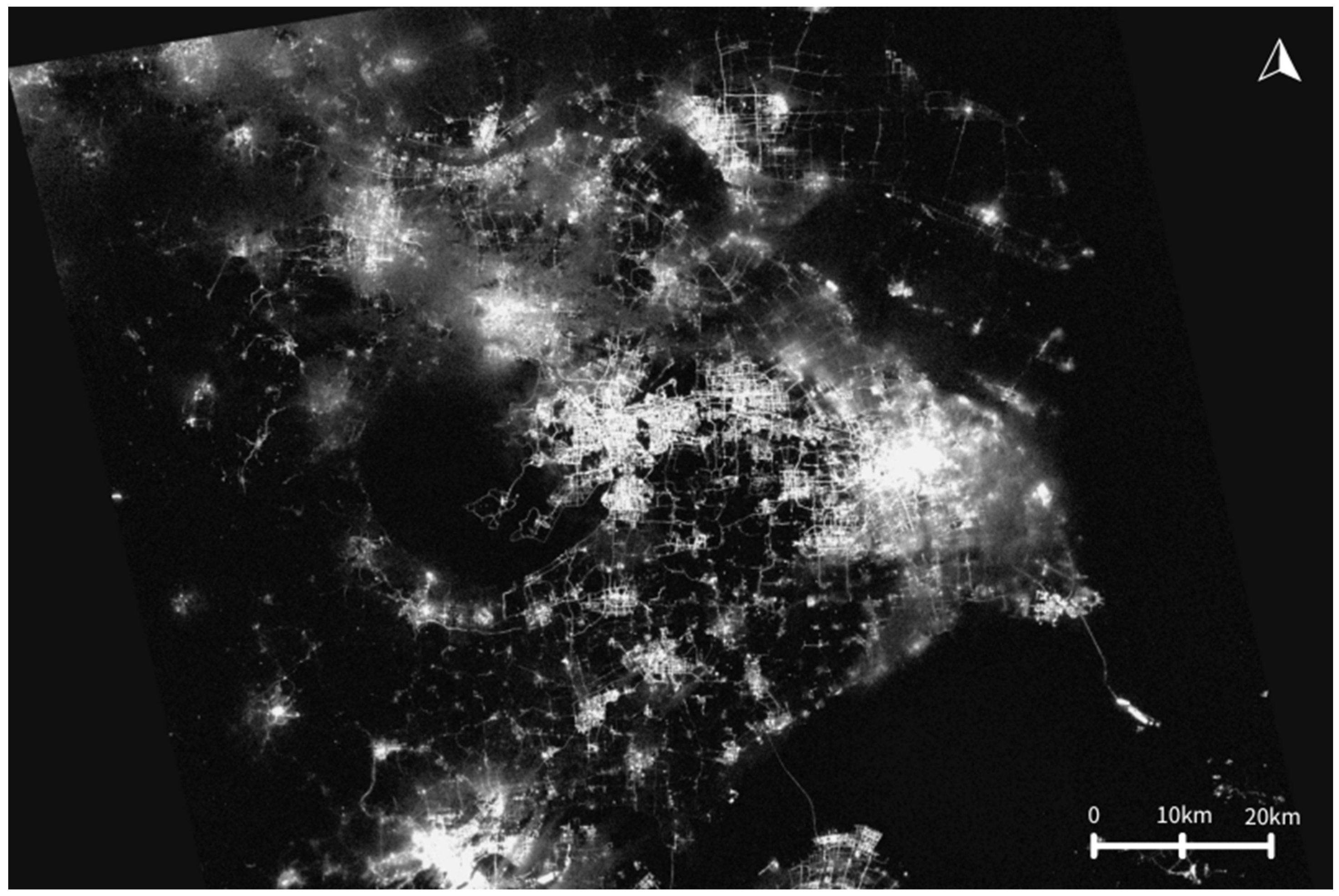
3.2.1. Data Sources

We collected images and corresponding data by region from the official Luojia-1 data website. Luojia-1 is the world’s first professional nighttime light remote sensing satellite, developed and produced by a team from Wuhan University in collaboration with relevant institutions. It was successfully launched on 2 June 2018. The satellite has a spatial resolution of 130 m and a swath width of 250 km by 250 km. Under ideal conditions, it can acquire and map global nighttime light imagery data every 15 days [50]. The product’s radiance conversion formula is as follows, where $L$ is the radiance value after absolute radiometric correction, measured in units

$$\mathrm{W}/\left({\mathrm{m}}^2\cdot \mathrm{s}\mathrm{r}\cdot \mathsf{\mu }\mathrm{m}\right)$$

(4)

and $dN$ is the image grayscale value.

$$L=d{N}^{\frac{3}{2}}\cdot {10}^{-10}$$

(5)

The screenshots of the official website interface and the obtained images are shown below.

In addition to the aforementioned image data, we also obtained relevant data and parameters from various other sources, including the 2022 China Statistical Yearbook, the Darkmap official website, and the Meteorological Bureau.

Figure 1 was taken by the Luojia-1 satellite (LJ1-01) in Wuhan at 14:15:27 on 29 October 2023. The image covers latitude and longitude from the upper left corner (121.635472, 32.570422) to the lower right corner (119.522701, 29.953885), and the center of the scene (120.558451, 31.25803). The product type is GEC System Geometry Correction product, and the file size is 15 MB. The sensor type used is CMOS, the product resolution is 130 m, the positioning accuracy is 82 m, and the image width and height are 2048 pixels. The image is named LuoJia1-01_LR202310307614_20231029141539_HDR_0023.

This image shows the ability of using high-resolution remote sensing technology to observe the surface under night conditions, providing important data support for urban lighting, population distribution, economic activities, and other studies.

3.2.2. Data Processing

For data processing and selection, we utilized ArcGIS to identify images and obtain numerical values of the nighttime light index. Additionally, we processed other data files, removing missing values and normalizing and standardizing the data. This scaling to a range within [0, 1] helps eliminate differences in magnitudes between various indicators, ensuring a balanced impact of each indicator on the model [51].

3.3. The LPRLA Model Based on Comprehensive Evaluation Method

The comprehensive evaluation method is a systematic and objective assessment based on relevant information. Indicator weighting is essential in the comprehensive evaluation of multiple indicators [52]. When individual indicators are fixed, changes in weights inevitably lead to changes in evaluation conclusions. Numerous weighting methods are used both domestically and internationally, including subjective and objective approaches.

Subjective weighting methods, which were studied earlier and are more mature, determine attribute weights based on the subjective importance assigned by decision-makers or experts. The original data are obtained subjectively by experts based on their experience using methods such as the analytic hierarchy process (AHP), which has passed consistency tests in this study.

Objective weighting methods, on the other hand, produce judgments independent of human subjectivity and have a strong mathematical theoretical basis. Examples include the independent weighting method (IWM), the entropy weighted method (EWM), coefficient of variation (CV), criterion importance through intercriteria correlation (CRITIC), and principal component analysis (PCA).

Among the various weighting methods, there is no absolutely correct or definitive measurement. Generally, the weights obtained by a specific weighting method under a given evaluation model are considered reasonable. Additionally, the selection of a particular method inherently involves subjectivity. When combining weights, it is advisable to select several methods from both information-based and subjective-objective weighting methods for combined analysis. Considering the advantages and disadvantages of subjective and objective weighting methods, this study refers to the combination weighting method used in enterprise performance evaluation to assess the level of light pollution risk.

3.3.1. Basic Weighting Method

The idea of combinatorial weighting in this paper is realized by integrating weights of various methods. Therefore, the optimal mathematical model is constructed to minimize the sum of squares of deviation between the weight vector of the combined method and the weight vector of each method, so as to determine the comprehensive weight of the evaluation index. Due to the variety of empowerment methods, and there is no absolute standard of excellence in practice, evaluators can only choose empowerment methods according to their own familiarity with empowerment methods and understanding of the importance of indicators. It is precisely because of the lack of uniform objective criteria that we cannot conclude that a certain empowerment outcome is more reasonable. Therefore, the weights obtained by different weighting methods can be weighted and averaged.

Each weighting method can be regarded as an estimate of the truth value of the index weight vector, and the combination of these weighting results can estimate the truth value more accurately. Therefore, in the absence of clear evidence that one weighting method is more effective than another, the subjective preferences of the evaluators should not be given too much consideration, nor should preference weights be added to the mix. Therefore, we employed various weighting methods, including AHP, IWM, EWM, CV, CRITIC, and PCA.

(1)

AHP is a multi-standard decision analysis method, which analyzes complex decision problems through hierarchical structure model and paired comparison so as to obtain the weight of each option. The root method is used to calculate the approximate value of the matrix eigenvector. AHP can combine the factors at different levels to form a multi-level analysis structure model based on the correlation and membership of the factors affecting the light pollution index, so this method is adopted. The calculation process is as follows:

Step 1: Calculate the nth root of the product of each row of elements of the judgment matrix A, the formula is as follows:

$${\mathrm{M}}_{\mathrm{i}}=\sqrt[\mathrm{n}]{\prod _{\mathrm{j}=1}^{\mathrm{n}}{\mathrm{a}}_{\mathrm{i}\mathrm{j}}}$$

(6)

Step 2: Normalize $M_i$, the formula is as follows:

$$Wi=\frac{M_i}{{\sum }_{i=1}^n{M}_i}$$

(7)

Step 3: Calculate the maximum eigenroot of the judgment matrix:

$$\lambda =\sum _{i=1}^n\frac{{\left(Aw\right)}_i}{n{w}_i}$$

(8)

(2)

IWM determines weights by analyzing the independence of indicators, calculates the correlation among indicators, reduces the influence of indicators with high correlation on weight distribution, and avoids the weight distortion caused by the interdependence of indicators. The method is an objective weighting method, which can extract data features more accurately.

The independent weight coefficient method is based on the collinearity between each index and other indicators to determine the weight of indicators. That is, if the multiple correlation coefficient $R$ between an indicator and other indicators is larger, the weight of the indicator is smaller.

$$R_j=\frac{{\sum }_{j=1}^m\left(x_j-\bar{x}\right)\left(\tilde{x}-\bar{x}\right)}{\sqrt{{\sum }_{j=1}^m{\left(x_j-\bar{x}\right)}^2{\left(\tilde{x}-\bar{x}\right)}^2}}\left(j=\mathrm{1,2},3,\dots ,m\right)$$

(9)

In the above equation, the reciprocal of the negative correlation coefficient is selected, and the final weight value is calculated after standardized processing:

$$W_j=\frac{\frac{1}{R_j}}{{\sum }_{j=1}^m\frac{1}{R_j}}$$

(10)

(3)

EWM uses information entropy to determine the weight of each indicator and obtain an objective weight allocation.

Step 1: Each factor is normalized according to the number of each option. For positive indicators:

$$z_{ij}=\frac{X_{ij}-X_{min}}{X_{max}-X_{min}}$$

(11)

For negative indicators:

$$z_{ij}=\frac{X_{max}-X_{ij}}{X_{max}-X_{min}}$$

(12)

Step 2: Calculate the entropy of the $j$th index

$$e_j=-k\sum _{i=1}^n{p}_{ij}ln\left(p_{ij}\right), j=1,\cdots ,$$

(13)

Step 3: Calculate the redundancy of information entropy (difference):

$$d_j=1-e_j, j=1,\cdots ,m$$

(14)

Step 4: Calculate the weights of each indicator:

$$w_j=\frac{d_j}{{\sum }_{j=1}^m{d}_j}, j=1,\cdots ,m$$

(15)

Step 5: Calculate the combined score of each sample:

$$s_i=\sum _{j=1}^m{w}_j{x}_{ij}, i=1,\cdots ,n$$

(16)

where $x_{ij}$ is the normalized data. According to the score of each influencing factor, the importance of all factors can be ranked.

(4)

CV is a statistical method that assigns weights by calculating the coefficient of variation of indicators. The greater the coefficient of variation, the higher the weight. The actual value of each variable is processed with data standardization, and then the weighted average method is adopted to determine the comprehensive score. The formula for calculating the coefficient of variation of each indicator is as follows:

$$V_i=\frac{{\sigma }_i}{X_i}$$

(17)

where: $V_i$ is the variation coefficient of item $i$; ${\sigma }_i$ is the standard deviation of item i; Xi is the arithmetic mean of item i. The formula for calculating the weight of each variable is as follows:

$$W_i=\frac{V_i}{{\sum }_{i=1}^n{V}_i}$$

(18)

(5)

CRITIC determines the weight of each indicator and reflects the relative importance of each indicator by analyzing the correlation and comparison strength of each indicator. For the CRITIC method, when the degree of positive correlation between the two indicators is greater, the conflict is smaller, which indicates that the information reflected by the two indicators in the evaluation of the pros and cons of the scheme is relatively similar.

Step 1: Determine the indicator variability. Expressed as standard deviation, $S_j$ represents the standard deviation of the JTH indicator.

$$\left\{\begin{array}{ll}{\bar{x}}_j=\frac{1}{n}{\displaystyle \sum _{i=1}^n}{x}_{ij}& \\ S_j=\sqrt{\frac{{\sum }_{i=1}^n{\left(x_{ij}-{\bar{x}}_j\right)}^2}{n-1}}& \end{array}\right.$$

(19)

The larger the standard deviation is, the greater the difference between the values of the indicator, the more information can be projected and the stronger the evaluation strength of the indicator itself, meaning more weight should be assigned to the indicator.

Step 2: Determine the indicator conflict. Expressed in the form of correlation coefficient, $r_{ij}$ represents the correlation coefficient between evaluation indicators $i$ and $j$.

$$R_j=\sum _{i=1}^p\left(1-r_{ij}\right)$$

(20)

The correlation coefficient is used to represent the correlation among indicators. The stronger the correlation is with other indicators, the smaller the conflict between the indicator and other indicators. The more the same information is reflected, the more repeated the evaluation content can be reflected. To some extent, the evaluation intensity of the indicator is weakened, and the weight assigned to the indicator should be reduced.

Step 3: Calculate the information. The larger the $C_j$ is, the greater the role of the JTH evaluation index in the whole evaluation index system, so more weight should be assigned to it.

$$C_j=S_j\sum _{i=1}^p\left(1-r_{ij}\right)=S_j\times R_j$$

(21)

Step 4: Calculate the weights. The objective weight of the JTH index is $W_j$.

$$W_j=\frac{C_j}{{\sum }_{j=1}^p{C}_j}$$

(22)

(6)

PCA converts high-dimensional data to low-dimensional data while retaining the maximum amount of information and determines the weight of each index by calculating the contribution rate of principal components.

The essence of PCA is to seek comprehensive replacement objects of related variables through the correlation of original variables and to ensure the minimum information loss in the transformation process. This is consistent with our multifactor model.

Step 1: Calculate the covariance matrix R based on the normalized data set:

$$R={\left(r_{ij}\right)}_{n\times n}=\left[\begin{array}{cccc}{r}_{11}& r_{12}& \cdots & r_{1n}\\ r_{21}& r_{22}& \cdots & r_{2n}\\ ⋮& ⋮& & ⋮\\ r_{n1}& r_{n2}& \cdots & r_{nn}\end{array}\right]$$

(23)

Step 2: Calculate the eigenvalues of matrix R and corresponding eigenvectors:

$$\left\{\begin{array}{l}{y}_1=u_{11}{\bar{x}}_1+u_{21}{\bar{x}}_2+\cdots +u_{n1}{\bar{x}}_n\\ y_2=u_{12}{\bar{x}}_1+u_{22}{\bar{x}}_2+\cdots +u_{n2}{\bar{x}}_n\\ y_n=u_{1w}{\bar{x}}_1+u_{2n}{\bar{x}}_2+\cdots +u_{nn}{\bar{x}}_{n^{*}}\end{array}\right.$$

(24)

where $y_1$ is the first principal component, $y_2$ is the second principal component, … $y_n$ is the $n$th principal component. Calculate the contribution rate of each principal component $y_1$ $b_j$ ($j$ = 1, 2, … $n$) and $y_1$, $y_2$, …, the cumulative contribution rate of $y_n$ ($p$ ≤ $n$) ${\alpha }_p$.

$$b_j=\frac{{\lambda }_j}{{\sum }_{k=1}^n{\lambda }_k} \left(j=\mathrm{1,2},\cdots ,n\right)$$

(25)

$${\alpha }_p=\frac{{\sum }_{k=1}^p{\lambda }_k}{{\sum }_{k=1}^n{\lambda }_k} \left(p\le n\right)$$

(26)

This method is adopted because each principal component is a linear combination of the original variables, independent of each other, and retains most of the information of the original variables, which greatly preserves the essential characteristics of the light pollution index.

3.3.2. Combined Weights

The combination weighting method integrates both the amount of information and subjective judgment. Several methods are selected for combined analysis from both the subjective and objective assignment approaches [53]. First, let the region Si evaluated by LPRL be measured by the jth indicator ${\mathrm{Q}}_{\mathrm{j}}$ to obtain Si’s indicator value of ${\mathrm{Q}}_{\mathrm{j}}$ as $a_{\mathrm{i}\mathrm{j}}$ (i ∈ N) (N = 1, 2… $n$), ($j$ ∈ M) (M = 1, 2… $m$) [54]. The normalization matrix R = (rij) n × m, and the weight vectors uk of each method $u_{\mathrm{k}}$ = ($u_{k1}$, $u_{k1}$… $u_{km}$), (k = 1, 2, … p). From these p weight vectors, the following combined weight vector matrix U is obtained.

$$\mathrm{U}=\left[\begin{array}{c}{u}_1\\ u_2\\ ⋮\\ u_p\end{array}\right]={\left[\begin{array}{cccc}{u}_{11}& u_{12}& \cdots & u_{1_m}\\ u_{21}& u_{22}& \cdots & u_{2_m}\\ ⋮& ⋮& ⋮& ⋮\\ u_{p}1& u_{p}2& \cdots & u_{pm}\end{array}\right]}_{p^{2}m}$$

(27)

Based on the principle that the deviation of evaluation results under subjective and objective assignment should be minimized, this paper introduces a deviation function and establishes the following weighted least squares superiority model for determining indicator weights.

$$\begin{array}{ll}& \mathrm{m}\mathrm{i}\mathrm{n} {\displaystyle \sum _{k=1}^p}{\displaystyle \sum _{i=1}^n}{\displaystyle \sum _{j=1}^m}{\alpha }_k{\left[\left(w_j-u_{kj}\right)r_{ij}\right]}^2\\ & \mathrm{s}.\mathrm{t}. {\displaystyle \sum _{j=1}^m}{w}_j=1,w_j>0\left(j\in \mathrm{M}\right)\end{array}$$

(28)

Based on the above indicators, we obtain the weight coefficients:

$$\begin{array}{c}{\displaystyle \sum _{j=1}^m}{u}_{ki}=1\end{array}$$

(29)

${\alpha }_k$ ($k$ = 1, 2, … p) are the weight coefficients of the p assignment methods and satisfy the following:

$$\begin{array}{c}{\displaystyle \sum _{k=1}^p}{\alpha }_i=1\end{array}$$

(30)

and construct the constructive Lagrangian function.

$$L\left(w,\lambda \right)=\sum _{k=1}^p\sum _{i=1}^n\sum _{j=1}^m{\alpha }_k{\left[\left(w_j-u_{ki}\right)r_{ij}\right]}^2+2\lambda \left(\sum _{j=1}^m{w}_j-1\right]$$

(31)

By taking partial derivatives of both sides of the above equation, the optimal solution of the model can be obtained from the necessary conditions for the existence of extreme values.

$$w_j=\sum _{k=1}^p{\alpha }_k{u}_{kj},j\in \mathrm{M}$$

(32)

We know the definition and properties of relative entropy, and details are as follows:

Definition 1.

Let xi, $y_i$ ≥ 0 (i = 1, 2 …n) and

$$\begin{array}{cc}{\displaystyle \sum _{\begin{array}{c}i=1\end{array}}^n}{x}_i& \ge {\displaystyle \sum _{i=1}^n}{y}_i\end{array}$$

(33)

Then, the relative entropy of x with respect to y is said to be as follows:

$$h\left(x,y\right)=\sum _{i=1}^n{x}_i\mathrm{l}\mathrm{o}\mathrm{g}\frac{x_i}{y_i}$$

(34)

Property 1.

Non-negativity of relative entropy.

Property 2.

A sufficient necessary condition for the relative entropy to be zero: $x_i$ = $y_i$ holds for all i.

From the relative entropy property, it is known that when xy is two discrete distributions, the relative entropy can measure the degree of conformity of the two. Determining αk involves determining the credibility of the kth weight vector, with αk serving as a quantitative representation of this credibility. This paper employs the following method to determine the credibility αk of the kth weighting result.

First, the relative entropy $h$ ($u_i$, $u_j$) between any two weight vectors $u_i$, $u_j$ ($i$, $j$ = 1, 2…$p$) is defined as follows.

$$h\left(u_i,u_j\right)=\sum _{l=1}^m{u}_{il}\mathrm{l}\mathrm{o}\mathrm{g}\frac{u_{il}}{u_{jl}}$$

(35)

The relative entropy $h$ ($u_i$, $u_j$) = 0 if and only if ∀l ∈ M, ∃$u_{il}$ = $u_{jl}$. Therefore, the relative entropy $h$ ($u_i$, $u_j$) can be used to measure the degree of conformity of the weight vectors $u_i$ and $u_j$, obtained by two different weighting methods. Based on the above principle, the problem of assembling weights $d$ = ($d_1$, $d_2$…$d_m$) can be transformed into the following mathematical programming problem.

$$\begin{gathered} \mathrm{m}\mathrm{i}\mathrm{n}H\left(d\right)=\sum _{j=1}^p\sum _{i=1}^m{d}_i\mathrm{l}\mathrm{o}\mathrm{g}\frac{d_i}{u_{ji}} \\ \mathrm{s}\cdot \mathrm{t}\cdot \sum _{i=1}^m{d}_i=1,d_i>0\left(i\in \mathrm{M}\right) \end{gathered}$$

(36)

The following theorem can be obtained for the optimization model of the above equation: the model has a global optimal solution $d^{*}$ = ($d_1^{*}$, $d_2^{*}$…$d_{\mathrm{m}}^{*}$), where

$$d_i^{*}=\frac{{\prod }_{i=1}^p{\left(u_{ji}\right)}^{\frac{1}{p}}}{{\sum }_{i=1}^m{\prod }_{j=1}^p{\left(u_{ji}\right)}^{\frac{1}{p}}} i=1,2\cdots ,m$$

(37)

The closeness $h$ ($u_i$, $d^{*}$) ($i$, $j$ = 1, 2…$p$) of each assignment result to the set weight $d^{*}$ = ($d_1^{*}$, $d_2^{*}$…$d_{\mathrm{m}}^{*}$) is calculated, and the credibility of each assignment result is calculated. The greater the closeness of the kth assignment result to the set weight vector, the greater its role in the combined assignment, and the credibility weight of this assignment result is shown as follows.

$${\alpha }_i=\frac{h\left(u_i,d^{*}\right)}{{\sum }_{i=1}^{p}h\left(u_i,d^{*}\right)} i=1,2,\cdots ,p$$

(38)

Finally, the confidence weights ${\alpha }_{\mathrm{k}}$ ($k$ = 1, 2, … $p$) are substituted into the formula to obtain the indicator combination weights $W_{\mathrm{j}}$ ($j$ ∈ M).

3.3.3. Weight Calculation

For the comprehensive assessment of light pollution risk levels, we utilized MATLAB R2018a software. Therefore, we employed various weighting methods, including AHP, IWM, EWM, CV, CRITIC, and PCA. The corresponding methods and indicators are outlined in

Table 3. Evaluation metric weights.

Empowerment Methods	BDS	CNLI	GRP	POP	AASD	WHA
AHP	0.1748	0.1569	0.1569	0.2190	0.1985	0.1351
IWM	0.1853	0.1592	0.1592	0.1413	0.1911	0.1848
EWM	0.0806	0.1192	0.1192	0.2863	0.1185	0.1320
CV	0.1073	0.1395	0.1395	0.2459	0.1304	0.1497
CRITIC	0.1204	0.1190	0.1190	0.1244	0.2602	0.2641
PCA	0.1596	0.1423	0.1423	0.2148	0.1279	0.1612

below.

We can get the combined weight vector matrix:

$$\mathrm{U}=\left[\begin{array}{c}{\mathrm{u}}_1\\ {\mathrm{u}}_2\\ {\mathrm{u}}_3\\ {\mathrm{u}}_4\\ {\mathrm{u}}_5\\ {\mathrm{u}}_6\end{array}\right]=\left[\begin{array}{cccccc}0.1748& 0.1569& 0.1157& 0.2190& 0.1985& 0.1351\\ 0.1853& 0.1592& 0.1383& 0.1413& 0.1911& 0.1848\\ 0.0806& 0.1192& 0.2634& 0.2863& 0.1185& 0.1320\\ 0.1073& 0.1395& 0.2272& 0.2459& 0.1304& 0.1497\\ 0.1204& 0.1190& 0.1119& 0.1244& 0.2602& 0.2641\\ 0.1596& 0.1423& 0.1942& 0.2148& 0.1279& 0.1612\end{array}\right]$$

(39)

The set weights of each indicator can be obtained (retaining four decimal places):

$$\begin{array}{cc}\hfill {\mathrm{W}}_{\mathrm{j}}& =\left({\mathrm{w}}_1,{\mathrm{w}}_2\dots {\mathrm{w}}_{\mathrm{m}}\right)\hfill \\ & =\left(0.1659,0.1660,0.1746,0.1699,0.1717,0.1627\right)\hfill \end{array}$$

(40)

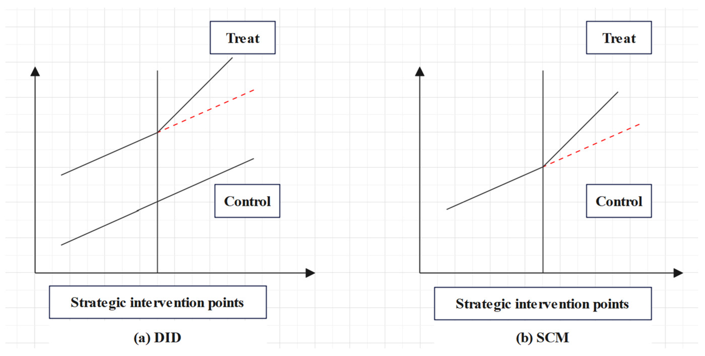
3.4. Model of Light Pollution Risk Intervention Strategies Based on the Synthetic Control Method

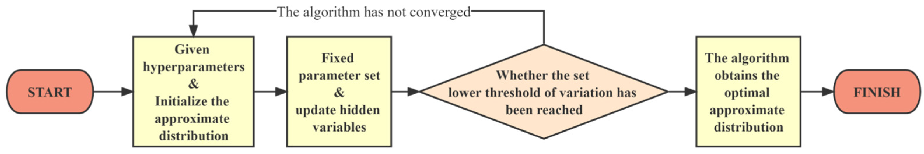
3.4.1. Gaussian Mixed Model

Gaussian mixed model (GMM) is a common clustering algorithm, similar to the K-means algorithm, and uses the EM (Expectation–Maximization) algorithm. The EM algorithm is an iterative process, which is for maximum likelihood estimation of parameters in probabilistic models containing hidden variables. GMM uses this algorithm to express the clustering prototype through a probabilistic model, ultimately obtaining the probabilities of each category [55]. The general flowchart for implementing the GMM algorithm is as follows (Figure 2):

We conducted Gaussian mixture model (GMM) clustering on a dataset comprising indicators from 370 prefecture-level cities, including BDS, CNLI, LUD, AADS, and WHA. In this model, we chose Euclidean distance for distance calculation with the following equation.

$$d\left(X,Y\right)=\sqrt{\sum {\left(x_i-y_i\right)}^2},\left(i=1,2,\dots ,n\right)$$

(41)

Step 1: Initialize the model parameters ${\alpha }_{\mathrm{i}}$, ${\mu }_i$ type, Σi for the mixed Gaussian distribution. The sample set D = {x1, x2…xm} is known, and we assume that the samples obey the mixed Gaussian distribution.

$${\mathrm{p}}_{\mathrm{M}}\left(\mathbf{x}\right)=\sum _{\mathrm{i}=1}^{\mathrm{k}}{\alpha }_{\mathrm{i}}\cdot \mathrm{p}\left(\mathrm{x}\mid {\mu }_i,{\mathsf{\Sigma }}_i\right)$$

(42)

$$\mathrm{p}\left(\mathrm{x}\mid {\mathsf{\mu }}_i,{\mathsf{\Sigma }}_i\right)=\frac{1}{{\left(2\pi \right)}^{\mathrm{n}/2}{\mathsf{\Sigma }}_j{|}^{1/2}}\mathrm{e}\mathrm{x}\mathrm{p}\left\{-\frac{1}{2}{\left(\mathrm{x}-{\mathsf{\mu }}_i\right)}^{\mathrm{T}}{\mathsf{\Sigma }}_i^{-1}\left(\mathrm{x}-{\mathsf{\mu }}_i\right)\right\}$$

(43)

The above equation is a multivariate Gaussian distribution, i.e., a mixture component. ${\alpha }_{\mathrm{i}}$ represents the mixing coefficient, i.e., the probability of selecting the $j$th mixture component. Satisfying the properties ${\alpha }_{\mathrm{i}}$ > 0, Σ${\alpha }_{\mathrm{i}}$ = 1, ${\mathsf{\mu }}_i$ represents the n-dimensional mean vector of each mixture component, and Σi represents the n × n covariance matrix.

Step 2: Compute the posterior probability ${\gamma }_{\mathrm{j}\mathrm{i}}$ of $x_j$ generated by each mixture component.

$${\gamma }_{\mathrm{j}\mathrm{i}}=\frac{{\alpha }_{\mathrm{i}}\cdot \mathrm{p}\left(x_j\mid {\mu }_i,{\Sigma }_i\right)}{{\sum }_{\mathrm{l}=1}^{\mathrm{k}}{\alpha }_l\cdot \mathrm{p}\left(x_j\mid {\mu }_l,{\Sigma }_l\right)}$$

(44)

Step 3: Compute the new model parameters.

$$\begin{array}{ll}& {\mu }_i^{\prime }=\frac{{\sum }_{\mathrm{j}=1}^{\mathrm{m}}{\gamma }_{\mathrm{j}\mathrm{i}}{\mathrm{x}}_{\mathrm{j}}}{{\sum }_{\mathrm{j}=1}^{\mathrm{m}}{\gamma }_{\mathrm{j}\mathrm{i}}}\\ & {\Sigma }_i^{\prime }=\frac{{\sum }_{\mathrm{j}=1}^{\mathrm{m}}{\gamma }_{\mathrm{j}\mathrm{i}}\left({\mathrm{x}}_{\mathrm{j}}-{{\mathsf{\mu }}_{\mathrm{i}}}^{\prime }\right){\left({\mathrm{x}}_{\mathrm{j}}-{{\mathsf{\mu }}_{\mathrm{i}}}^{\prime }\right)}^{\mathrm{T}}}{{\sum }_{\mathrm{j}=1}^{\mathrm{m}}{\gamma }_{\mathrm{j}\mathrm{i}}}\\ & {\alpha }_{\mathrm{i}}^{\prime }=\frac{{\sum }_{\mathrm{j}=1}^{\mathrm{m}}{\gamma }_{\mathrm{j}\mathrm{i}}}{\mathrm{m}}\end{array}$$

(45)

Step 4: Repeat Step 2 and Step 3 according to the new model parameters until the stopping condition is satisfied.

Step 5: Assign each sample to the corresponding cluster as follows: Each sample is assigned to the cluster of the sub-model with the highest probability, resulting in k clusters. Specifically, we divide the LPRL data set into four categories of cities according to indicators, in which cities with close indicators are in one category and cities with distant indicators are in different categories.

$${\lambda }_{\mathrm{j}}=\underset{\mathrm{i}\in \{1,2,\dots ,\mathrm{k}\}}{\mathrm{a}\mathrm{r}\mathrm{g}\mathrm{m}\mathrm{a}\mathrm{x}}{\gamma }_{\mathrm{j}\mathrm{i}}$$

(46)

We filter out the classification results according to the category sequence number and obtain the independent data set of four categories of cities, namely PL, RC, SC, UC.

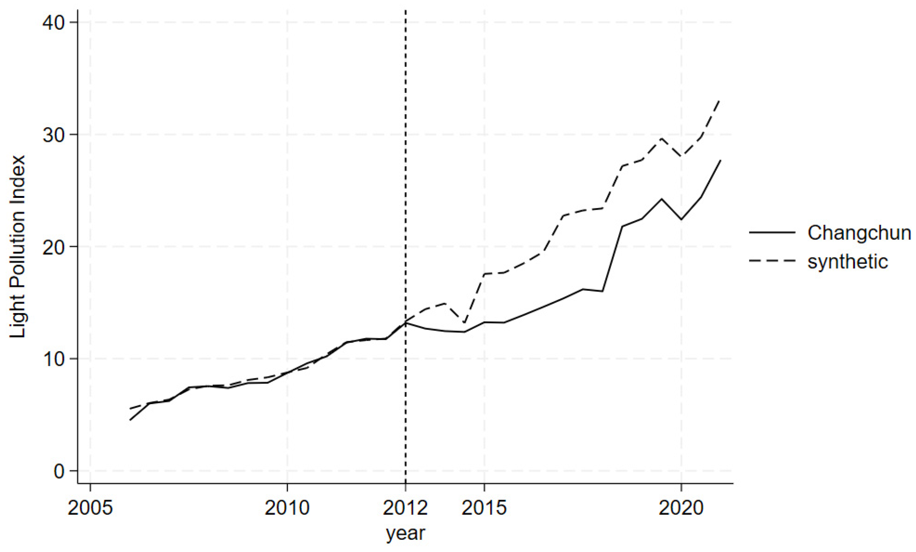
3.4.2. Synthetic Control Methods

The Synthetic control method (SCM) is a policy effectiveness assessment method proposed by Abdi and Greaseball. As a non-parametric method, SCM is an extension of the traditional differences-in-differences (DID) approach. The ideological differences between SCM and DID can be illustrated by the following diagram (Figure 3).

The synthetic control method (SCM) is primarily used for evaluating policy effects in sociology. Generally, SCM is applicable to panel data, combining both cross-sectional and time-series characteristics. Our test samples are therefore selected from Changchun for the years 2011 to 2019 (with policy implementation around 2015), covering 8 years, and from Xi’an for the years 2005 to 2019 (with policy implementation around 2012), covering 14 years. Cross-sectional data for each year were used as the analysis sample. Based on the model and data, we can make the following assumptions:

• Ignore the effects of the three strategies and other related policies.
• Disregard the impact of time differences in the implementation of policies in each city.
• Disregard the intensity changes of the three strategies themselves over time. Only one strategy implementation time point is considered.

After GMM clustering with Xi’an and Changchun in the same category but not using the policy of several control groups (not affected by the policy area, city), we weighted the average and produced a synthetic control group. This synthetic control group is more credible than the control group previously selected based on subjective selection, and it better overcomes the problem of differences between the treat and control groups.

It is assumed that there are ($1+J$) regions, where the first region is a disturbance strategy that reduces LPRL, while the remaining J regions are unshocked and constitute a potential control group. The weights of the synthetic control regions are noted as the following J-dimensional column vectors.

$$w={\left(w_1\dots w_{J+1}\right)}^{\prime }$$

(47)

where $w_i$ denotes the weight that the ith area occupies in this region. For the potential control group (donor pool) that is not affected by the policy, a weight value is given to each control area within the control group by the weight vector to form a synthetic control area. The elements of the weight vector are non-negative and sum to 1.

The average of the predictor variables of the treated areas before the policy intervention is recorded as vector ${\mathrm{X}}_1$. The average of the corresponding predictor variables of other potential control areas (where no relevant policy is implemented) is recorded as matrix ${\mathrm{X}}_0$ The weights w is chosen so that ${\mathrm{X}}_0$ is as close as possible to ${\mathrm{X}}_1$. In practice, we will put the Changchun and Xi’an areas into the model separately rather than both places into the same model.

$$X_0\cdot w=\left(x_1\dots x_{J+1}\right){\left(w_1\dots w_{J+1}\right)}^{\prime }=w_2{x}_2+\dots +w_{J+1}{x}_{J+1}\approx x_1$$

(48)

The solution for the optimal weights is modeled as follows: a weighted sum-of-squares minimization problem with constraints.

$$\begin{gathered} {\mathrm{m}\mathrm{i}\mathrm{n}}_w{\left(x_1-X_{0}w\right)}^{\prime }V\left(x_1-X_{0}w\right) \\ s.t.w_j\ge 0,j=2,\dots ,J+1;{\Sigma }_{j=2}^{J+1}{w}_j=1 \end{gathered}$$

(49)

where $V$ is a ($K$ × $K$) dimensional diagonal matrix whose diagonal elements are all non-negative weights, reflecting the corresponding predictor variables

For the relative importance of the explanatory variables, $Z_0{w}^{*}$($V$) is used to predict $z_1$. $V$ is chosen to minimize mean squared prediction error (MSPE), which means that the prediction error of each period is squared and averaged across periods. The objective function of this minimization problem is quadratic, which is a quadratic programming problem. Solving the minimization problem below yields the optimal weights that constitute the area where the synthetic strategy is implemented, $w^{*}$ = $w^{*}$($V$*).

$$\underset{V}{\mathrm{m}\mathrm{i}\mathrm{n}}\frac{1}{10}{\left(z_1-Z_0{w}^{*}\left(V\right)\right)}^{\prime }V\left(z_1-Z_0{w}^{*}\left(V\right)\right)$$

(50)

$z_1$ is a (10 × 1) dimensional column vector containing the explanatory variables for the region in that time interval. $z_0$ is a (10 × J) dimensional matrix with each column containing the explanatory variables for the corresponding control region for that year in that time interval.

Once the weights of the synthetic regions are obtained, the evolution of LPRL over the sample period can be calculated. Let the LPRL of the region during the sample period (assumed to be period T) be denoted as vector y1 (a $T$ × 1-dimensional column vector). The LPRLs of the other regions during the sample period are represented as matrix Y0 (a $V$ × $J$-dimensional matrix), where each column corresponds to the LPRL of a specific region. The LPRL sequences of the synthesized regions can then be obtained as follows:

$$y_1^{*}=Y_0\cdot w^{*}$$

(51)

Through the above calculation, the changes in the light pollution index of the synthetic group, and the actual value in the time series can finally be obtained. According to the fit degree, before the implementation of the policy and the difference change of the indices of the two groups after the implementation of the policy, the change of the difference between the actual value of the intervention group and the simulated value of the synthetic control group over time can be shown.

4. Results

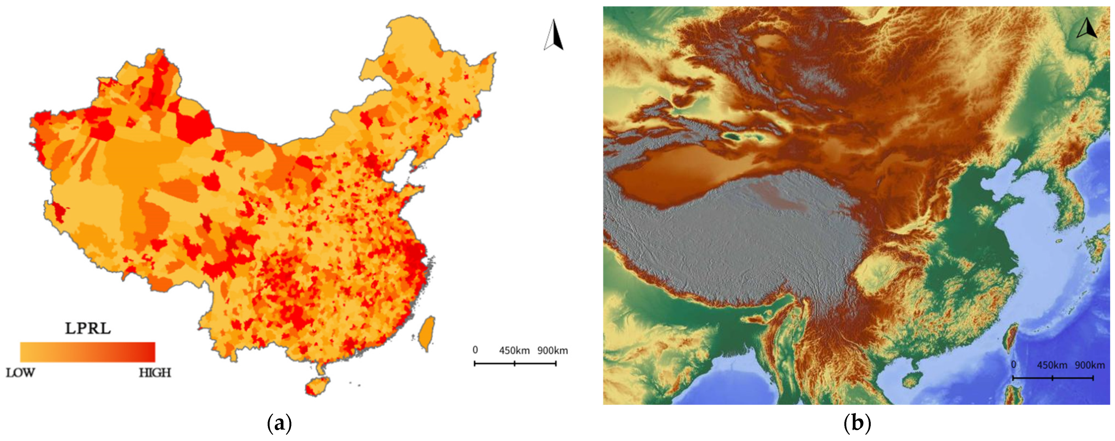
4.1. LPRLA Model Results and LPRL Distribution

Using the combined weighting method, we established the LPRL assessment model and computed the LPRL index for each region. Based on this model, we generated a distribution map illustrating LPRL across different regions. The results are presented in Figure 4 below.

Considering that our various evaluation indicators are based on regional distribution, the varying sizes of regions on the map result from regional delineations. Additionally, we integrated the topography map of China to analyze the distribution of LPRL indices across different regions.

Considering the geographical distribution shown by the light pollution risk level assessment model and the LPRL distribution map, we can draw the following conclusions:

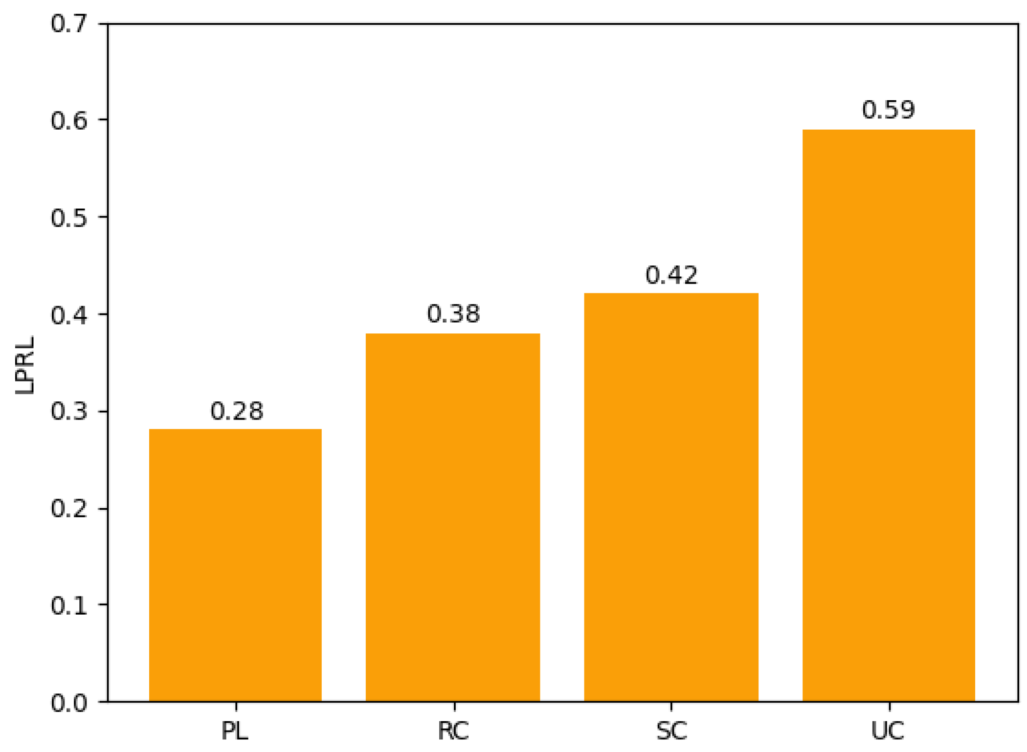
• Each weighting indicator has a similar explanatory effect on the light pollution risk level, ranging from 0.1 to 0.2. This consistency indicates that the selected indicators are reasonably persuasive, and the model is rational.
• The regional development level has the most significant explanatory effect on the light pollution risk level. In this study, we measured regional development using two indicators, POP and GRP, with corresponding weights of 0.1746 and 0.1699, respectively. These indicators rank first and third, respectively, in terms of weight proportion, indicating a substantial influence on the regional development level index. In regions with large populations, high population density results in more significant negative impacts on a greater number of people, even with the same level of light pollution. Moreover, economically developed regions with high housing density have a high demand for electricity. Population concentration often correlates with higher economic levels, GDP, and per capita disposable income. In such areas, there are multiple consumption options and a relatively rich nightlife, leading to the use of all-day lighting for road illumination to ensure safety and convenience. Consequently, light pollution in these areas is more severe, corresponding to a higher risk level.
• Geographically, coastal and mountainous regions tend to have higher LPRL. Coastal areas are economically developed, with flat terrain and dense populations, resulting in significant harm from light pollution. Mountainous areas often have fragile ecosystems and serve as wildlife reserves, where light pollution may have more adverse effects on animals. Therefore, light pollution poses more severe threats to mountainous areas, which face higher levels of light pollution risk.

4.2. Analysis of Regional Differences in LPRL

Based on the light pollution risk level assessment indicators for each city, we clustered all prefecture-level cities nationwide into four categories, labeled PL, RC, SC, and UC. We used the Gaussian mixture model (GMM) algorithm for unsupervised learning to reveal the inherent structures and similarities among cities. The partial results of the city classification are as follows (

Table 4. The partial results of the city classification.

Cluster Categories	City
UC	Shanghai, Beijing, Chengdu, Guangzhou, Wuhan, Chongqing, etc.
SC	Tianjin, Hefei, Jinan, Qingdao, Taiyuan, Nanjing, Shijiazhuang, Zhengzhou, Dalian, Xi’an, etc.
RC	Changchun, Nanning, Guilin, Nanchang, Hangzhou, Haikou, Changsha, Fuzhou, Guiyang, Shenyang, etc.
PL	Kunming, Hohhot, Yinchuan, Urumqi, Lanzhou, Lhasa, Xining, Harbin, etc.

):

Based on the clustering results and the LPRL model, we calculated the average LPRL scores for the PL, RC, SC, and UC regions. The results are as follows (Figure 5):

We can observe the relationship between LPRL and regional clusters: the closer to the city center, the higher the light pollution risk level. Regional classification is significantly correlated with LPRL. For example, areas in top-tier cities like Beijing and Shanghai belong to the UC category, with their LPRL exceeding 0.5. This indicates that LPRL varies significantly across different regions. The further away from the city center, the lower the LPRL, as is also reflected in the results of the LPRLA model.The specific analysis is as follows (

Table 5. Characteristics of the risk level of light pollution in four types of areas.

Impact Metrics	Regional Classification
	PL	RC	SC	UC
LPRL	Relatively Low	Moderate	Slightly Higher	Relatively High
BDS	Relatively remote area with very little daylight and far from big cities.	Near cities or towns, sky light is still present. Other artificial light sources (areas subject to airports, highways) are small.	Closer to a nearby city or town, the sky light level is medium to high.	With a concentration of high-rise buildings, billboards and other artificial light sources, the downtown business district has a very high level of sky light.
CNLI	Artificial management and regulations are strict, and nature conservation is implemented.	Streetlights, outdoor security lights and commercial lighting exist in small towns.	Extensive use of outdoor lighting for commercial and residential purposes.	Street lighting, building façades, and commercial lighting applications are very wide and long-lasting.
LUD	Protected areas, mountainous terrain, relatively low population density, little economic development, and low demand for human artificial light.	The population density is low, and the economy is relatively underdeveloped.	Located near or within a large metropolitan area, hence high population density and high demand and level of artificial light.	It is usually located in the center of a large city, densely populated, with a very developed economy and high levels of artificial lighting.
AASD	Longer natural light hours and shorter artificial light hours resulted in lower LPRL levels in both cases.
WHA	There is a high potential for light pollution of animals in the reserve, but the site is open.	Located near wildlife habitat and may have a negative impact on local wildlife.	May be located near or in wildlife habitat, risk exists.	Wildlife habitat is not generally present.

):

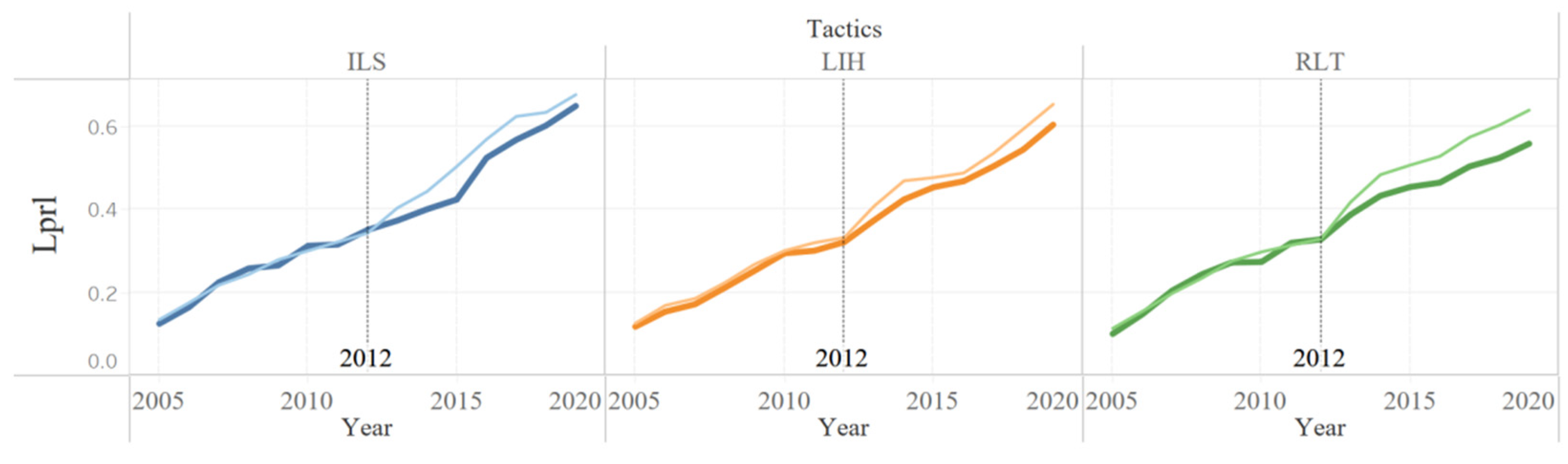
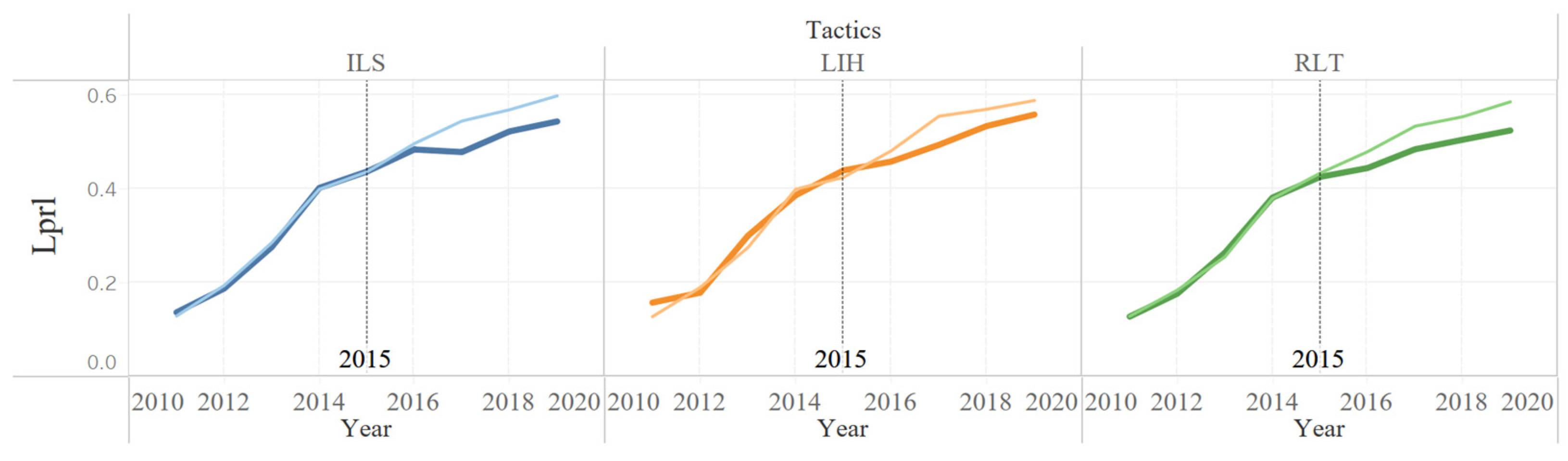
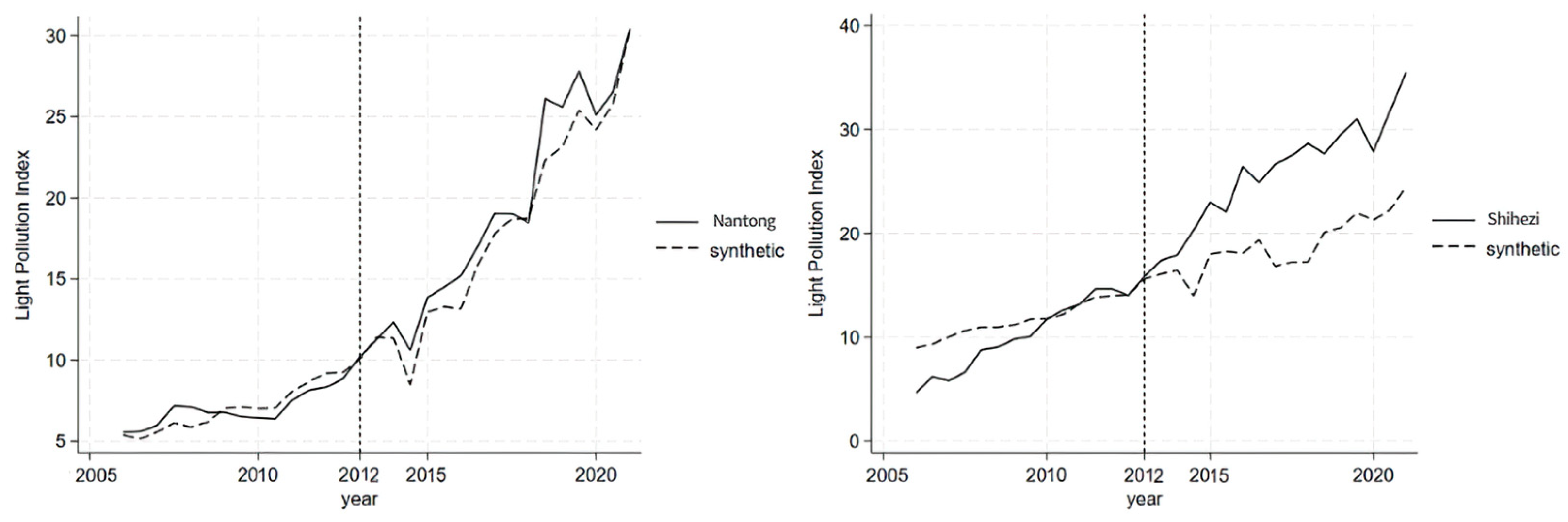
4.3. Three Intervention Strategies

Long-term exposure to white light pollution can cause varying degrees of damage to the retina and iris, leading to a rapid decline in vision. Artificial daylight can also harm birds and insects; intense light may disrupt the normal nocturnal reproductive processes of insects. To address the multiple harms of light pollution, we need to take measures to mitigate this new urban pollution. We propose five policies: reducing lighting duration, improving light sources, upgrading lighting hardware, implementing greening projects, and enhancing community education on light pollution. We hypothesize that each policy has an equal impact on the corresponding indicators. Thus, the higher the correlation between the indicators and LPRL, the more effective the corresponding strategy implementation.

We will perform a correlation analysis between the aforementioned indicators and the LPRL scores from the LPRLA model using the Pearson correlation coefficient. The Pearson correlation coefficient for the sample is represented by ##, and the calculation formula is as follows:

$$r\left(X,Y\right)=\frac{\mathrm{C}\mathrm{o}\mathrm{v}\left(X,Y\right)}{\sqrt{\mathrm{V}\mathrm{a}\mathrm{r}\left[X\right]\mathrm{V}\mathrm{a}\mathrm{r}\left[Y\right]}}$$

(52)

The results are shown in

Table 6. Correlation analysis.

Intervention Strategies	Reduce Light Time (RLT)	Improve Light Sources (ILS)	Improved Lighting Hardware (LIH)	Implementation of Greening Projects (IGP)	Implement Community Education (ICE)
Correlation Coefficient	0.800 **	0.742 **	0.890 **	0.147	0.093

Note: **: p < 0.01.

below.

The correlation coefficient results show that the policies of improving lighting hardware (LIH), reducing lighting time (RLT), and improving light sources (ILS) have the most significant correlation with reducing LPRL. The direct and potential impacts of selecting these strategies on light pollution risk are as follows:

Improving Lighting Hardware (LIH): The use of shielding devices can effectively prevent light from scattering upward, thereby reducing skyglow. Choosing appropriate lighting angles can not only reduce light pollution but lower energy consumption and costs. We advocate for the use of high-efficiency lighting technologies, such as LED lighting, and actively promote new energy-saving light sources. Outdoor lighting fixtures should adhere to dark sky protection standards, such as cutoff luminaires, to ensure minimal light emission.

Reducing Lighting Time (RLT): In urban and peri-urban areas, we recommend implementing nighttime lighting restrictions within communities, turning off non-essential outdoor lights during specific evening hours to reduce energy consumption and costs. Simultaneously, we encourage communities to develop outdoor lighting usage norms and promote the adoption of technologies such as shielding and directional lighting. In rural areas, strict control measures should be implemented to protect the nocturnal environment and minimize the negative impacts of light pollution on wildlife and human health.

Improving Light Sources (ILS): Light sources that are less likely to cause light pollution should be chosen to minimize harm to organisms. Lighting designs should incorporate directional lighting to ensure precise illumination of target areas, reducing light reflection and excessive lighting coverage. We recommend the use of enclosed fixed light sources to promote the application of directional lighting. Additionally, lowering the standard values of lighting intensity is suggested to reduce skyglow and light intrusion issues.

Potential Impacts: (1) The aforementioned three strategies can help reduce light pollution and its associated negative impacts on wildlife, human health, and energy usage. Technological improvements in lighting sources and hardware can promote the development of related products and innovations, injecting new impetus into relevant enterprises and industries. Moreover, the potential impacts of these actions could be significant, as they affect the control of lighting duration, intensity, and coverage. (2) With the mobilization of substantial resources and political will, managers and entrepreneurs can establish a regulatory framework to promote environmentally responsible lighting practices and reduce light pollution. The simultaneous implementation of these three strategies would yield more robust and efficient results compared to implementing just one strategy, thereby facilitating comprehensive light pollution control.

4.4. Analysis of the Three Strategies

We have plotted the time trend of LPRL indices for Changchun and Xi’an against the LPRL indices of the synthetic control group. Please refer to Figure 6 and Figure 7 below.

It can be observed that before the implementation of control policies, the LPRL indices of Changchun and Xi’an (dark lines) were very close to those of the synthetic control group (light lines). However, after the implementation of control policies, the LPRL in the policy implementation areas (Changchun and Xi’an) showed a significant decrease compared to the control group, indicating a noticeable reduction trend in light pollution. This suggests that the impact of light pollution control policies on these two regions is significant.

Given that light pollution arises from multiple sources, reducing its risks is challenging and necessitates coordinated efforts from various stakeholders, including government agencies, lighting design firms, luminaire manufacturers, and the public. Collaboration is essential for improving urban lighting environments and mitigating light pollution. Furthermore, due to the diverse sources of pollution, it is necessary to analyze specific issues related to each cause when formulating and implementing policies, adopting targeted strategies to address them accordingly.

It is through the continuous efforts of society and individuals that we can effectively reduce the level of light pollution risk.

Building upon this analysis, we further examine the impact of the ILS, LIH, and RLT policies on the LPRL indices of Xi’an and Changchun, as shown in Figure 8 and Figure 9.

Prior to the implementation of the three policies, the light pollution risk levels (LPRLs) in Changchun and Xi’an (represented by the dark line) were very similar to those in the synthetic control areas (represented by the light line). Using the data from this figure, we calculated the effects of three strategies—improving lighting hardware (ILH), reducing lighting time (RLT), and improving light sources (ILS)—on LPRL. The corresponding equations are shown below.

$${\alpha }_y=\frac{y_1^{*}-y_1}{y_1}\times 100\mathrm{\%}$$

(53)

The results indicated that among the strategies implemented in Changchun—reducing lighting time (RLT) at 4.84%, improving light sources (ILS) at 4.48%, and improving lighting hardware (ILH) at 3.74%—the RLT strategy was the most effective, reducing the light pollution risk level by 4.84%. In Xi’an, the RLT strategy reduced the risk level of light pollution by 6.10%, compared to ILS at 4.46% and ILH at 3.59%. Thus, RLT was also the most effective strategy in Xi’an.

Reducing lighting time is the most effective strategy for mitigating light pollution in both Changchun and Xi’an. Unlike technical improvements such as enhancing light sources and upgrading lighting hardware, reducing lighting time involves a straightforward change from something to nothing. This approach primarily depends on the control and scheduling by local managers, ensuring high consistency in implementation and minimal operational difficulties. Obviously, controlling artificial lighting can minimize light pollution so as to reduce the harm of light pollution to the local area from the source. Therefore, he is the most direct and effective way to reduce the risk level of light pollution.

In contrast, the strategies of improving light sources and upgrading lighting hardware require significant technology development and prerequisites, such as hardware production, assembly, and replacement. These factors contribute to a high strategic lag, making these approaches less effective compared to reducing lighting time.

4.5. Model Robustness Test

We employed the placebo test method, similar to the falsification test, to evaluate the synthetic control model [56]. The basic idea is as follows: Select a city that did not implement any light pollution control policies during the sample period and conduct a similar analysis. If a significant discrepancy is found between the actual light pollution index of this city and the synthetic light pollution index, and if the synthetic effect mirrors that of the original treatment group, it indicates that the synthetic control method does not provide strong evidence of a significant impact of light pollution control policies on the light pollution index of the original treatment group. Otherwise, it suggests that the results obtained from this method are robust.

In this approach, we select two cities: Nanjing, which holds the highest weight in the synthetic Changchun model, indicating that its light pollution index characteristics are the most similar to those of Changchun and Shihezi, which holds zero weight in the synthetic Changchun model, indicating a significant difference in light pollution index characteristics from Changchun. These two cities serve as extreme cases to examine the actual light pollution index before and after the implementation of light pollution control policies compared to the synthetic light pollution index, as shown in Figure 10 and Figure 11.

Figure 10 presents the results of the placebo test conducted on Nanjing and Shihezi. The results show that the actual light pollution index of Nanjing did not follow the same trend as Changchun’s after 2012. The actual light pollution index of Nanjing fluctuated along the trend of the synthetic light pollution index, while the synthetic light pollution index of Shihezi was lower than the actual light pollution index after 2012, showing an opposite trend to that of Changchun. This indicates that the synthetic control method effectively captured the trend of light pollution indices in both cities. Furthermore, the actual light pollution indices of both cities around 2012 did not decrease below the synthetic level. This provides evidence that the policy implemented after 2012 is a significant factor contributing to the decreased growth rate of the light pollution index in Changchun.

Similarly, we examine the robustness of the synthetic control method for Xi’an. We select two cities: Jinan, which holds the highest weight in the synthetic Xi’an model, and Wenzhou, which holds zero weight in the synthetic Xi’an model. Figure 11 shows the results of the placebo test conducted on Jinan and Wenzhou. The results indicate that the policy implemented after 2015 is a significant factor contributing to the decreased growth rate of the light pollution index in Xi’an.

Based on the above tests, our policy effect evaluation model—which is based on the synthetic control method—can be demonstrated to be rational, reliable, and robust.

5. Discussion

This study establishes an assessment model of light pollution risk levels based on the combination weighting method, aiming to measure and evaluate urban light pollution risk levels. By selecting six indicators covering various aspects such as social development level, environmental factors, geographical features, and climatic conditions (BDS, CNLI, GRP, POP, AASD, WHA), we construct a scientifically rigorous, systematic, quantifiable, operational, and universally applicable indicator system for assessing urban light pollution risk levels. This model can be applied to various types of areas, including urban, suburban, rural, and protected lands.

The allocation of indicator weights is crucial for establishing the evaluation model. Thus, we have chosen a combination weighting method that integrates both subjective and objective approaches to ensure an objective, fair, and reasonable evaluation of the assessed objects based on relevant information. Subjective weighting methods, such as AHP (validated for consistency in this study), have been extensively studied and are relatively mature. These methods determine attribute weights based on the subjective importance assigned by decision-makers or experts. Objective weighting methods, on the other hand, rely on strong mathematical theoretical foundations and do not involve subjective judgments. Examples include IWM, EWM, CV, CRITIC, and PCA. However, relying solely on subjective or objective methods to determine index weights is considered impractical. Integrating these subjective and objective weighting methods into a combination weighting method, such as the combination of AHP, IWM, EWM, CV, CRITIC, and PCA, represents a suitable approach to calculating reasonable weights for each indicator.

Utilizing the aforementioned methodologies, we derived the LPRL index for each region and generated a national LPRL spatial distribution map. When juxtaposed with China’s topographical map, we observed that coastal and mountainous regions typically exhibit higher LPRLs. Additionally, a correlation between proximity to urban centers and elevated light pollution risk levels exists, underscoring the importance of regional classification in LPRL assessment.

Expanding upon the assessment model of light pollution risk levels, we present pertinent intervention policies and conduct correlation analyses. We select three policies demonstrating superior impact and proceed to evaluate their efficacy through a light pollution risk intervention policy test, employing the Gaussian clustering method and synthetic control method. Identifying untreated points akin to the policy implementation points poses a formidable challenge in the testing process. Given diverse factors such as geography, development level, and urban infrastructure, discerning whether discrepancies between two areas solely stem from policy implementation remains arduous. To enhance the precision and scientific rigor of policy effect assessment, we initially employ clustering to identify areas akin to the policy implementation points, subsequently amalgamating other cities from this cluster to formulate a synthetic control group. This approach minimizes disparities in outcomes between the implementation and control groups. Ultimately, our findings reveal that the intervention policies markedly mitigate light pollution risk levels, with light time reduction emerging as the most efficacious policy.

From a theoretical standpoint, this study introduces a novel research perspective into the assessment of light pollution risks, shifting the focus from individual factors such as geography, environment, and production level towards a comprehensive evaluation. This paradigm enhances the evaluation system for light pollution risk levels. In terms of practical implications, the establishment of a referenceable, quantifiable, and universally applicable model for assessing light pollution risk levels offers scientific support and a theoretical foundation for governments to formulate control policies. This facilitates more effective policy-making tailored to diverse regions. Furthermore, the proposed policies and their empirical testing in this study offer practical solutions for policymakers, reducing uncertainties in real-world implementations and ultimately benefiting society at large.

Despite the rigorous and comprehensive nature of this study, there are still areas which need improvement. Firstly, our data are derived from all prefecture-level cities in China. In the next step, we can refine the data to smaller areas, such as counties or even townships, to achieve more precise assessments and predictions, thereby providing more effective research outcomes for local governments. Secondly, due to data acquisition limitations, the most recent data used in our study are only up to 2022. Furthermore, some comparative analyses could only be performed up to 2020 due to the lack of data from many cities, making it difficult to reflect the most current situation. To address this, we will continuously collect the latest data and update our research and conclusions to keep pace with the times. Additionally, more cities are expected to implement light pollution control policies in the future. Future research can examine the effects of these policy implementations more comprehensively, providing more reasonable and universal conclusions and recommendations.

6. Conclusions

Light pollution exerts extensive and profound negative impacts on human society, requesting urgent governance measures. However, interventions should be executed for specific regions, requiring policies adapted to local conditions. Hence, it is imperative to conduct assessments of light pollution risk levels in different regions, evaluate the hazards using multiple indicators, and formulate solutions based on the assessment results. Our study proposes a relative comprehensive assessment of light pollution risk levels and has implemented related policy formulation and effectiveness testing. The research findings indicate that coastal and mountainous areas face higher risks of light pollution, and implementing control policies proves highly effective, with reducing the duration of artificial lighting emerging as the most significant policy measure. This study provides scientific theoretical support and rigorous policy testing for policymakers involved in light pollution governance, holding significant importance and involving significant efforts.

References

1. Guarnieri, M. An Historical Survey on Light Technologies. IEEE Access 2018, 6, 25881–25897. [Google Scholar] [CrossRef]
2. Fouquet, R.; Pearson, P.J.G. Seven Centuries of Energy Services: The Price and Use of Light in the United Kingdom (1300–2000). Energy J. 2006, 27, 139–177. [Google Scholar] [CrossRef]
3. Kyba, C.C.M.; Kuester, T.; Sánchez de Miguel, A.; Baugh, K.; Jechow, A.; Hölker, F.; Bennie, J.; Elvidge, C.D.; Gaston, K.J.; Guanter, L. Artificially lit surface of Earth at night increasing in radiance and extent. Sci. Adv. 2017, 3, e1701528. [Google Scholar] [CrossRef] [PubMed]
4. Lu, Y. The current status and developing trends of Industry 4.0: A Review. Inf. Syst. Front. 2021, 1–20. [Google Scholar] [CrossRef]
5. Schulte-Römer, N. Innovating in Public. The Introduction of LED Lighting in Berlin and Lyon. Ph.D. Thesis, Technical University Berlin, Berlin, Germany, 2015; pp. 321–324. [Google Scholar] [CrossRef]
6. Schulte-Römer, N. Sensory governance: Managing the public sense of light and water. In Sensing Collectives—Aesthetic and Political Practices Intertwined; Voß, J.-P., Rigamonti, N., Suarez, M., Watson, J., Eds.; Transkript: Bielefeld, Germany, 2024; forthcoming. [Google Scholar]
7. Riegel, K.W. Light pollution: Outdoor lighting is a growing threat to astronomy. Science 1973, 179, 1285–1291. [Google Scholar] [CrossRef] [PubMed]
8. Hamacher, D.W.; De Napoli, K.; Mott, B. Whitening the sky: Light pollution as a form of cultural genocide. arXiv 2020, arXiv:2001.11527. [Google Scholar]
9. Svechkina, A.; Portnov, B.A.; Trop, T. The impact of artificial light at night on human and ecosystem health: A systematic literature review. Landsc. Ecol. 2020, 35, 1725–1742. [Google Scholar] [CrossRef]
10. Hatori, M.; Gronfier, C.; Van Gelder, R.N.; Bernstein, P.S.; Carreras, J.; Panda, S.; Marks, F.; Sliney, D.; Hunt, C.E.; Hirota, T.; et al. Global rise of potential health hazards caused by blue light-induced circadian disruption in modern aging societies. NPJ Aging Mech. Dis. 2017, 3, 9. [Google Scholar] [CrossRef] [PubMed]
11. Falchi, F.; Cinzano, P.; Elvidge, C.D.; Keith, D.M.; Haim, A. Limiting the impact of light pollution on human health, environment and stellar visibility. J. Environ. Manag. 2011, 92, 2714–2722. [Google Scholar] [CrossRef]
12. Kuijper, D.P.J.; Schut, J.; van Dullemen, D.; Toorman, H.; Goossens, N.; Ouwehand, J.; Limpens, H. Experimental evidence of light disturbance along the commuting routes of pond bats (Myotis dasycneme). Lutra 2008, 51, 37. [Google Scholar]
13. Brüning, A.; Hölker, F.; Franke, S.; Preuer, T.; Kloas, W. Spotlight on fish: Light pollution affects circadian rhythms of European perch but does not cause stress. Sci. Total Environ. 2015, 511, 516–522. [Google Scholar] [CrossRef] [PubMed]
14. van Geffen, K.G.; van Eck, E.; de Boer, R.A.; van Grunsven, R.H.; Salis, L.; Berendse, F.; Veenendaal, E.M. Artificial light at night inhibits mating in a Geometrid moth. Insect Conserv. Divers. 2015, 8, 282–287. [Google Scholar] [CrossRef]
15. Bennie, J.; Davies, T.W.; Cruse, D.; Gaston, K.J. Ecological effects of artificial light at night on wild plants. J. Ecol. 2016, 104, 611–620. [Google Scholar] [CrossRef]
16. Irwin, A. The dark side of light: How artificial lighting is harming the natural world. Nature 2018, 553, 268–270. [Google Scholar] [CrossRef] [PubMed]
17. Meier, J.; Hasenöhrl, U.; Krause, K.; Pottharst, M. (Eds.) Urban Lighting, Light Pollution and Society; Routledge: New York, NY, USA, 2015. [Google Scholar]
18. MacGregor, C.J.; Pocock, M.J.O.; Fox, R.; Evans, D.M. Pollination by nocturnal L epidoptera, and the effects of light pollution: A review. Ecol. Entomol. 2015, 40, 187–198. [Google Scholar] [CrossRef] [PubMed]
19. Longcore, T.; Rich, C. Ecological light pollution. Front. Ecol. Environ. 2004, 2, 191–198. [Google Scholar] [CrossRef]
20. Hölker, F.; Moss, T.; Griefahn, B.; Kloas, W.; Voigt, C.C.; Henckel, D.; Hänel, A.; Kappeler, P.M.; Völker, S.; Schwope, A.; et al. The dark side of light: A transdisciplinary research agenda for light pollution policy. Ecol. Soc. 2010, 15, 13. [Google Scholar] [CrossRef]
21. Gaston, K.J.; Bennie, J.; Davies, T.W.; Hopkins, J. The ecological impacts of nighttime light pollution: A mechanistic appraisal. Biol. Rev. 2013, 88, 912–927. [Google Scholar] [CrossRef] [PubMed]
22. Agarwal, A.; Xue, L. Model-based clustering of nonparametric weighted networks with application to water pollution analysis. Technometrics 2020, 62, 161–172. [Google Scholar] [CrossRef]
23. Davies, T.W.; Bennie, J.; Inger, R.; De Ibarra, N.H.; Gaston, K.J. Artificial light pollution: Are shifting spectral signatures changing the balance of species interactions? Glob. Chang. Biol. 2013, 19, 1417–1423. [Google Scholar] [CrossRef]
24. Kolláth, Z. Measuring and modelling light pollution at the Zselic Starry Sky Park. J. Phys. Conf. Ser. 2010, 218, 012001. [Google Scholar] [CrossRef]
25. Cinzano, P.; Falchi, F. The propagation of light pollution in the atmosphere. Mon. Not. R. Astron. Soc. 2012, 427, 3337–3357. [Google Scholar] [CrossRef]
26. Pun, C.S.J.; So, C.W. Night-sky brightness monitoring in Hong Kong: A city-wide light pollution assessment. Environ. Monit. Assess. 2012, 184, 2537–2557. [Google Scholar] [CrossRef]
27. Liu, M.; Ma, J.; Su, X.; Zhang, B. The effects of dynamic interference light on human vision, psychology, and emotion. Ergonomics 2009, 15, 21–24. [Google Scholar] [CrossRef]
28. Jieqiao, S.; Lixiong, W.; Mingyu, Z.; Aiying, W.; Juan, Y. Study on Light Environment Partition Control Index Based on Light Trespass Control of Urban Nightscape. China Illum. Eng. J. 2015, 26, 1–6+13. [Google Scholar]
29. Su, X.; Hao, Z. The Research on Lighting Trespass from Roadway Lighting. China Illum. Eng. J. 2012, 23, 46–50+65. [Google Scholar] [CrossRef]
30. Feng, K.; Hao, L.; Zeng, K. Discussion on Evolution Characteristics of Urban Lighting Pollution: Taking Research on VIIRS Images. China Illum. Eng. J. 2022, 33, 1–10. [Google Scholar]
31. Lu, W.; Zhang, X.; Zhan, X. Movie box office prediction based on IFOA-GRNN. Discret. Dyn. Nat. Soc. 2022, 2022, 3690077. [Google Scholar] [CrossRef]
32. Li, M.; Wang, T.; Lu, W.; Wang, M. Optimizing the systematic characteristics of online learning systems to enhance the continuance intention of Chinese college students. Sustainability 2022, 14, 11774. [Google Scholar] [CrossRef]
33. Lu, W.; Xing, R. Research on movie box office prediction model with conjoint analysis. Int. J. Inf. Syst. Supply Chain Manag. (IJISSCM) 2019, 12, 72–84. [Google Scholar] [CrossRef]
34. Lu, W.; Deng, P.; Shen, Z. Research on user stickiness of mobile games. In Proceedings of the 2021 International Conference on Culture-Oriented Science & Technology (ICCST), Beijing, China, 18–21 November 2021; IEEE: Piscataway, NJ, USA, 2021; pp. 160–166. [Google Scholar]
35. Dhanalakshmi, M.; Radha, V. Discretized Linear Regression and Multiclass Support Vector Based Air Pollution Forecasting Technique. Int. J. Eng. Trends Technol. 2022, 70, 315–323. [Google Scholar]
36. Lu, Y.; Ning, X. A vision of 6G–5G’s successor. J. Manag. Anal. 2020, 7, 301–320. [Google Scholar] [CrossRef]
37. Liu, Z.; Mostafavi, A. Collision of environmental injustice and sea level rise: Assessment of risk inequality in flood-induced pollutant dispersion from toxic sites in Texas. arXiv 2023, arXiv:2301.00312. [Google Scholar]
38. Messier, K.P.; Katzfuss, M. Scalable penalized spatiotemporal land-use regression for ground-level nitrogen dioxide. Ann. Appl. Stat. 2021, 15, 688–710. [Google Scholar] [CrossRef] [PubMed]
39. Zhou, Y.; Wei, F. Application of Combinatorial Empowerment Method in Enterprise Performance Evaluation. Ind. Eng. Manag. 2007, 12, 51–54. [Google Scholar]
40. Cao, M.; Xu, T.; Yin, D. Understanding light pollution: Recent advances on its health threats and regulations. J. Environ. Sci. 2023, 127, 589–602. [Google Scholar] [CrossRef] [PubMed]
41. Lima, R.C.; Pinto da Cunha, J.; Peixinho, N. Light pollution: Assessment of sky glow on two dark sky regions of Portugal. J. Toxicol. Environ. Health Part A 2016, 79, 307–319. [Google Scholar] [CrossRef]
42. Kernbach, M.E.; Hall, R.J.; Burkett-Cadena, N.D.; Unnasch, T.R.; Martin, L.B. Dim light at night: Physiological effects and ecological consequences for infectious disease. Integr. Comp. Biol. 2018, 58, 995–1007. [Google Scholar] [CrossRef] [PubMed]
43. Vaz, S.; Manes, S.; Gama-Maia, D.; Silveira, L.; Mattos, G.; Paiva, P.C.; Figueiredo, M.; Lorini, M.L. Light pollution is the fastest growing potential threat to firefly conservation in the Atlantic Forest hotspot. Insect Conserv. Divers. 2021, 14, 211–224. [Google Scholar] [CrossRef]
44. Xiang, W.; Tan, M. Changes in Light Pollution and the Causing Factors in China’s Protected Areas, 1992–2012. Remote Sens. 2017, 9, 1026. [Google Scholar] [CrossRef]
45. Ngarambe, J.; Kim, G. Sustainable Lighting Policies: The Contribution of Advertisement and Decorative Lighting to Local Light Pollution in Seoul, South Korea. Sustainability 2018, 10, 1007. [Google Scholar] [CrossRef]
46. Gili, F.; Fassone, C.; Rolando, A.; Bertolino, S. In the Spotlight: Bat Activity Shifts in Response to Intense Lighting of a Large Railway Construction Site. Sustainability 2024, 16, 2337. [Google Scholar] [CrossRef]
47. Li, J.; Xu, Y.; Cui, W.; Ji, M.; Su, B.; Wu, Y.; Wang, J. Investigation of Nighttime Light Pollution in Nanjing, China by Mapping Illuminance from Field Observations and Luojia 1-01 Imagery. Sustainability 2020, 12, 681. [Google Scholar] [CrossRef]
48. Zielińska-Dabkowska, K.M.; Xavia, K.; Bobkowska, K. Assessment of Citizens’ Actions against Light Pollution with Guidelines for Future Initiatives. Sustainability 2020, 12, 4997. [Google Scholar] [CrossRef]
49. Lu, Y. Implementing blockchain in information systems: A review. Enterp. Inf. Syst. 2022, 16, 2008513. [Google Scholar] [CrossRef]
50. Papalambrou, A.; Doulos, L.T. Identifying, Examining, and Planning Areas Protected from Light Pollution. The Case Study of Planning the First National Dark Sky Park in Greece. Sustainability 2019, 11, 5963. [Google Scholar] [CrossRef]
51. Lu, Y.; Sigov, A.; Ratkin, L.; Ivanov, L.A.; Zuo, M. Quantum Computing and Industrial Information Integration: A Review. J. Ind. Inf. Integr. 2023, 35, 100511. [Google Scholar] [CrossRef]
52. Chen, H.; Xu, Z.; Liu, Y.; Huang, Y.; Yang, F. Urban Flood Risk Assessment Based on Dynamic Population Distribution and Fuzzy Comprehensive Evaluation. Int. J. Environ. Res. Public Health 2022, 19, 16406. [Google Scholar] [CrossRef] [PubMed]
53. Chu, Y. Fire Risk Assessment of Ancient Buildings Based on Combination Weighting Method. Adv. Appl. Math. 2022, 11, 6079–6086. [Google Scholar] [CrossRef]
54. Lu, Y.; Williams, T.L. Modeling analytics in COVID-19: Prediction, prevention, control, and evaluation. J. Manag. Anal. 2021, 8, 424–442. [Google Scholar] [CrossRef]
55. Ye, Z.; Lu, Y. Quantum science: A review and current research trends. J. Manag. Anal. 2022, 9, 383–402. [Google Scholar] [CrossRef]
56. Abadie, A.; Diamond, A.; Hainmueller, J. Synthetic Control Methods for Comparative Case Studies: Estimating the Effect of California’s Tobacco Control Program. J. Am. Stat. Assoc. 2010, 105, 493–505. [Google Scholar] [CrossRef]
Figure 1. Screenshot of some luminous remote sensing images in Shanghai, China.
Sustainability 16 05997 g001
Figure 2. GMM algorithm flowchart.
Sustainability 16 05997 g002
Figure 3. Schematic diagram of the SC model.
Sustainability 16 05997 g003
Figure 4. (a) LPRL of different regions; (b) topographic map of China.
Sustainability 16 05997 g004
Figure 5. LPRL of regional cluster.
Sustainability 16 05997 g005
Figure 6. Synthetic test results for Changchun City.
Sustainability 16 05997 g006
Figure 7. Synthetic test results for Xi’an City.
Sustainability 16 05997 g007
Figure 8. Synthetic test results for three policies in Changchun City.
Sustainability 16 05997 g008
Figure 9. Synthetic test results for three policies in Xi’an City.
Sustainability 16 05997 g009
Figure 10. Synthetic test results for Nantong City and Shihezi City.
Sustainability 16 05997 g010
Figure 11. Synthetic test results for Wenzhou City and Jinan City.
Sustainability 16 05997 g011