Abstract
The use of acrylonitrile butadiene styrene (ABS) in additive manufacturing applications constitutes an elucidating example of a promising match of a sustainable material to a sustainable production process. Lean-and-green datacentric-based techniques may enhance the sustainability of product-making and process-improvement efforts. The mechanical properties—the yield strength and the ultimate compression strength—of 3D-printed ABS product specimens are profiled by considering as many as eleven controlling factors at the process/product design stage. A fractional-factorial trial planner is used to sustainably suppress by three orders of magnitude the experimental needs for materials, machine time, and work hours. A Gibbs sampler and a neutrosophic profiler are employed to treat the complex production process by taking into account potential data uncertainty complications due to multiple distributions and indeterminacy issues due to inconsistencies owing to mechanical testing conditions. The small-data multifactorial screening outcomes appeared to steadily converge to three factors (the layer height, the infill pattern angle, and the outline overlap) with a couple of extra factors (the number of top/bottom layers and the infill density) to supplement the linear modeling effort and provide adequate predictions for maximizing the responses of the two examined mechanical properties. The performance of the optimal 3D-printed ABS specimens exhibited sustainably acceptable discrepancies, which were estimated at 3.5% for the confirmed mean yield strength of 51.70 MPa and at 5.5% for the confirmed mean ultimate compression strength of 53.58 MPa. The verified predictors that were optimally determined from this study were (1) the layer thickness—set at 0.1 mm; (2) the infill angle—set at 0°; (3) the outline overlap—set at 80%; (4) the number of top/bottom layers—set at 5; and (5) the infill density—set at 100%. The multifactorial datacentric approach composed of a fractional-factorial trial planner, a Gibbs sampler, and a neutrosophic profiler may be further tested on more intricate materials and composites while introducing additional product/process characteristics.
1. Introduction
The demand for high-fidelity and low-cost products increased the popularity of an alternative way to build goods, which is known as additive manufacturing [1,2]. To ensure future success, modern production methods need to be sustainable by incorporating globally-instituted initiatives (Sustainable Development Goals # 9 and 12) [3,4]. The emphasis is placed on establishing sustainable production patterns through the adoption of technological innovation. Additive manufacturing, through its unique facility to print a product in separate befitting parts or even in its entirety, has been characterized as a sustainable process across many different industries [5,6,7]. Its seamless alignment to the contemporary Industry 4.0 strategy has created even more opportunities for innovative applications, rendering 3D-printing apt to resolve many production complexity issues under the design freedom to accommodate strict mass customization requirements [8,9,10]. Furthermore, additive manufacturing is distinctive from other methods of production because it unifies the virtual-solid computer-assisted design with the 2D-layer part-design data modeling. The simplification step of the 2D-design segmentation is instrumental in feeding instructions to the 3D-printing equipment so as to create layer-by-layer the manufactured unit. This whole process integrates product design, process design, and product fabrication in an environmentally cautious manner that is evidenced by a perceptible reduction in process waste generation, energy consumption, and gas emissions [11,12,13,14,15]. It is remarkable that additive manufacturing has been proven to be sustainably potent in both demanding areas of manufacturing and construction, in which, in both paradigms, it may be valuable not only to produce in a green engineering fashion but also to be part of broader sustainable applications [16,17,18].
The flexibility that additive manufacturing brings to new product development is unparallel, but it also initiates new challenges that are akin to designing for sustainability while simultaneously improving product functional performance [19,20,21,22]. There are many types of additive manufacturing practices, such as binder printing, inkjet printing, laminate object manufacturing, selective laser sintering, stereolithography, and fused deposition modeling. In this work, we will concentrate on fused deposition modeling (FDM) because of its great versatility in its usage and its inherent decreasing ownership cost of equipment [23,24]. Moreover, eco-design efforts become simpler with this environmentally adaptable method since sustainability improvement projects are susceptible to structured problem solving. A popular cost-effective 3D-printing technique to manufacture plastic parts is fused filament fabrication (FFF). In FFF, 3D-product units are deposited layer-by-layer in stands; they are built by continuous feeding, on a preset layer path, thermoplastic molted threads through an extruding nozzle. Process parameters in plastic material extrusion are influential in aspects with regards to product quality and process greenness [25,26]. Additionally, the material choice that constitutes the extruded filament is of great significance in both stages of material extrusion and in establishing product/process sustainability [27]. One vital aspect of using thermoplastic materials in additive manufacturing is that the extruded waste is recyclable, and this is a sustainable process feature that aids in optimizing terminal product profit [28,29,30,31]. Acrylonitrile butadiene styrene (ABS) is a polymer substance that has appealing properties in FFF applications owing to its high thread formability—a critical property in material extrusion using narrow-diameter nozzles [32,33]. This is attributed to the fact that the ABS polymer, as a feedstock material, is strong, durable, and recyclable under wide conditions of use, wherever chemical and thermal resistance are desirable by design, and, thus, it is considered a sustainable material selection in FFF manufacturing [34]. Nevertheless, depending on the conditions of ABS production and utilization, there might be concerns about material anisotropy on FFF-created parts, and ABS-made part mechanical properties, such as tensile strength and surface roughness, may be influenced by it [35,36,37]. To attain optimal quality performance, the mechanical characteristics of an ABS-made part should be investigated against a score of possible underlying effects in a systematic approach [38]. This is usually accomplished by organizing a study that implements the design of experiments (DOE). The aim of DOE techniques and tools is to screen and optimize a group of controlling factors based on the elicited behavior of one or more mechanical properties [39]. The screening/optimization scheme should be generalizable enough to extend to enduring aspects, such as the improvement of the environmental quality of the FFF product/process, while simultaneously attempting to conduct the perplexing product/process-design optimization phase [40]. Unfortunately, in the case of extruding ABS material in a FFF process using structured experimentation, there is limited published research that involves both themes of multi-variate product quality and sustainability optimization [41]. Mainly, they have been restricted to the examination of only a handful of associated parameters, in spite of the necessity to probe deeper for a broader number of product/process variables. Perhaps it is a practical and economic issue for most research efforts, given the rapidly mounting number of trials that follow the consideration of a larger number of factors.
Enhancing sustainability, lean-and-green principles are integrated into state-of-the-art quality improvement initiatives (Six Sigma) to diagnose, formulate, and resolve difficult operational problems [42,43,44,45]. Lean engineering propounds on the principle of “less of everything”: less waste, less delays, less work, less materials, less time, less emissions, less cost, and so forth [46,47,48,49,50,51]. It is obvious that the lean-and-green engineering goals are closely aligned and so naturally interwoven in the philosophy of additive manufacturing. Carrying out sustainability studies in a structured manner may be fulfilled by adopting the standard toolbox of Green Lean Six Sigma, which primarily consolidates statistical engineering and lean practices [52,53,54]. The statistical engineering part is indispensable to support the scientific validity of the research findings by ascertaining that a quality improvement intervention in a studied process/product has been accomplished [55,56,57,58,59,60]. Introducing sustainable innovation and enhancing environmental quality performance requires new knowledge, which is greatly accelerated by the deployment of DOE methods. By conceiving quick lean-and-green experimental recipes, fractional factorial designs (FFDs) simplify any theoretical approach that seeks to discover a cause-and-effect relationship between controlling factors and process/product characteristics by casting the problem to an empirical model [61]. Since robust products are also sustainable products, orthogonal arrays (OAs)—a particular family of FFDs—may aid in expediting a robust engineering study, thus saving development and production costs as well as reducing product design and manufacturing cycle time [62,63]. OAs also contribute to the sustainability cause in another way by dramatically curtailing the research expenses while shrinking the experimental timetable duration. OA-based experiments demand the use of much smaller amounts of trial materials, reducing personnel work hours, increasing operating equipment availability, and shortening the time to research project completion.
In this work, we attempt to simultaneously screen/optimize a realistic number of controlling factors, a total of 11 variables, for an FFF process using a commercially available ABS material. Under ordinary conditions, such experiments are not feasible—definitely not sustainable—due to the enormous number of accrued trial runs; there cannot be fewer than 211 (=2048) full-factorial trials at a minimum and in the absence of any replication. The purpose is to manage to OA profile the most dominant effects with the goal of maximizing the yield strength and ultimate compression strength for a group of 3D-printed ABS specimens. There are some qualms that may accompany these types of experiments, which involve the testing of mechanical characteristics. Measurement uncertainty is of some concern, and it may be traced to various opportunities that range from equipment calibration and specimen preparation to gripping and alignment to the testing speed and the compression measurement itself. Traditionally, any uncertainty that is raised from such trials, due to the above aspects, is compounded by an unexplainable error. Another aspect might be the effect of the ABS material anisotropy at the small-diameter thread limit, which is imperative to FFF processing—within the same ABS brand and across brands. From a practical standpoint, it is always worth contemplating the measurement precision of such compression strength tests since, during plastic deformation, an ABS specimen experiences some amount of lateral bulging, an occurrence that might introduce some degree of indeterminacy in the mechanical property estimations. Finally, the determination of the operating endpoints for the examined group of controlling factors might be a fuzzy process in itself. This is particularly true if there is a lack of previous knowledge on the factorial relationships among the investigated mechanical properties.
A more general approach would be attempted so as to encompass the inferential approach of classical statistics [55] with fuzzy-oriented systems [64]. Fuzzy sets extend the logic of the two-valued classical objects to partial-truth objects, which are functionally connected by a membership grade between zero and one. From an engineering standpoint, it is desirable to include elements of inconsistency-resilient logic systems (paraconsistent logic) [65]. Hence, the model should be ignorant of the principle of explosion and accept nondualism. The modeling attempt might be benefited if a system of constructive logic (intuitionistic number theory) is also introduced, which could widen the analysis path, oblivious to the law of the excluded middle and the double negation elimination [66,67]. To provide a computability logic to the realizability concerns, neutrosophic statistics have become an attractive means of embracing the above-mentioned logic systems up to the level of intuitionistic fuzzy logic [68,69,70,71,72]. The neutrosophic logic has been shown to be operative in classical inferential methods such as the analysis of variance, correlation, and regression [73,74,75]. Furthermore, this computational convenience has been exploited to resolve complex problems that range from quantifying anisotropy effects in rock mechanical properties to sustainable biomedical-waste management, sustainable car recycling, white-blood-cell segmentation, nanoparticle rating, quality evaluation, and opinion mining in forming perspectives [76,77,78,79,80,81,82,83].
The novelty of this work relies on implementing the versatility of the neutrosophic regression approach to an ‘all-purpose profiler’, which should be capable of being applied to a multi-response OA-sampled dataset. It would be demonstrated by screening/optimizing a group of several controlling factors by maximizing the yield and compression strength properties of 3D-printed ABS specimens. The neutrosophic-based predictions will be compared to randomized algorithm results, which will be obtained by the Gibbs sampler [84,85,86]. Gibbs regression is used in Bayesian inference to sample from a conditional distribution by approximating the marginal distribution of the variables and, hence, to generate an approximate joint distribution when direct sampling from the examined multivariate probability distribution is not guaranteed. Additionally, the neutrosophic-logic/Gibbs sampler FFD dataset regression analysis will be compared to the more classical inference methods of quantile regression for robustness and stepwise regression to detect any prediction discrepancies. The screening/optimization results will be discussed against the confirmation outcomes in order to assess the success of this research endeavor.
The rest of the paper describes a methodology for setting up and executing the orthogonal multifactorial experiments for the maximization of yield strength and ultimate compression strength responses. In addition, basic information on neutrosophic and Gibbs sampler regression analysis is presented, which is computationally facilitated by the respective R software modules. The outcomes of the multifactorial profiling are explained in the Results section. A Discussion section compares the viability of the suggested solutions by comparing the profiling hierarchy status from neutrosophic/Gibbs sampler regression to more mainstream statistical solvers such as stepwise regression analysis and the more robust-oriented quantile regression analysis. A conclusion section summarizes the importance of the findings in this research effort.
2. Materials and Methods
2.1. Experimental Methods
2.1.1. The Experimental Setup
The modeled specimen is a cubic part with a side length of 10 mm [87]. The 3D CAD Design Software Dassault Systemes Solidworks (version 2017) (Dassault Systemes, Velizy-Villacoublay, France) was utilized to design the 3D solid structure. It also permitted establishing the converted coordinates on a 3D using triangles to capture the outer surface tessellation of the modeled unit. The design information was created as a sequence of formed triangles that encapsulated the entire modeled specimen volume; it was stored as a stereolithographic model (STL format) in order to be loaded on the slicer software. The stored information was the coordinates of the assembled triangle vertices and the coordinates of the area normal to the vector that exits the cubic specimen surface. The cubic volume of the specimen was converted to successive 2D horizontal layers via triangular meshing using the slicing software Simplify3D (version 3.3) (Simplify3D, Cincinnati, OH, USA), which is suitable to program additive manufacturing applications; it also aided in facilitating proper adjustments in order to achieve a satisfactory 3D-printing resolution. The 3D-printable unit consists of a stack of individually printed platforms. Each platform is an accumulation of 2D toolpath lines. The required settings for the extruder and the layer details, the infill patterns, the 3D-printing process temperatures, any raft additions, the 3D-printing process speed selections, the fed filament properties, the G-code, and the other process scripts were entered in the Simplify3D input menu (Figure 1). The 3D-printing procedure was translated into a numerical control program (NC files) using G-code, and it was based on a Cartesian 3D axis system.
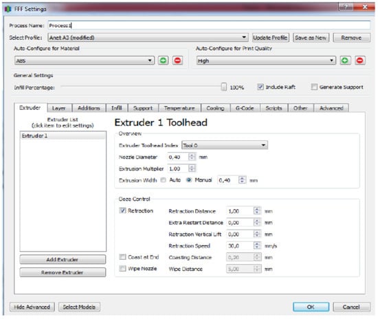
Figure 1.
Entering the vital 3D-printing process parameters in the Simplify3D slicer software.
The 3D-printing machine configuration was assigned build volume dimensions of 150 mm × 150 mm × 150 mm with respect to the X, Y, and Z axes, respectively. The origin offset was set at (0, 0, 0), and the machine type was a Cartesian robot, geared to deal with a rectangular volume. The temperature instruction was “Heated bed” and the selected material type was “ABS”. The scheduled batch program allowed three replications at the preset conditions. The choice “Outside-In” was the preferred outline direction in the “Layer” requirement because it helped to attain better dimensional precision. The dimensional adjustment to compensate for horizontal deviations was set at −0.05 mm.
To conduct the fusion-based filament fabrication task, the industrial-grade thermoplastic polymer, acrylonitrile butadiene styrene (ABS), was investigated. Owing to its unique mechanical properties and its heat resistance capabilities, the ABS polymer is applicable to both interior and exterior usages. The 3D-printed ABS material was treated in a heated bed, which was regulated at a temperature range of 80 °C to 110 °C. The extruder temperature could vary from 220 °C to 260 °C. For the particular set of experiments, it was necessary to attach an enclosure to isolate the 3D-printing area. The blower fan was not turned on during the experiments.
The ABS filament that was chosen for the extrusion experiments was the Neema3DTM ABS EVO Ultimate filament (Neema3D, Petroupolis, Greece). Several features rendered its usage advantageous: (1) its low propensity for cracking; (2) its enhanced warp resistance; (3) its stable behavior in bed and interlayer adhesion; (4) its more manageable handling during production; (5) its low cost; and (6) its additive manufacturability to fabricate larger items. Generally, ABS materials exhibit favorable tendencies in compression and impact tests. This particular ABS material type was processed at a standard bed temperature set at 80 °C. The extruder was a modular 3D printer, Anet 3D, model A3-S (Shenzhen Anet Technology, Longhua, Shenzhen, China). This FFF machine had an available printable volume of 160 mm × 160 mm × 150 mm, a printing resolution in the range of ±0.1 mm to 0.15 mm, and a layer thickness range of 0.1 mm to 0.4 mm. Furthermore, the maximum extruder and hotbed temperatures were specified at 250 °C and 100 °C, respectively. The movement and printing speed ranges were specified at 10 to 300 mm/s and 40 to 120 mm/s, respectively. The nozzle size was 0.4 mm, and the filament diameter was 1.75 mm. The hotbed material was aluminum PCB, and the printer could operate in either online or offline modes. The printer head was heated up to 245 °C, bed leveling was carried out, and the machine was calibrated with a standard cube (side length of 20 mm). The printer was conditioned by a ventilator. The printing chamber was isolated by a paper box to stabilize the internal temperature conditions.
Compression tests—driven to fracture—were carried out on a testing machine Z010 Zwick/Roell (Zwick/Roell, Ulm, Germany), with maximum load capability of 10 kN, preload at 1000 N, sample size (n) at 3, and test speed at 1 mm/min. The testing machine was suitable for compression, tensile, shear, flexure, and cyclic tests, furnishing versatile measurements for metals, plastics, and textile materials. The complete experimental cycle is shown in Figure 2.
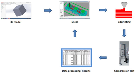
Figure 2.
A schematic portrayal of the key procedural steps to conduct the ABS 3D-printing compression strength trials.
2.1.2. The Selected Controlling Factors, the Mechanical Characteristics, and the Trial Planner
The proposed additive manufacturing model was based on a multi-factorial linear design, seeking to accomplish the profiling of potential active effects [87]. The eleven controlling factors, their experimental settings, and their coded labels that were examined in this work are tabulated in Table 1. The layer thickness affects the 3D-printing quality—physical and mechanical properties—the total 3D-printing time and the production cost. The number of top/bottom layers is crucial in reinforcing either side with solid 100%-infill-density layers at the beginning and end of the cubic structure, at its two opposite sides. The number of outline shells strengthens the 3D-printed structure by providing external casings at a comparable width to match that of the 3D-printer’s nozzle diameter. The two selected operating endpoints were the practical limits to ensure structure rigidity (2 shells) and to permit the designed infill generation (10 shells). After a series of preliminary tests, the selected infill pattern was finalized on the Simplify3D software package by picking the option “Rectangular”. Therefore, the appropriate settings were as follows: (1) the rectilinear [0°] configuration that was examined at the Y-Z level; and (2) the rectilinear [45°, −45°] configuration with alternating layer angle offsets at 45° and −45° across parallel toolpath lines. Both available external patterns in the Simplify3D software package were tested in their rectilinear and concentric forms. The outline overlap was maintained at higher percentages to test the rigidity of the unit when the shell framing and the infill-pattern bordering frames almost coincided. The experiments were run with no solid diaphragm (100% infill density layer) and also with a diaphragm—to further enhance structure rigidity—in every three 3D-printed layers such that they match the configurations of the pre-selected top/bottom layers (rectilinear/concentric patterns). The printing speed is an essential parameter that influences the quality of the infill layout and the production performance of the 3D printing process. The insertion of a raft as a substrate between the part unit and the bed surfaces in order to enhance adhesion was also tested. The extruder temperature is pivotal to polymer filament melting, and it is highly dependent on the material type. Selecting high extruder temperature ranges favors the onset of the stringing effect and the appearance of failing bridging patterns. On the other hand, a low extruder temperature reduces the filament flow capability; it interferes with the proper extruder function by promoting wear and breakdowns while impeding product adhesion and accelerating delamination. The infill density, expressed in percentages, indicates the extent of material coverage in a 3D-printed layer. It is correlated to the part unit rigidity and weight, as well as to the total cost of manufacturing and the total production cycle time.

Table 1.
Controlling factor list for the ABS 3D-printing compression strength experiments.
To effectuate a sustainable experimental plan, the Taguchi-type L12(211) OA was implemented to dramatically condense the number of the necessitated trial runs. The benefit that is derived from this choice is easily demonstratable. A comprehensive full-factorial sampling scheme would dictate as many as 211 (=2048) trials (without counting the multiplicative effect of making provisions for replicated experiments). Planning for a triplicate trial schedule, this would forecast massive research work consisting of 3 × 2048 = 6144 trials. Overall, the sustainable approach that is proposed in this work would reduce the demand for resources, research time, and manhours by a factor of 2048/12 ≈ 171. These are extraordinary gains, which essentially permit, from a practical standpoint, the realization of such a project. In Table 2, the experimental plan is completed in saturated form (maximum trial planner utilization), coded according to the labeled controlling factors from Table 1; the factorial settings are also included in the table. It is seen that eight factors are numerical variables and three are categorical variables. The proposed quality characteristics are the two mechanical properties of the 3D-printed product unit: the yield strength and the ultimate compression strength. Both output responses are measured in MPa.
Table 2.
The L12(112) OA trial planner for the 3D-printer ABS mechanical property experiments.
2.2. Data Analysis
2.2.1. The Neutrosophic Profiler
A linear OA sampler is selected to condense the experimental control combinations to a degree much less than what is dictated by a corresponding full factorial design. The screening design is a predefined matrix that can accommodate an arrangement of numerical and categorical controlling factors. In sustainable datacentric engineering applications, the OA sampler is a blueprint for a planner that organizes a few informative trials. The OA matrix is an n × m array, in which the n rows represent the predefined experimental recipes and the m columns identify the controlling factor adjustments that are necessary to execute the trial runs [61,62,63]. For practical purposes, the OA sampler is assumed to be implemented in saturation mode (maximum utilization of the sampling capacity). Hence, for a selected two-level OA, the relationship between the number of rows and columns is n = m +1. The m controlling factors examined are defined as follows: Xj for 1 ≤ j ≤ m (m ϵ N), and their respective factor settings are denoted as xij for 1 ≤ i ≤ n (n ϵ N) and 1 ≤ j ≤ m. The multi-characteristic response matrix Y = {yicd}, with 1≤ i ≤ n, 1 ≤ c ≤ C (C ϵ N), and 1 ≤ d ≤ D (D ϵ N), is generated by C characteristic responses, Yc; each cth matrix column is replicated D total times. Since there are a total of D trial replications, then, for each experimental recipe, i, the dataset may be converted into a neutrosophic interval dataset [68,69,70,71], where only the lower and higher replicate values are retained in the neutrosophic formalism. In other words, for a given recipe run, i, and a characteristic, c, the replicates {yicd} for 1 ≤ d ≤ D become [yLic, yUic], where yLic = min{yicd} for 1 ≤ d ≤ D, and yUic = max{yicd} for 1 ≤ d ≤ D. In the symbolic neutrosophic theory, indeterminacy is introduced by additively splitting a neutrosophic number into a determinate and an indeterminate part. The indeterminate part may be sampled from a range of [0, 1] proportional to the coefficient value of the yUic-yLic. This is because in Smarandache‘s neutrosophic logic, there are three distinct degrees for (1) truth (t), (2) indeterminacy (i), and falsehood (f). The intriguing feature is that any of the t, i, and f may be standard or non-standard subsets of the non-standard unit interval [−0, 1+], which means that the totaling of the three subsets is great or equal to −0 and less or equal to 3+. After the original replicated multi-response datasets have been transformed in terms of multi-response neutrosophic variables (Table 3), they may be straightforwardly analyzed using the neutrosophic linear regression method of Nagarajan et al. [74]. The neutrosophic profiler also returns interval data from the regression coefficients of the partaking controlling factors. This completes this novel multi-factorial neutrosophic screening process for the examined quality characteristics.
Table 3.
The OA planner and the neutrosophic interval data output vectors.
2.2.2. Screening a Multifactorial OA Design with a Gibbs Sampler
The Gibbs sampler is a computer-intensive statistical method that may be used to enable the screening of factorial effects from data that are collected from linear orthogonal arrays. A great advantage of the method is that it sidetracks the calculation of a joint probability density function by assembling the behavior of the examined random variables indirectly from their individual marginal distributions [84,85,86]. Since linear regression is required to provide the effect contributions through a linear approximation of the factorial coefficients, a Gibbs sequence of the random variables is formed by alternating the generation of conditional probabilities between inputs and outputs in a simple iterative scheme. Considering that the general linear modeling of a number of m quality characteristics, Y, and owing to an n number of controlling factors (defined at two endpoint settings), X, then the coefficients of the regression vector β are simply given by the following:
Y = Xβ + ε with ε ~ N(0, σ2) and β ~ N(μ, σ2) and σ2 ~ Γ−1(α,β)
Therefore, the posterior conditional probabilities, due to the observed data, allow the estimation of the central tendencies and variabilities of the regression coefficients, which can then be iteratively created as follows:
and therefore, the distribution of the coefficients of regression may be approximated as follows:
where σ2|Y, β ~ N(Xβ, σ2) Γ−1(α,β) ~ Γ−1(αn,βn), given that αn = a + n/2 and βn = (Y − Xβ)′ (Y − Xβ)/2, where αn, βn are the shape and rate parameters of the Gamma function prior, respectively.
p(β, σ2|Y) ∝ N(Xβ, σ2) N(μ, τ2) Γ−1(α,β)
β|Y, σ2 ~ N(m, s) with m = (X′X)−1 X′ Y and s = σ2 (X′X)−1
2.3. The Methodological Outline
The proposed methodological approach may be summarized in the following steps:
- (1)
- Determine the basic structural characteristics of the 3D-printed ABS specimens and indicate the mechanical properties that will be monitored—the yield strength and the ultimate compression strength—as well as their direction of improvement.
- (2)
- Select an extensive group of controlling factors that might influence the output quality of the 3D-printed ABS product-unit characteristics.
- (3)
- Determine the operating range for each individual controlling factor from step 2, and define the factorial end-point settings.
- (4)
- Select an orthogonal trial planner that adjusts all factorial settings, from step 3, in a formulation schedule that requires the least number of recipes in the sampling scheme.
- (5)
- Test replication adequacy, data normality, and correlations among the characteristic responses.
- (6)
- Perform factorial screening using neutrosophic regression to determine the leading factorial effects by casting replicated data into interval data.
- (7)
- Implement Gibbs sampling to confirm the leading regressors by computing the posterior conditional distributions in a single dataset that consolidates all replicates.
- (8)
- Determine any factorial prediction discrepancies using more ordinary treatments such as stepwise regression analysis and the robust quantile regression method.
- (9)
- Propose an optimal solution for the linear approximation study.
- (10)
- Confirm whether the predicted recipe from step 9 might be practically sustainable before advancing to more sophisticated experimental strategies, if they are needed.
2.4. The Computational Support
The descriptive statistics for the yield strength and the ultimate compression strength datasets, the normality tests (Kolmogorov–Smirnov and Shapiro–Wilk tests) for the individual replicate OA data, as well as in their combined form, the correlation tests between the two characteristics for each replicate dataset, the linear regression analysis for the two characteristics for each replicate dataset, the linear regression analysis within each characteristic for all replicate two-way combinations, and finally, the multifactorial stepwise regression analysis for the combined datasets of the two characteristics were all computed in the statistical software package IBM SPSS v. 29.
The dedicated computational work was implemented on the statistical freeware platform R (v. 4.3.0) [88]. The basic visual dataset screening of the yield strength and the ultimate compression strength was conducted using boxplots, beanplots, and Q-Q plots from the R packages ‘graphics’ (v. 4.3.0), ‘beanplot’ (v. 1.2), and the module ‘qq_conf_plot()’ of the R package ‘qqconf’ (v. 1.3.1), respectively. The L12(211) OA array was constructed using the module ‘param.design()’ from the R package ‘DOE.base’ (v. 1.2-2). The linear regression analysis of the neutrosophic interval dataset for yield strength was accomplished by the module ‘lm()’ in the R package ‘stats’ (v. 4.3.0). Consequently, the factorial effects from the two neutrosophic interval dataset limits were contrasted using the classical Lenth test (module ‘LenthPlot()’) from the R package ‘BsMD’ (v. 2020.4.30). The module ‘lm()’ was also deployed to furnish the graphical line-fitting between the two mechanical properties for each individual replicate; it also included the 95% confidence interval band. The R package ‘ntsDists’ (v. 2.0.0) was utilized to test some of the neutrosophic distributions that were generated from the neutrosophic linear regression procedure. The linear regression analysis exploiting the Gibbs sampler was performed by the R package ‘lrgs’ (v. 0.5.4) [89]. The module ‘Gibbs.regression()’ was tuned to sample 10,100 times in order to simulate the marginal distributions; the first 100 points were removed from the data processing as they were considered part of the burn-in period. The quantile-regression profiling of yield strength data was verified by the R packages ‘quantreg’ (v. 5.97) and ‘SparseM’ (v. 1.81).
3. Results
3.1. Data Screening for Yield Strength and Ultimate Compression Strength
Conducting the experimental recipes, which are formulated by the L12(211) OA (Table 2), we 3D-printed 12-triplet specimen cubes (side length of 1 cm); specimens are arranged per OA run order in Figure 3 (ref. [87]). The yield strength and the ultimate compression strength triplicate measurements have been tabulated in increasing run order in Table 4—both in MPa units [87]. The basic descriptive statistics for the three replicated runs of the yield strength and the ultimate compression strength are listed in Table 5. Based on the summary statistics, there are three remarks to be made: (1) the yield strength measurement means across the three replications are statistically similar; (2) the ultimate compression strength measurement means across the three replications are also statistically similar; and (3) the margins of error for the yield strength and the ultimate compression strength measurements allow the two intervals to overlap for each individual replicate dataset. It appears that the last remark is statistically significant at a level of α = 0.05 for all three replicated datasets. Hence, knowing one of the two characteristics, it might be simple to guess the behavior of the other. Before commenting further on the predictability between the two characteristics, it is informative to examine the shape statistics as well as the normality status across the replicated datasets and between the two characteristics. From Table 5, the skewness values for all replicates are similar at first glance, indicating data symmetry across all replicates. However, by taking into account their standard error estimations, asymmetry may not be precluded, leaving it indeterminate which sides the long tails point to in their respective data distributions.
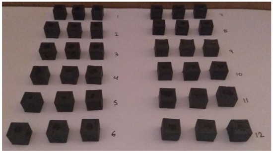
Figure 3.
The 12-run (three-times) replicated (L12(211) OA) 3D-printed ABS cubic specimens.
Table 4.
Yield strength (YS) and ultimate compression strength (UCS) measurements (in MPa) for the L12(211) OA-replicated trials (Table 2).
Table 5.
Descriptive statistics for yield strength (YS) and ultimate compression strength (UCS) replicated trials (IBM SPSS v. 29).
Similarly, kurtosis estimates are indeterminate for all six datasets because their standard errors permit all three typical kinds of tail patterns to be manifested (platykurtic, mesokurtic, or leptokurtic). However, the kurtosis point estimates approximately match both characteristics for each separate replicated dataset. Testing the six collected datasets for normality using the Kolmogorov–Smirnov and Shapiro–Wilk methods (Table 6), we observe that all but the first replicate dataset for the ultimate compression strength appear to agree with a random structure at a level of significance of α = 0.05. Still, this only-exception finding is actually a split decision between the two utilized goodness-of-fit tests, as the p-value of 0.046, which is obtained from the Shapiro–Wilk test, may be construed as a marginal departure from normality.
Table 6.
Replicate dataset (dual) normality tests for yield strength (YS) and ultimate compression strength (UCS) (IBM SPSS v. 29).
On the other hand, in the boxplot screening of the six replicate datasets (Figure 4), the extent of asymmetry in the second and third specimen replications, for both mechanical characteristics (YS and UCS), is more pronounced than that of the ultimate compression strength measurements from the first replication. Incidentally, the behavior of the UCS data from the second specimen replication appear more unbalanced in comparison to the other two replicated datasets. Visually, the boxplot for the second replication dataset of YS depicts a noticeable asymmetry, which is rather not supported by either of the two goodness-of-fit performances of Table 6—p-values of 0.15 and 0.64, respectively.
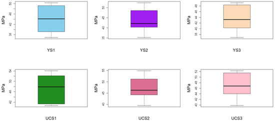
Figure 4.
Boxplot screening for each individual 3D-printed ABS specimen replication: YS-yield strength; UCS-ultimate compression strength.
Those disagreements between graphical and statistical results prompt additional rounds of data screening. Beanplot screenings (Figure 5) of the three replications do not hint at any skewness for either of the two mechanical characteristic datasets that are related to the second replication. Nevertheless, the pair of beanplots that relate to the first replication might suggest a trace of bimodality in the data, a trend that might also be extended to the yield strength response in the third replication of the experiments. Finally, a QQ-plot screening of the three replications is provided in Figure 6. Two remarks may be made: (1) the band expansion around the trend line is substantial, and this may influence the precision of mechanical property predictions; and (2) there is a lopsidedness in the accumulation of the data points around the QQ-plot trend line, which is accentuated as a “half-banded” irregularity in the QQ-plots of the observations of the second replication of the yield strength and the second and third replication observations of the ultimate compression strength.
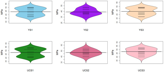
Figure 5.
Beanplot screening for each individual 3D-printed ABS specimen replication: YS-yield strength; UCS-ultimate compression strength.
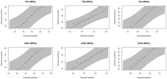
Figure 6.
QQ-plot screening for each individual 3D-printed ABS specimen replication: YS-yield strength; UCS-ultimate compression strength.
3.2. Testing Correlations for Yield Strength and Ultimate Compression Strength Response Data
To decide whether to include both mechanical properties in the multifactorial screening process, a correlation analysis between the yield strength and the ultimate compression strength was attempted for each replicated dataset separately. From Table 7, it is evident that there is a high positive correlation between the two mechanical properties; the correlation coefficient estimates are maintained high in all three independent replications. Furthermore, the range of the coefficients of correlation was narrow, and their values varied between 0.970 and 0.979. The upper and lower bounds for the correlation coefficients, according to their 95% confidence intervals, were as high as 0.994 and no lower than 0.894, respectively. Next, it was enquired how well the prediction results could apply to both characteristics while retaining only one of the two characteristics in the factorial analysis that would follow. For instance, to check the redundancy of the ultimate compression strength response in the screening phase, a regression analysis was carried out between the yield strength and the ultimate compression strength data (Table 8). The standardized linear regression coefficients were sufficiently close to one for all three replications; they ranged from 0.97 to 1.04. However, the second replication dataset produced an intercept value in the unstandardized fittings that was statistically significant at a level of 0.05.
Table 7.
Correlation analysis for yield strength (YS) and ultimate compression strength (UCS) replicated trials—C.I. level: 95.0% (IBM SPSS v. 29).
Table 8.
Regression analysis between yield strength (YS) and ultimate compression strength (UCS) replicated trials (IBM SPSS v. 29).
This behavior was matched to a higher Durbin–Watson test statistic score, which was estimated at a value of 3.12; it might signify a negative autocorrelation in the successive error terms. However, the adjusted coefficients of determination were fairly consistent among the three replications, and they ranged from 0.936 to 0.954.
3.3. Testing Replication Adequacy for Yield Strength and Ultimate Compression Strength Data
A practical way to test replication adequacy for yield strength and ultimate compression strength in saturated OA-generated datasets might be to apply cross-regression between all replicated dataset pairs. In Table 9, the linear regression analysis results are tabulated for the six replication pairings of the two mechanical characteristic responses (IBM SPSS v. 29). The general observation is that all six coefficients of regression are statistically significant at a level of 0.05. No intercept values were statistically significant for the yield strength data. Moreover, the intercept estimations for the two out of the three tested pairs of the ultimate compression strength were not statistically significant (α = 0.05); the intercept estimate for the tested pair of the first and third replications was found to be statistically significant, though. For the yield strength, the slopes ranged from 0.69 to 0.85, which may be viewed as a rather satisfactory outcome, given the complexity and the committed resource limitations of the selected experimental design. Similarly, the ultimate compression strength slopes ranged from 0.75 to 0.80, which may be viewed as adequate.
Table 9.
Linear regression analysis for yield strength (YS) and ultimate compression strength (UCS) replicated trials (IBM SPSS v. 29).
Based on the adjusted coefficients of determination scores for the yield strength, the presence of the dataset that is associated with the second replication tends to lower the adjusted R2 estimation to a marginal value of 0.63; it probably provides additional evidence for amplified variability concerns that are tagged to the second replication. This behavior is also consistent with the linear regression outcomes for the ultimate compression strength data. In this case, the fitting performance, according to the adjusted coefficient of determination estimate, improves to 0.71.
Finally, a graphical representation furnishes additional information about the replication trends between the different pairs. In Figure 7, the fitted line plots are shown for all six combinations of the three replications and for both mechanical characteristics. The main observation is that in all graphs, several points may be found outside the 95% confidence interval band. This manifestation may not explain how additional replications would have improved on this behavior, i.e., to better confine the data points within the confidence interval bounds.
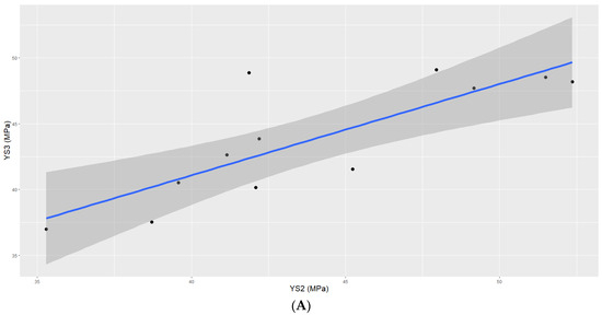
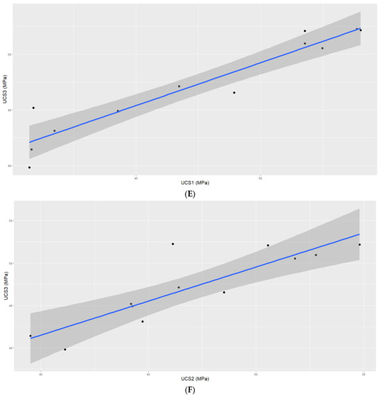
Figure 7.
Line fitting with a 95% confidence interval band for the yield strength (YS) and ultimate compression strength (UCS) measurements of the 3D-printed ABS specimens: (A) YS3 vs. YS2, (B) YS3 vs. YS1, (C) YS2 vs. YS1, (D) UCS2 vs. UCS1, (E) UCS3 vs. UCS1, (F) UCS3 vs. UCS2.
3.4. Neutrosophic Multifactorial Profiling of the Yield Strength Response
The results from the previous sub-sections imply that, in addition to stochastic uncertainty, indeterminacy should probably be included in the progressive analysis of the multi-factorial datacentric model. From the completed correlation analysis, we infer that the design problem may be reducible to a single characteristic. Thus, the yield strength response is selected to solely represent the output signature in the data treatment that ensues. The original replicated dataset of the yield strength (Table 4) is cast in terms of interval data (YSnv), and next it is easily transformed into a single neutrosophic variable (YSInv) in Table 10. The neutrosophic variable has a determinate part and an indeterminate part. In all 12 cases, it holds that the indeterminate part is formed by considering that I ϵ [0, 1].
Table 10.
The replicated yield strength (YS) dataset expressed as a neutrosophic characteristic response (MPa).
The transformed model requires executing the multi-factorial linear regression analysis twice [74]—each for either of the two bounds. However, the problem is now reduced to treating two unreplicated–saturated OA datasets. This development requires first estimating twice the regression coefficients at the two bounds and then deciding on their statistical significance by utilizing a specialized technique that converts the unreplicated–saturated OA design datasets.
In Table 11, the neutrosophic regression coefficients results are listed in both forms as interval data bounds ([Cys,L, Cys,U]) and as a single neutrosophic variable (CIys) for I ϵ [0, 1]. It is quickly noticed that factors C (number of outline shells), E (external pattern), G (diaphragm), and J (extruder temperature) are weak. The rest of them may be considered for further exploration. The controlling factors that seem to lead to the strength hierarchy are as follows: (1) D (infill angle): 3.75 + 0.56I (MPa); (2) F (outline overlap): 2.25 + 0.40I MPa/% (3) I (use of raft): −2.38 + 0.64I MPa; (4) A (layer thickness): −1.70 − 0.56I MPa/mm; (5) B (number of top/bottom layers): 2.11 − 0.72I MPa; and (6) K (infill density): 1.14 + 0.76I MPa/%. Out of the six controlling factors, the opposing influence on improving yield strength performance is identified as smaller layer thickness and the absence of a raft. To supplement the neutrosophic profiler with a statistical comparison of the effects, the Lenth test is employed for practical levels of significance set at α = 0.10, 0.20, and 0.40. From Figure 8, a clearer profile is observed when the significance level is set at α = 0.40. Considering the performances from both neutrosophic regression coefficient bounds, factors D, F, and A are exceeding the margin of error (ME) mark. Factors B and I join the list when restricted to the lower bound estimations. On the other hand, the upper bound estimation may suggest replacing the I to K effect. It is interesting that at levels of significance set at α = 0.10 and 0.20, only the controlling factor D (infill angle) is identified as the predominant strong effect.
Table 11.
Neutrosophic regression coefficient results for the eleven controlling factors against the yield strength (YS).
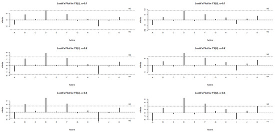
Figure 8.
Lenth plots of the yield strength (YS) at the upper (U) and lower (L) neutrosophic effect limits for ME significance levels set at α = 0.1, 0.2, and 0.4, respectively.
4. Discussion
The results from the previous section necessitate further probing using different tactics, since the application of neutrosophic screening in the FFD-planned dataset is novel. A naïve first move is to assemble all 36 observations in a single dataset and analyze it accordingly. After repeating the application of the two tests of normality and removing the replication identity from the datasets, we estimated the Kolmogorov–Smirnov and Shapiro–Wilk test statistic scores in Table 12. This time, both goodness-of-fit test results agree that the behavior of the ultimate compressive strength dataset may deviate from normality at a level of significance of α = 0.05. There is a split decision on the yield strength dataset, in which the Shapiro–Wilk test outcome may indicate that the normality hypothesis is marginally accepted. By employing graphical means (Figure 9), a boxplot screening for both mechanical properties detects data asymmetry for both characteristics. Moreover, beanplot screening reveals that there might be, to some extent, a bimodal motif that is shared by both datasets. A QQ-plot screening seems to accentuate this asymmetry by exposing how datapoints frequent more often one half of the confidence interval band; they are persistently situated above the center line for both datasets.
Table 12.
Combined dataset (double) normality tests for the yield strength (YS) and the ultimate compression strength (UCS) (IBM SPSS v. 29).
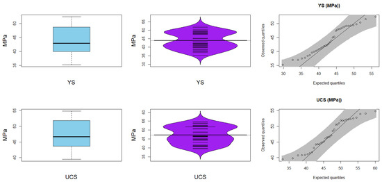
Figure 9.
Boxplot, beanplot, and QQ-plot screening for the total 3D-printed ABS specimen dataset: YS-yield strength; UCS-ultimate compressive strength.
A convenient way to attempt to estimate a factorial hierarchy without making explicit assumptions about the multiple distributional tendencies of the dataset is to adopt the Gibbs sampler approach. In Figure 10, the twelve generated posterior distributions are tiled in terms of the Gibbs sampling regression histograms for the yield strength characteristic. The posterior distribution landscape is necessary to be formed in order to proceed to estimate the central tendencies for each of the coefficients of regression (including the fixed term). In Table 13, the estimated coefficient means resulting from the Gibbs regression are listed along with their standard errors. The strength hierarchy, expressed in decreasing order, suggests the following six controlling factors: D, F, A, I, B, and K. The last three controlling factors are fairly close to each other, judging by the size of their mean coefficient magnitudes. From this active group, it is the A-factor (layer thickness) and the I-factor (use of raft) that negatively influence the yield strength response. It is remarked that the Gibbs regression screening results of the yield strength response agree both on the combination of the active effects as well as on the regression coefficient predictions with regards to the neutrosophic profiler outcomes (Table 11). The three controlling factors that stood out according to the Lenth test outcomes on the lower and upper neutrosophic yield-strength limits are also predicted in the same order by the Gibbs regression, i.e., D (infill angle), F (outline overlap), and A (layer thickness).
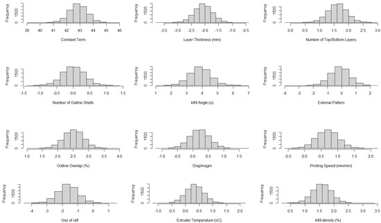
Figure 10.
Posterior distribution landscape for the multifactorial Gibbs sampler regression of the yield strength for all 36 3D-printed ABS specimens.
Table 13.
Gibbs sampler regression coefficients for all three replicates of the yield strength response.
The next question is whether a more standard regression analysis approach could approximate the predictions in congruence with the neutrosophic profiler solution. The results from the stepwise multifactorial regression analysis (IBM SPSS v. 29) of the yield strength response are tabulated in Table 14. The progressive inclusion of the active factorial terms is detailed in Table 15. From Table 14, the statistically important controlling factors are as follows: A, B, D, F, H, I, and K, and the model has a constant term (α = 0.05). If a Bonferroni family-wise error rate (α = 0.0042) is used to compensate for the multiple comparison problem, then the predictors H and I might be removed from the list. This last solution does not agree with the stepwise regression screening line-up, in which, in decreasing potency, the effects become F, A, D, B, K, I, and H (Table 15). From Table 14, it appears that there is no issue of multicollinearity in the stepwise regression treatment; the variance inflation factor for all predictors is uniform at an estimated value of 1.0. From Table 15, the adjusted R2 was estimated at 0.864, which is a satisfactory performance for this type of complex problem. Additionally, from the same table, the Durbin–Watson test statistic was estimated at 2.374, which implies that there is no autocorrelation at lag 1 between the regression residuals. In conclusion, the core predictors (F, A, and D) are alike, according to all three techniques that were employed up to this stage. It is contested, though, whether the remaining four predictors (B, K, I, and H) should all be retained on the active list. Therefore, a quantile regression analysis was also employed to screen the yield strength response by probing deeper into the regressor hierarchy against the previous predictions. From Table 16, the statistically significant regressors are A and F if the Bonferroni family-wise error rate (α = 0.0042) is applied to the estimated p-values.
Table 14.
Stepwise multifactorial regression coefficients for the combined dataset of the yield strength response (IBM SPSS v. 29).
Table 15.
Stepwise regression performance for selecting contributing factors—combined dataset of the yield strength response (IBM SPSS v. 29).
Table 16.
Quantile multifactorial regression coefficients for the combined dataset of the yield strength response.
Irrespective of the employed method, the strength of the contributions from the three more dominant factors is statistically approximated by the same regression coefficient values in the case of yield strength. For completeness, the stepwise regression analysis results for the ultimate compression strength are listed in Table 17. They confirm that the magnitudes of the regression coefficients align with those from the previous treatments for the yield strength, thus solidifying the correlation between the response behaviors of the yield strength and the ultimate compression strength. Similarly, in this case, the variance inflation factor is unity for all regressors, which assures that there might not be a multi-collinearity condition in the model. Moreover, the Durbin-Watson test statistic returns a value close to 2, which indicates that there is no autocorrelation at lag 1 between the regression residuals (Table 18). The stepwise regression screening of the ultimate compression strength response retains the same seven predictors as those found in the corresponding yield strength response model. The only noticeable difference is that factor D (infill angle), which usually joined the group of “upper-class” active regressors in the previous profiling outcomes, now enters the model in later rounds as a weaker influence (Table 18). The adjusted coefficient of determination, including the seven predictors, is estimated at 0.860, which is reasonable for this type of complex problem (Table 18).
Table 17.
Stepwise multifactorial regression coefficients for the combined dataset of the ultimate compression strength response (IBM SPSS v. 29).
Table 18.
Stepwise regression performance for selecting contributing factors—combined dataset of the ultimate compression strength response (IBM SPSS v. 29).
Even though the L12(211) OA is a linear screening design, it is perhaps worthwhile to inspect the response table of the two mechanical properties in terms of their optimal outputs. From Table 19, it is seen that the location of the maximum output for the yield strength is (1) 45.97 MPa (median = 47.83 MPa) for predictor A1 (layer thickness set at 0.1 mm), (2) 45.83 MPa (median = 46.47 MPa) for predictor D2 (infill angle set at 0°), (3) 46.41 MPa (median = 47.83 MPa) for predictor F2 (outline overlap set at 80%), (4) 45.52 MPa (median = 48.07 MPa) for predictor B2 (number of top/bottom layers set at 5), and (5) 45.50 MPa (median = 45.11 MPa) for predictor K2 (infill density set at 100%).
Table 19.
Response table for yield strength (YS) and ultimate compression strength (UCS)—normal and robust location and dispersion estimations.
Furthermore, from Table 19, it is seen that the mean location of the maximum output for the ultimate compression strength is (1) 49.35 MPa (median = 51.17 MPa) for predictor A1 (layer thickness set at 0.1 mm), (2) 48.62 MPa (median = 49.75 MPa) for predictor D2 (infill angle set at 0°), (3) 49.31 MPa (median = 47.83 MPa) for predictor F2 (outline overlap set at 80%), (4) 48.95 MPa (median = 51.38 MPa) for predictor B2 (number of top/bottom layers set at 5), and (5) 49.25 MPa (median = 48.73 MPa) for predictor K2 (infill density set at 100%). The grand mean for the ultimate compression strength dataset is 47.20 MPa (median = 46.64 MPa), and the standard error estimate is 0.80 MPa. Therefore, a predicted ultimate compression strength response is calculated at 56.68 MPa. Based on the optimal controlling factors for the 10 confirmation runs (Figure 11), the mean ultimate compression strength from the confirmation trials was estimated at 53.58 MPa (standard error = 0.29 MPa); this indicates a successful prediction since the difference between prediction and confirmation estimates is only 5.5%.
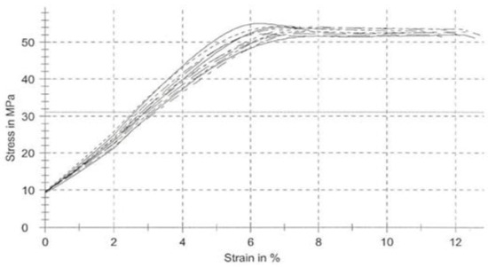
Figure 11.
Confirmation experiments of the yield strength and ultimate compression strength properties based on the optimal settings of the active controlling factors (stress-strain curves).
5. Conclusions
Lean-and-green datacentric-based experimentation may aid in accelerating the study of the mechanical properties of popular materials in modern production environments that seek to promote sustainability in product/process development/improvement. An assortment of an orthogonal trial planner with a Gibbs sampler and a neutrosophic profiler was devised to assist an additive manufacturing process to conform to sustainable research practices. The working thermoplastic material—acrylonitrile butadiene styrene (ABS)—was selected because of its wide applicability and its high recyclability. A low-cost, easily accessible 3D printer was programmed to transform ABS EVO (NEEMA 3D) filament into cubic specimens (side length of 1 cm). To examine the relevance of the product development controls to yield a sustainable unit, specimens were created by an L12(211) orthogonal trial planner, which permitted the preset manipulation of all controlling factors in the recipes while sustaining the number of 3D-printer runs and their scheduled replications to affordably low levels. This was a crucial issue because as many as eleven controlling factors were synchronously investigated. The experimental output was the two basic characteristic measurements of the 3D-printed unit, i.e., the yield strength and the ultimate compression strength responses of the ABS specimens. The trial recipes were replicated three times to ensure the viability of the screened results. The study considered the potential multi-distributional data effects, not dismissing indeterminacy issues due to the complicated physics of the mechanical tests. It was found that the yield strength and the ultimate compression strength were correlated on a replicate basis. Therefore, the factorial screening analysis that ensued was greatly simplified by focusing only on yield strength. This occurrence simplified the overall statistical engineering formulation since it reduced the initial two-response problem to a more manageable single-response case. Consequently, the neutrosophic regression approach was employed to provide the multifactorial profiling outcomes. To assess the sustainability potential of the predicted product characteristics, the screening recommendations were also interpreted by evoking the marginal, conditional, and posterior distribution features of the Gibbs sampler. Furthermore, the predictions were compared to other more ordinary multifactorial treatments, such as stepwise regression analysis and robust quantile regression. Overall, it was found that the layer thickness, the infill angle, and the outline overlap were the more dominant influences in maximizing the yield strength and the ultimate compressive strength. However, the number of top/bottom layers and the infill density could also contribute to improved performance. Even though it was a designed study that sought to identify any linear effects for screening purposes, the collected information was exploited further to test how repeatable the predictions could have been. Thus, the confirmation runs were conducted by choosing the optimal settings for the predictors, which were determined from this study: (1) the layer thickness was set at 0.1 mm, (2) the infill angle was set at 0°, (3) the outline overlap was set at 80%, (4) the number of the top/bottom layers was set at 5, and (5) the infill density was set at 100%. The performance of the optimal 3D-printed ABS specimens was adequately predictable to support the sustainability of the obtained screening solution; discrepancies were estimated at 3.5% for a confirmed mean yield strength of 51.70 MPa and at 5.5% for a confirmed mean ultimate compression strength of 53.58 MPa. Future research could involve a more complicated product-unit structure, possibly incorporating more advanced materials and composites, while monitoring additional product characteristics such as geometrical dimensions and so forth.
Author Contributions
Conceptualization, T.P. and G.B.; methodology, T.P. and G.B.; validation, T.P. and G.B.; formal analysis, G.B.; investigation, T.P.; resources, T.P. and G.B.; writing—original draft preparation, G.B.; writing—review and editing, G.B.; supervision, G.B.; project administration, G.B. All authors have read and agreed to the published version of the manuscript.
Funding
This research received no external funding.
Institutional Review Board Statement
Not applicable.
Informed Consent Statement
Not applicable.
Data Availability Statement
The data are available in the MSc thesis of Pantas in ref. [87].
Conflicts of Interest
The authors declare no conflicts of interest.
References
- Ali, M.H.; Batai, S.; Sarbassov, D. 3D printing: A critical review of current development and future prospects. Rapid Prototyp. J. 2019, 25, 1108–1126. [Google Scholar] [CrossRef]
- Jemghili, R.; Taleb, A.A.; Khalifa, M. A bibliometric indicators analysis of additive manufacturing research trends from 2010 to 2020. Rapid Prototyp. J. 2021, 27, 1432–1454. [Google Scholar] [CrossRef]
- United Nations. Sustainable Development Goals, Goal 9: Build Resilient Infrastructure, Promote Inclusive and Sustainable Industrialization and Foster Innovation. Available online: https://sdgs.un.org/goals/goal9 (accessed on 13 January 2024).
- United Nations. Sustainable Development Goals, Goal 12: Ensure Sustainable Consumption and Production Patterns. Available online: https://sdgs.un.org/goals/goal12 (accessed on 13 January 2024).
- Huang, S.H.; Liu, P.; Mokasdar, A.; Hou, L. Additive manufacturing and its societal impact: A literature review. Int. J. Adv. Manuf. Technol. 2013, 67, 1191–1203. [Google Scholar] [CrossRef]
- Gebler, M.; Schoot Uiterkamp, A.J.M.; Visser, C. A global sustainability perspective on 3D printing technologies. Energy Policy 2014, 74, 158–167. [Google Scholar] [CrossRef]
- Garg, M.; Rani, R.; Meena, V.K.; Singh, S. Significance of 3D printing for a sustainable environment. Mater. Today Sustain. 2023, 23, 100419. [Google Scholar] [CrossRef]
- Dilberoglu, U.M.; Gharehpapagh, B.; Yaman, U.; Dolen, M. The Role of Additive Manufacturing in the Era of Industry 4.0. Procedia Manuf. 2017, 11, 545–554. [Google Scholar] [CrossRef]
- Sartal, A.; Bellas, R.; Mejias, A.M.; Garcia-Collado, A. The sustainable manufacturing concept, evolution and opportunities within Industry 4.0: A literature review. Adv. Mech. Eng. 2020, 12, 1–17. [Google Scholar] [CrossRef]
- Khorasani, M.; Loy, J.; Ghasemi, A.H.; Sharabian, E.; Leary, M.; Mirafzal, H.; Cochrane, P.; Rolfe, B.; Gibson, I. A review of Industry 4.0 and additive manufacturing synergy. Rapid Prototyp. J. 2022, 28, 1462–1475. [Google Scholar] [CrossRef]
- Garcia, F.L.; da Silva Moris, V.A.; Nunes, A.O.; Silva, D.A.L. Environmental performance of additive manufacturing process—An overview. Rapid Prototyp. J. 2018, 24, 1166–1177. [Google Scholar] [CrossRef]
- Taborda, L.L.L.; Maury, H.; Pacheco, J. Design for additive manufacturing: A comprehensive review of the tendencies and limitations of methodologies. Rapid Prototyp. J. 2021, 27, 918–966. [Google Scholar] [CrossRef]
- Ngo, T.D.; Kashani, A.; Imbalzano, G.; Nguyen, K.T.Q.; Hui, D. Additive Manufacturing (3D Printing): A Review of Materials, Methods, Applications and Challenges. Compos. Part B Eng. 2018, 143, 172–196. [Google Scholar] [CrossRef]
- Gopal, M.; Lemu, H.G.; Gutema, E.M. Sustainable Additive Manufacturing and Environmental Implications: Literature Review. Sustainability 2023, 15, 504. [Google Scholar] [CrossRef]
- Peng, T.; Kellens, K.; Tang, R.; Chen, C.; Chen, G. Sustainability of additive manufacturing: An overview on its energy demand and environmental impact. Addit. Manuf. 2018, 21, 694–704. [Google Scholar] [CrossRef]
- Nadagouda, M.N.; Ginn, M.; Rastogi, V. A review of 3D printing techniques for environmental applications. Curr. Opin. Chem. Eng. 2020, 28, 173–178. [Google Scholar] [CrossRef] [PubMed]
- Tabassum, T.; Mir, A.A. A review of 3D printing technology—The future of sustainable construction. Mater. Today Proc. 2023, 93, 408–414. [Google Scholar] [CrossRef]
- Le Bourhis, F.; Kerbrat, O.; Hascoet, J.Y.; Mognol, P. Sustainable manufacturing: Evaluation and modeling of environmental impacts in additive manufacturing. Int. J. Adv. Manuf. Technol. 2013, 69, 1927–1939. [Google Scholar] [CrossRef]
- Diegel, O.; Kristav, P.; Motte, D.; Kianian, B. Additive manufacturing and its effect on sustainable design. In Handbook of Sustainability in Additive Manufacturing; Muthu, S.S., Savalani, M.M., Eds.; Springer: New York, NY, USA, 2016; Volume 1, pp. 73–99. [Google Scholar]
- Thompson, M.K.; Moroni, G.; Vaneker, T.; Fadel, G.; Campbell, R.I.; Gibson, I.; Bernard, A.; Schulz, J.; Graf, P.; Ahuja, B.; et al. Design for additive manufacturing: Trends, opportunities, considerations, and constraints. CIRP Ann. Manuf. Technol. 2016, 65, 737–760. [Google Scholar] [CrossRef]
- Yang, S.; Zhao, Y.F. Additive manufacturing-enabled design theory and methodology: A critical review. Int. J. Adv. Manuf. Technol. 2015, 80, 327–342. [Google Scholar] [CrossRef]
- Tang, Y.; Zhao, Y.F. A survey of the design methods for additive manufacturing to improve functional performance. Rapid Prototyp. J. 2016, 22, 569–590. [Google Scholar] [CrossRef]
- Suarez, L.; Dominguez, M. Sustainability and environmental impact of fused deposition modeling (FDM) technologies. Int. J. Adv. Manuf. Technol. 2020, 106, 1267–1279. [Google Scholar] [CrossRef]
- Wang, Y.; Mushtaq, R.T.; Ahmed, A.; Rehman, M.; Khan, A.M.; Sharma, S.; Ishfaq, K.; Ali, H.; Gueye, T. Additive manufacturing is sustainable technology: Citespace based bibliometric investigations of fused deposition modeling approach. Rapid Prototyp. J. 2022, 28, 654–675. [Google Scholar] [CrossRef]
- Mecheter, A.; Tarlochan, F. Fused Filament Fabrication Three-Dimensional Printing: Assessing the Influence of Geometric Complexity and Process Parameters on Energy and the Environment. Sustainability 2023, 15, 12319. [Google Scholar] [CrossRef]
- Bakhtiari, H.; Aamir, M.; Tolouei-Rad, M. Effect of 3D Printing Parameters on the Fatigue Properties of Parts Manufactured by Fused Filament Fabrication: A Review. Appl. Sci. 2023, 13, 904. [Google Scholar] [CrossRef]
- Faludi, J.; Hu, Z.; Alrashed, S.; Braunholz, C.; Kaul, S.; Kassaye, L. Does material choice drive sustainability of 3D printing? Int. J. Mech. Aerosp. Ind. Mechatron. Manuf. Eng. 2015, 9, 216–223. [Google Scholar]
- Di, L.; Yang, Y.; Wang, S. Additive manufacturing thermoplastic recycling: Profit-driven planning and optimization. J. Clean. Prod. 2024, 436, 140598. [Google Scholar] [CrossRef]
- Di, L.; Yang, Y. Towards closed-loop material flow in additive manufacturing: Recyclability analysis of thermoplastic waste. J. Clean. Prod. 2022, 362, 132427. [Google Scholar] [CrossRef]
- Madhu, N.R.; Erfani, H.; Jadoun, S.; Amir, M.; Thiagarajan, Y.; Chauhan, N.P.S. Fused deposition modelling approach using 3D printing and recycled industrial materials for sustainable environment: A review. Int. J. Adv. Manuf. Technol. 2022, 122, 2125–2138. [Google Scholar] [CrossRef]
- Sola, A.; Trinchi, A. Recycling as a Key Enabler for Sustainable Additive Manufacturing of Polymer Composites: A Critical Perspective on Fused Filament Fabrication. Polymers 2023, 15, 4219. [Google Scholar] [CrossRef]
- Golubovic, Z.; Danilov, I.; Bojovic, B.; Petrov, L.; Sedmak, A.; Miškovic, Ž.; Mitrovic, N.A. Comprehensive Mechanical Examination of ABS and ABS-like Polymers Additively Manufactured by Material Extrusion and Vat Photopolymerization Processes. Polymers 2023, 15, 4197. [Google Scholar] [CrossRef]
- Dunbar, M.A.; Dhaliwal, G.S.; Ayorinde, E.; Al-Zubi, M. Tensile, compression and flexural characteristics of acrylonitrile-butadiene-styrene at low strain rates: Experimental and numerical investigation. Polym. Polym. Compos. 2021, 29, 331–342. [Google Scholar]
- Manish; Gurjar, D.; Sharma, S.; Akash; Sarkar, M. A review on testing methods of recycled Acrylonitrile Butadiene Styrene. Mater. Today Proc. 2018, 5, 28296–28304. [Google Scholar] [CrossRef]
- Jayanth, N.; Senthil, P.; Prakash, C. Effect of chemical treatment on tensile strength and surface roughness of 3D-printed ABS using the FDM process. Virtual Phys. Protot. 2018, 13, 155–163. [Google Scholar] [CrossRef]
- Mushtaq, R.T.; Iqbal, A.; Wang, Y.; Cheok, Q.; Abbas, S. Parametric effects of fused filament fabrication approach on surface roughness of acrylonitrile butadiene styrene and nylon-6 polymer. Materials 2022, 15, 5206. [Google Scholar] [CrossRef] [PubMed]
- Zohdi, N.; Nguyen, P.Q.K.; Yang, R. Evaluation on Material Anisotropy of Acrylonitrile Butadiene Styrene Printed via Fused Deposition Modelling. Appl. Sci. 2024, 14, 1870. [Google Scholar] [CrossRef]
- Kim, H.; Lin, Y.; Tseng, T.-L.B. A review on quality control in additive manufacturing. Rapid Prototyp. J. 2018, 24, 645–669. [Google Scholar] [CrossRef]
- Gordelier, T.J.; Thies, P.R.; Turner, L.; Johanning, L. Optimising the FDM additive manufacturing process to achieve maximum tensile strength: A state-of-the-art review. Rapid Prototyp. J. 2019, 25, 953–971. [Google Scholar] [CrossRef]
- Tang, Y.; Mak, K.; Zhao, Y.F. A framework to reduce product environmental impact through design optimization for additive manufacturing. J. Clean. Prod. 2016, 137, 1560–1572. [Google Scholar] [CrossRef]
- Chohan, J.S.; Kumar, R.; Yadav, A.; Chauhan, P.; Singh, S.; Sharma, S.; Li, C.; Dwivedi, S.P.; Rajkumar, S. Optimization of FDM printing process parameters on surface finish, thickness, and outer dimension with ABS polymer specimens using Taguchi orthogonal array and genetic algorithms. Math. Probl. Eng. 2022, 2022, 2698845. [Google Scholar] [CrossRef]
- Rajarajeswari, C.; Anbalagan, C. Integration of the green and lean principles for more sustainable development: A case study. Mater. Today Proc. 2023, in press. [Google Scholar] [CrossRef]
- Yadav, Y.; Kaswan, M.S.; Gahlot, P.; Duhan, R.K.; Garza-Reyes, J.A.; Rathi, R.; Chaudhary, R.; Yadav, G. Green Lean Six Sigma for sustainability improvement: A systematic review and future research agenda. Int. J. Lean Six Sigma 2023, 14, 759–790. [Google Scholar] [CrossRef]
- Yadav, S.; Samadhiya, A.; Kumar, A.; Majumdar, A.; Garza-Reyes, J.A.; Luthra, S. Achieving the sustainable development goals through net zero emissions: Innovation-driven strategies for transitioning from incremental to radical lean, green and digital technologies. Resour. Conserv. Recycl. 2023, 197, 107094. [Google Scholar] [CrossRef]
- Elemure, I.; Dhakal, H.N.; Leseure, M.; Radulovic, J. Integration of Lean Green and Sustainability in Manufacturing: A Review on Current State and Future Perspectives. Sustainability 2023, 15, 10261. [Google Scholar] [CrossRef]
- Womack, J.P.; Jones, D.T. Lean Thinking—Banish Waste and Create Wealth in Your Corporation; Simon and Schuster: New York, NY, USA, 1996. [Google Scholar]
- Juma, L.; Zimon, D.; Ikram, M.; Madzik, P. Towards a sustainability paradigm; the nexus between lean green practices, sustainability-oriented innovation and triple bottom line. Int. J. Prod. Econ. 2022, 245, 108393. [Google Scholar] [CrossRef]
- Fercoq, A.; Lamouri, S.; Carbone, V. Lean/Green integration focused on waste reduction techniques. J. Clean. Prod. 2016, 137, 567–578. [Google Scholar] [CrossRef]
- Marco-Ferreira, A.; Stefanelli, N.O.; Seles, B.M.R.P.; Fidelis, R. Lean and green: Practices, paradigms and future prospects. Benchmarking 2020, 27, 2077–2107. [Google Scholar] [CrossRef]
- Dieste, M.; Panizzolo, R.; Garza-Reyes, J.A.; Anosike, A. The relationship between lean and environmental performance: Practices and measures. J. Clean. Prod. 2019, 224, 120–131. [Google Scholar] [CrossRef]
- Bhattacharya, A.; Nand, A.; Castka, P. Lean-green integration and its impact on sustainability: A critical review. J. Clean. Prod. 2019, 236, 117697. [Google Scholar] [CrossRef]
- Kaswan, M.S.; Rathi, R.; Garza-Reyes, J.A.; Antony, J. Green lean six sigma sustainability-oriented project selection and implementation framework for manufacturing industry. Int. J. Lean Six Sigma 2023, 14, 33–71. [Google Scholar] [CrossRef]
- Rathi, R.; Kaswan, M.S.; Garza-Reyes, J.A.; Antony, J.; Cross, J. Green lean six sigma for improving manufacturing sustainability: Framework development and validation. J. Clean. Prod. 2022, 345, 131130. [Google Scholar] [CrossRef]
- Chugani, N.; Kumar, V.; Garza-Reyes, J.A.; Rocha-Lona, L.; Upadhyay, A. Investigating the green impact of lean, six sigma and lean six sigma: A systematic literature review. Int. J. Lean Six Sigma 2017, 8, 7–32. [Google Scholar] [CrossRef]
- Fisher, R.A. Statistical Methods, Experimental Design, and Scientific Inference; Oxford University Press: Oxford, UK, 1990. [Google Scholar]
- Hoerl, R.W.; Snee, R.D. Guiding beacon: Using statistical engineering principles for problem solving. Qual. Prog. 2015, 48, 52–54. [Google Scholar]
- Hare, L.B. Statistics spotlight: The foundation of statistical engineering. Qual. Prog. 2019, 52, 48–51. [Google Scholar]
- Anderson-Cook, C.M.; Lu, L.; Brenneman, W.; De Mast, J.; Faltin, F.; Freeman, L.; Guthrie, W.; Hoerl, R.; Jensen, W.; Jones-Farmer, A.; et al. Statistical engineering-Part 1: Past and present. Qual. Eng. 2022, 34, 426–445. [Google Scholar] [CrossRef]
- Anderson-Cook, C.M.; Lu, L.; Brenneman, W.; De Mast, J.; Faltin, F.; Freeman, L.; Guthrie, W.; Hoerl, R.; Jensen, W.; Jones-Farmer, A.; et al. Statistical engineering-Part 2: Future. Qual. Eng. 2022, 34, 446–467. [Google Scholar] [CrossRef]
- Schall, S. Statistical engineering: Synergies with established engineering disciplines. Qual. Eng. 2022, 34, 468–472. [Google Scholar] [CrossRef]
- Box, G.E.P.; Hunter, W.G.; Hunter, J.S. Statistics for Experimenters—Design, Innovation, and Discovery; Wiley: New York, NY, USA, 2005. [Google Scholar]
- Taguchi, G.; Chowdhury, S.; Wu, Y. Quality Engineering Handbook; Wiley: Hoboken, NJ, USA, 2004. [Google Scholar]
- Taguchi, G.; Chowdhury, S.; Taguchi, S. Robust Engineering: Learn How to Boost Quality while Reducing Costs and Time to Market; McGraw-Hill: New York, NY, USA, 2000. [Google Scholar]
- Zadeh, L.A. Fuzzy sets. Inf. Control 1965, 8, 338–353. [Google Scholar] [CrossRef]
- Priest, G. Paraconsistency and Dialetheism. In Handbook of the History of Logic: The Many Valued and Nonmonotonic: Turn in Logic; Gabbay, D.M., Woods, J., Eds.; Elsevier: Amsterdam, The Netherlands, 2007; Volume 8, pp. 129–204. [Google Scholar]
- Heyting, A. Intuitionistic views on the nature of mathematics. Synthese 1974, 27, 79–91. [Google Scholar] [CrossRef]
- Kleene, S.C. On the interpretation of intuitionistic number theory. J. Symb. Log. 1945, 10, 109–124. [Google Scholar] [CrossRef]
- Smarandache, F. Symbolic Neutrosophic Theory; EuropaNova: Bruxelles, Belgium, 2015. [Google Scholar]
- Smarandache, F. A Unifying Field in Logics. Neutrosophy: Neutrosophic Probability, Set and Logic; American Research Press: Rehoboth, DE, USA, 1999. [Google Scholar]
- Smarandache, F. Introduction to Neutrosophic Statistics; Sitech and Education Publishing: Columbus, OH, USA, 2014. [Google Scholar]
- Smarandache, F. Neutrosophic logic—A generalization of the intuitionistic fuzzy logic. In Multispace & Multistructure. Neutrosophic Transdisciplinarity; Smarandache, F., Ed.; North-European Scientific Publishers: Hanko, Finland, 2010; Volume 4, pp. 403–409. [Google Scholar]
- Atanassov, K.T. Intuitionistic fuzzy sets. Fuzzy Set. Syst. 1986, 20, 87–96. [Google Scholar] [CrossRef]
- Aslam, M. Neutrosophic analysis of variance: Application to university students. Complex Intell. Syst. 2019, 5, 403–407. [Google Scholar] [CrossRef]
- Nagarajan, D.; Broumi, S.; Smarandache, F.; Kavikumar, J. Analysis of neutrosophic multiple regression. Neutrosophic Sets Syst. 2021, 43, 44–52. [Google Scholar]
- Aslam, M. Analysis of imprecise measurement data utilizing z-test for correlation. J. Big Data 2023, 11, 1–10. [Google Scholar] [CrossRef]
- Wahab, A.; Ali, J.; Riaz, M.B.; Asjad, M.I.; Muhammad, T. A novel probabilistic q-rung orthopair linguistic neutrosophic information-based method for rating nanoparticles in various sectors. Sci. Rep. 2024, 14, 5738. [Google Scholar] [CrossRef] [PubMed]
- Ali, A.M.; Abdel-Basset, M.; Abouhawwash, M.; Gharib, M.; Mohamed, M. N-type-2-ARAS: An efficient hybrid multi-criteria optimization approach for end-of-life vehicle’s recycling facility location: A sustainable approach. Expert Syst. Appl. 2024, 250, 123873. [Google Scholar] [CrossRef]
- Irvanizam, I.; Zahara, N. An improved RAFSI method based on single-valued trapezoidal neutrosophic number and its Harmonic and Arithmetic mean operators for healthcare service quality evaluation. Expert Syst. Appl. 2024, 248, 123343. [Google Scholar] [CrossRef]
- Guo, Y.; Shahin, A.I.; Garg, H. An indeterminacy fusion of encoder-decoder network based on neutrosophic set for white blood cells segmentation. Expert Syst. Appl. 2024, 246, 123156. [Google Scholar] [CrossRef]
- Sharma, M.K.; Chaudhary, S.; Kumar, S.; Malik, A.K.; Saha, A.K. A three-dimensional probabilistic fermatean neutrosophic hesitant green transportation system for sustainable management of biomedical waste. Eng. Appl. Artif. Intell. 2024, 133, 108383. [Google Scholar] [CrossRef]
- Chen, J.; Ye, J.; Du, S. Scale effect and anisotropy analyzed for neutrosophic numbers of rock joint roughness coefficient based on neutrosophic statistics. Symmetry 2017, 9, 208. [Google Scholar] [CrossRef]
- Chen, J.; Ye, J.; Du, S.; Yong, R. Expressions of rock joint roughness coefficient using neutrosophic interval statistical numbers. Symmetry 2017, 9, 123. [Google Scholar] [CrossRef]
- Essameldin, R.; Ismail, A.A.; Darwish, S.M. An opinion mining approach to handle perspectivism and ambiguity: Moving toward neutrosophic logic. IEEE Access 2022, 10, 63314–63328. [Google Scholar] [CrossRef]
- Geman, S.; Geman, D. Stochastic relaxation, Gibbs distributions, and the Bayesian restoration of images. IEEE Trans. Pattern Anal. Mach. Intell. 1984, 6, 721–741. [Google Scholar] [CrossRef] [PubMed]
- Zeger, S.; Rizaul Karim, M. Generalized linear models with random effects: A Gibbs sampling approach. J. Am. Stat. Assc. 1991, 86, 79–86. [Google Scholar] [CrossRef]
- Casella, G.; George, E.I. Explaining the Gibbs sampler. Am. Stat. 1992, 46, 167–174. [Google Scholar] [CrossRef]
- Pantas, T. Taguchi Analysis on the Compression Properties of Acrylonitrile Butadiene Styrene (ABS) in a 3D Printing Process. Master’s Thesis, Kingston University, London, UK, 2018. [Google Scholar]
- R Core Team. R (Version 4.3.0): A Language and Environment for Statistical Computing; R Foundation for Statistical Computing: Vienna, Austria, 2023; Available online: https://www.R-project.org/ (accessed on 21 April 2023).
- Mantz, A.B. A Gibbs sampler for multivariate linear regression. arXiv 2016, arXiv:1509.00908. [Google Scholar] [CrossRef]
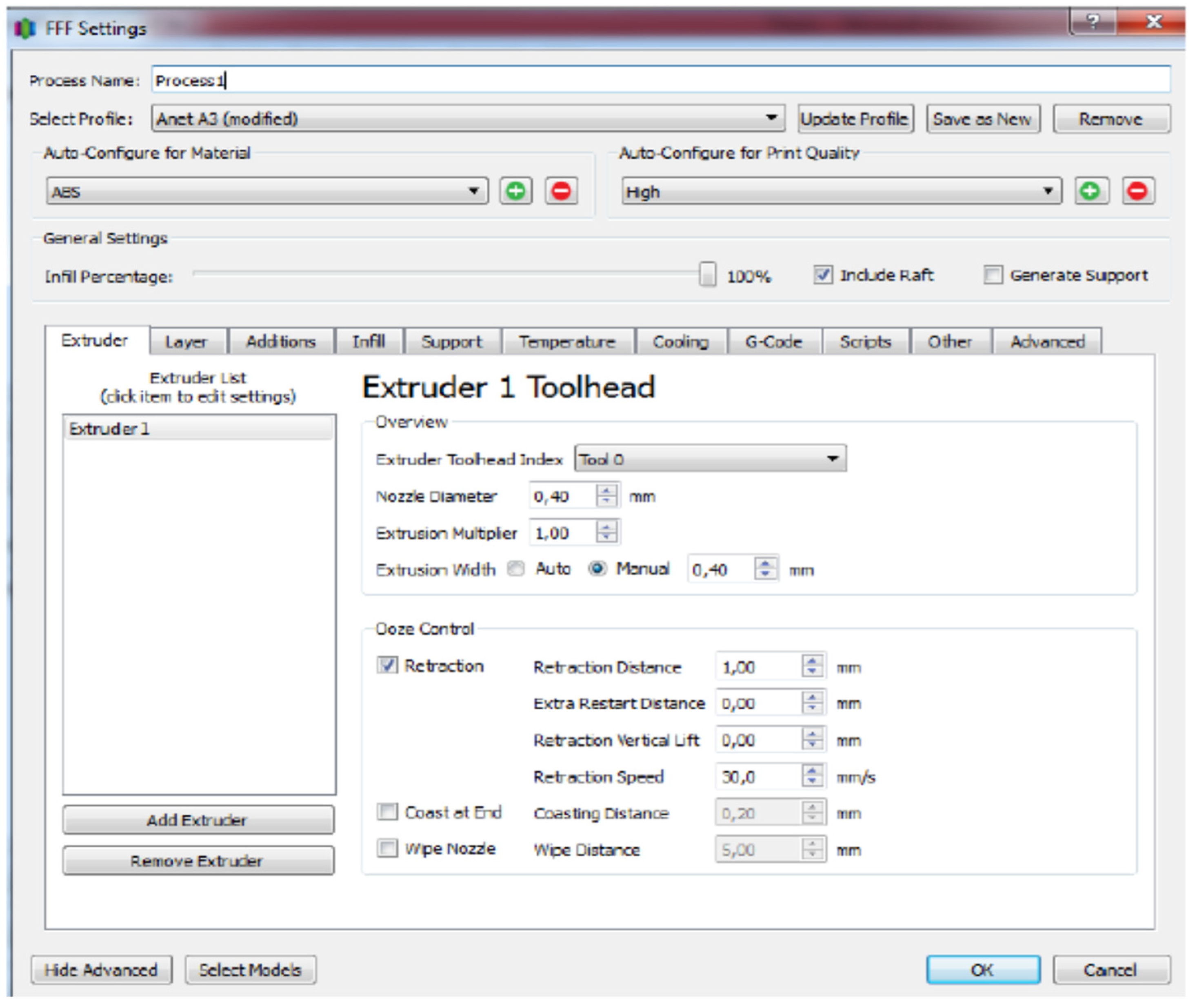

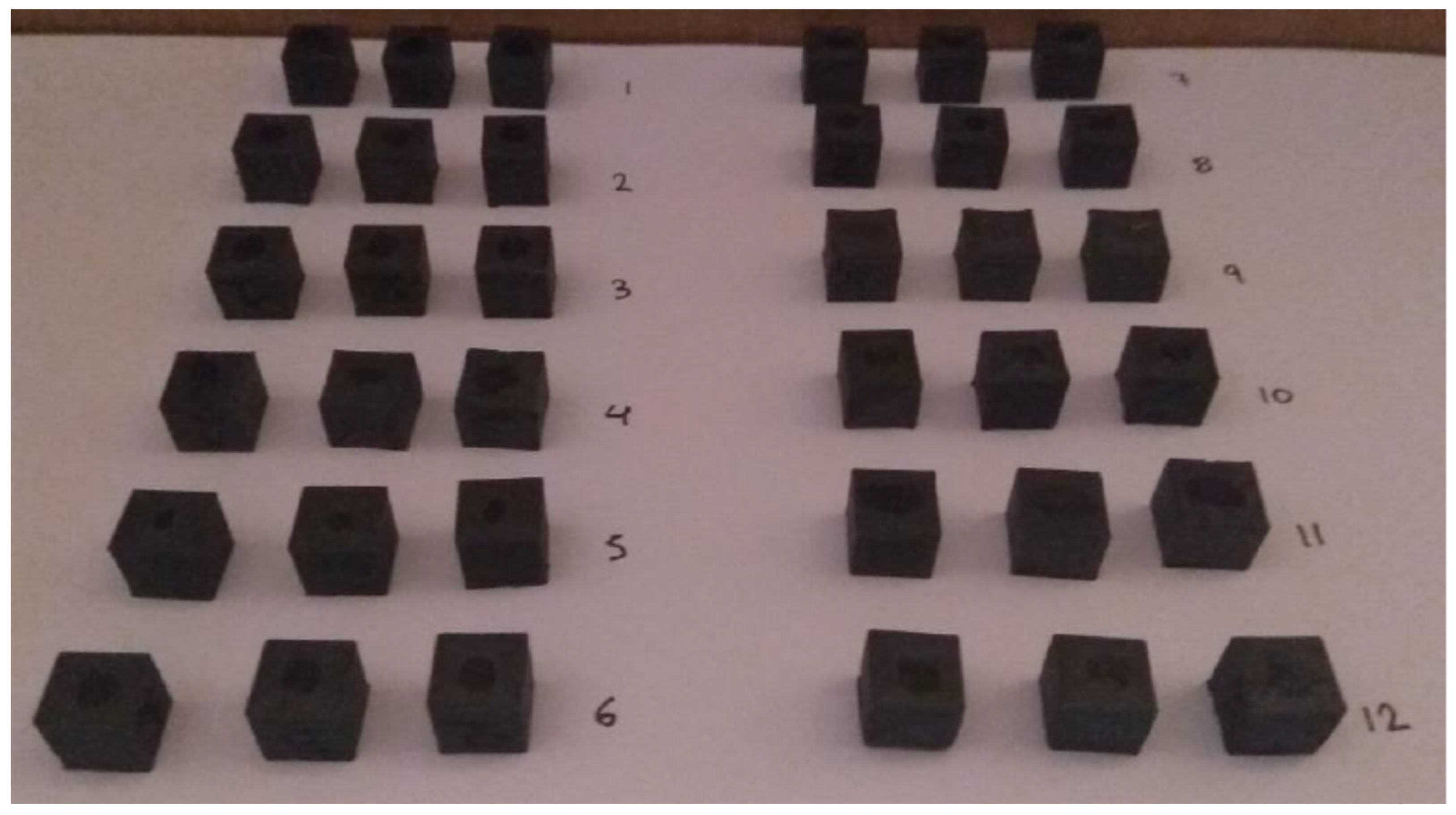
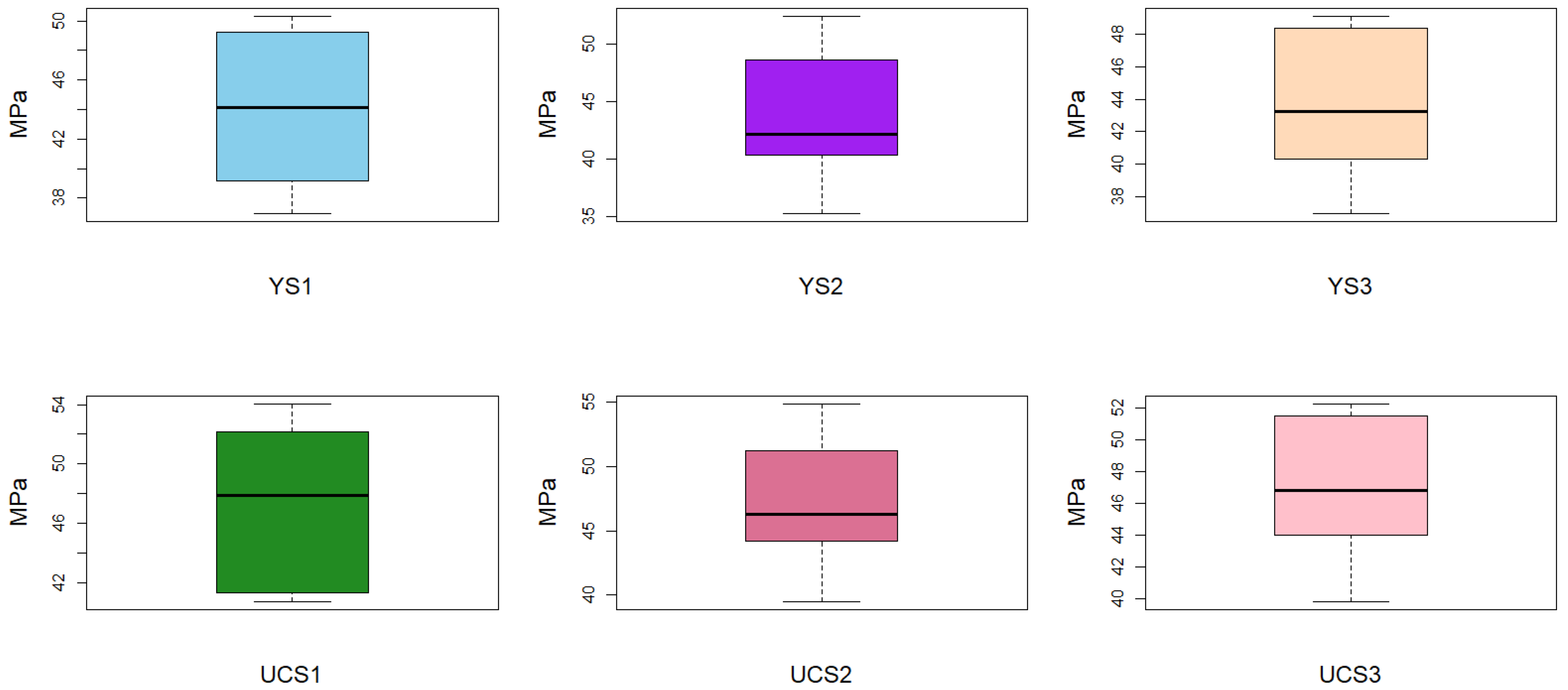
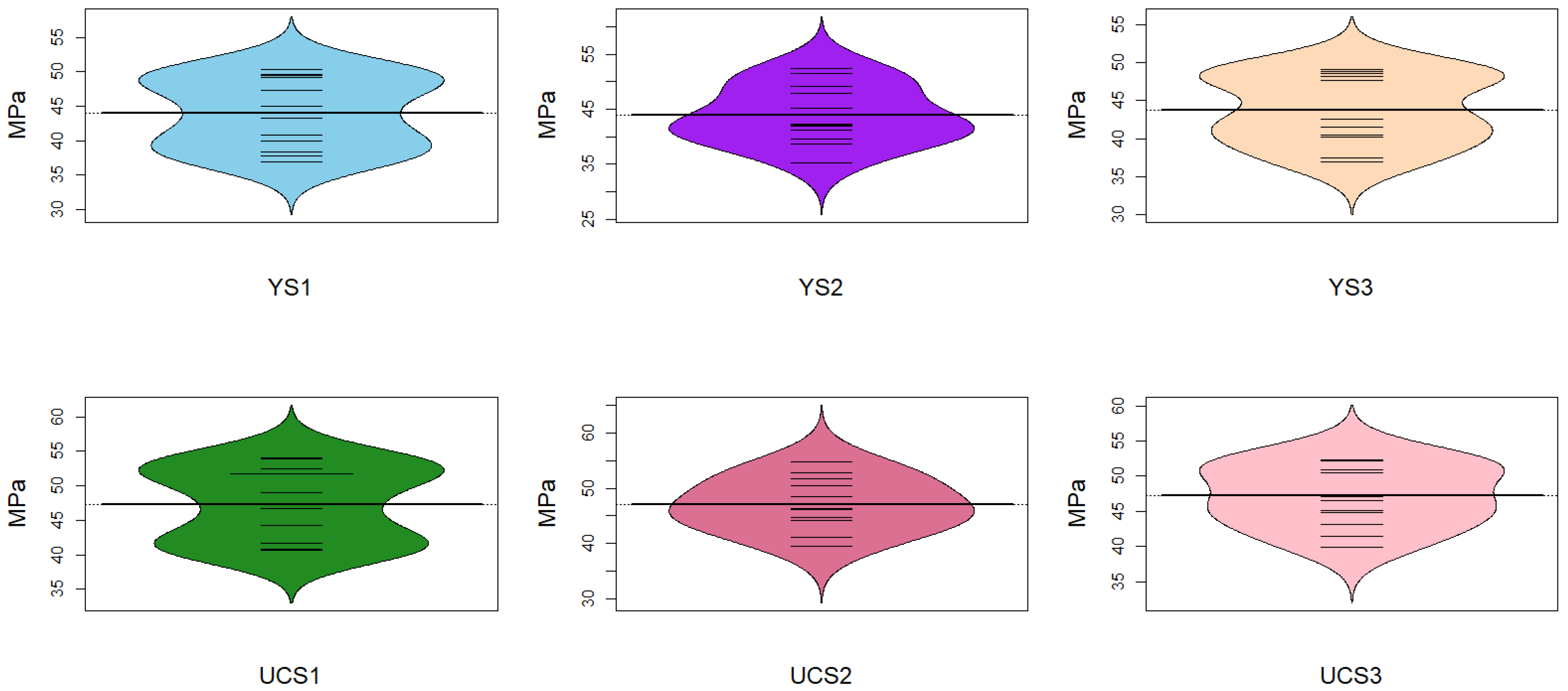
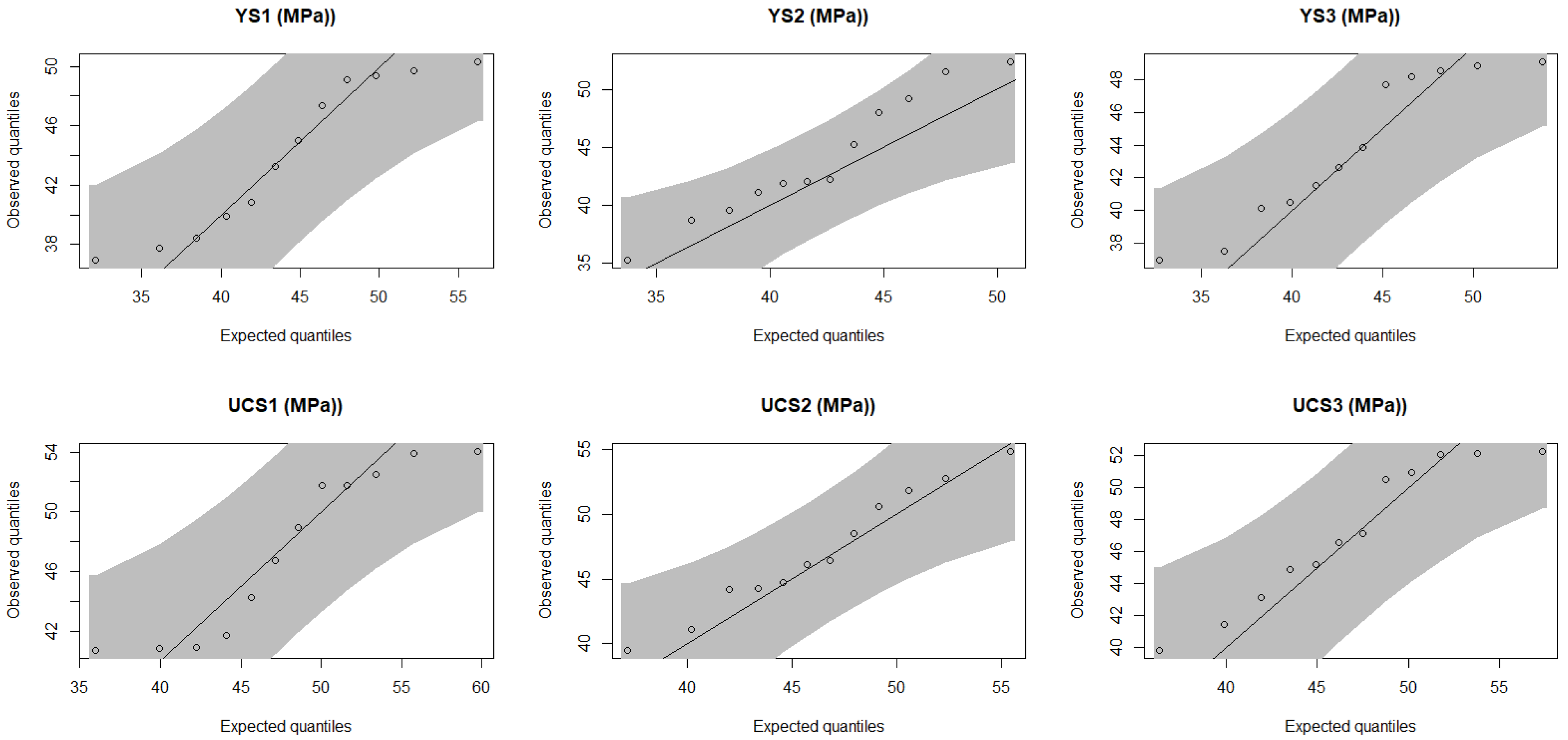
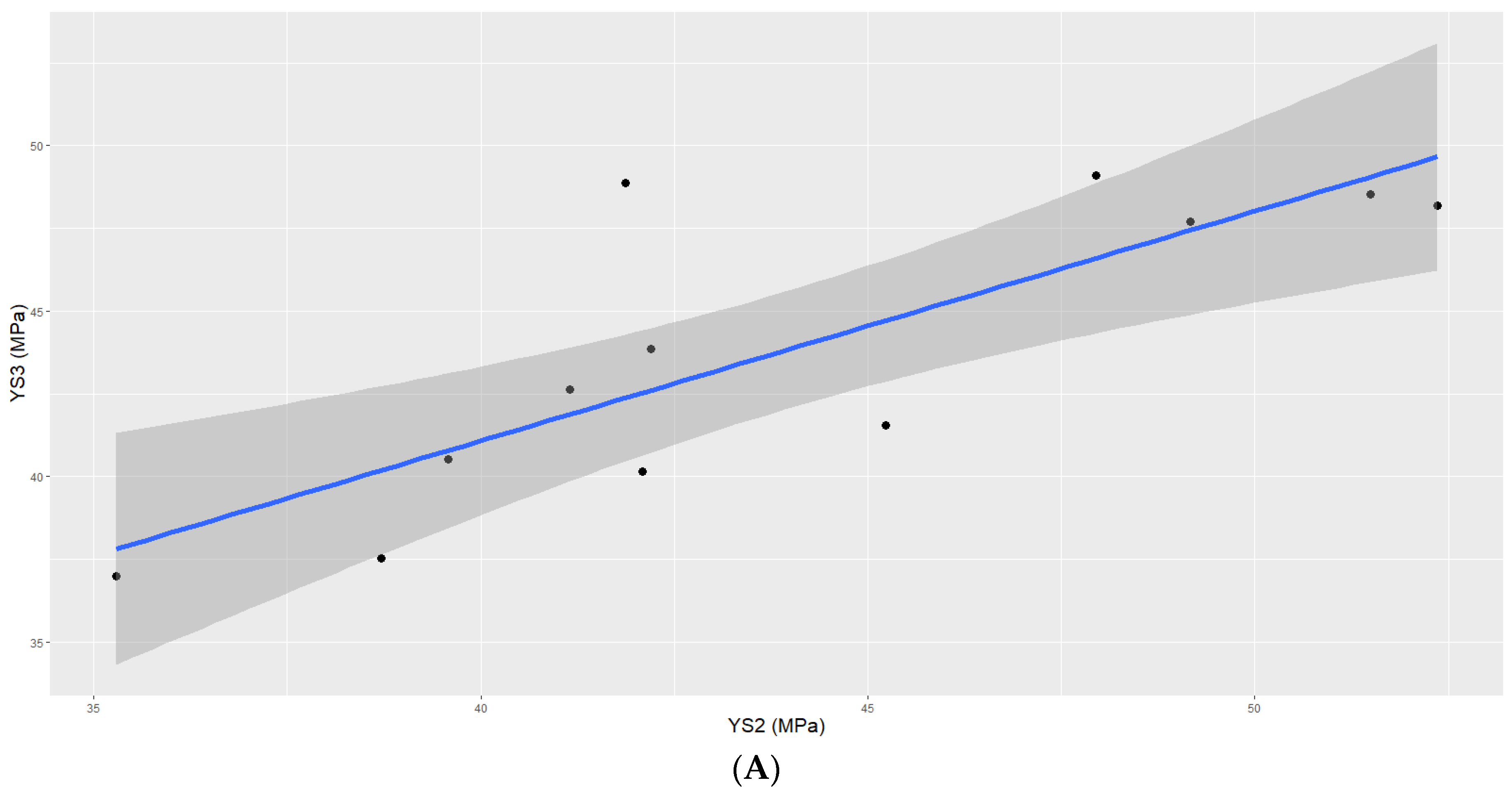
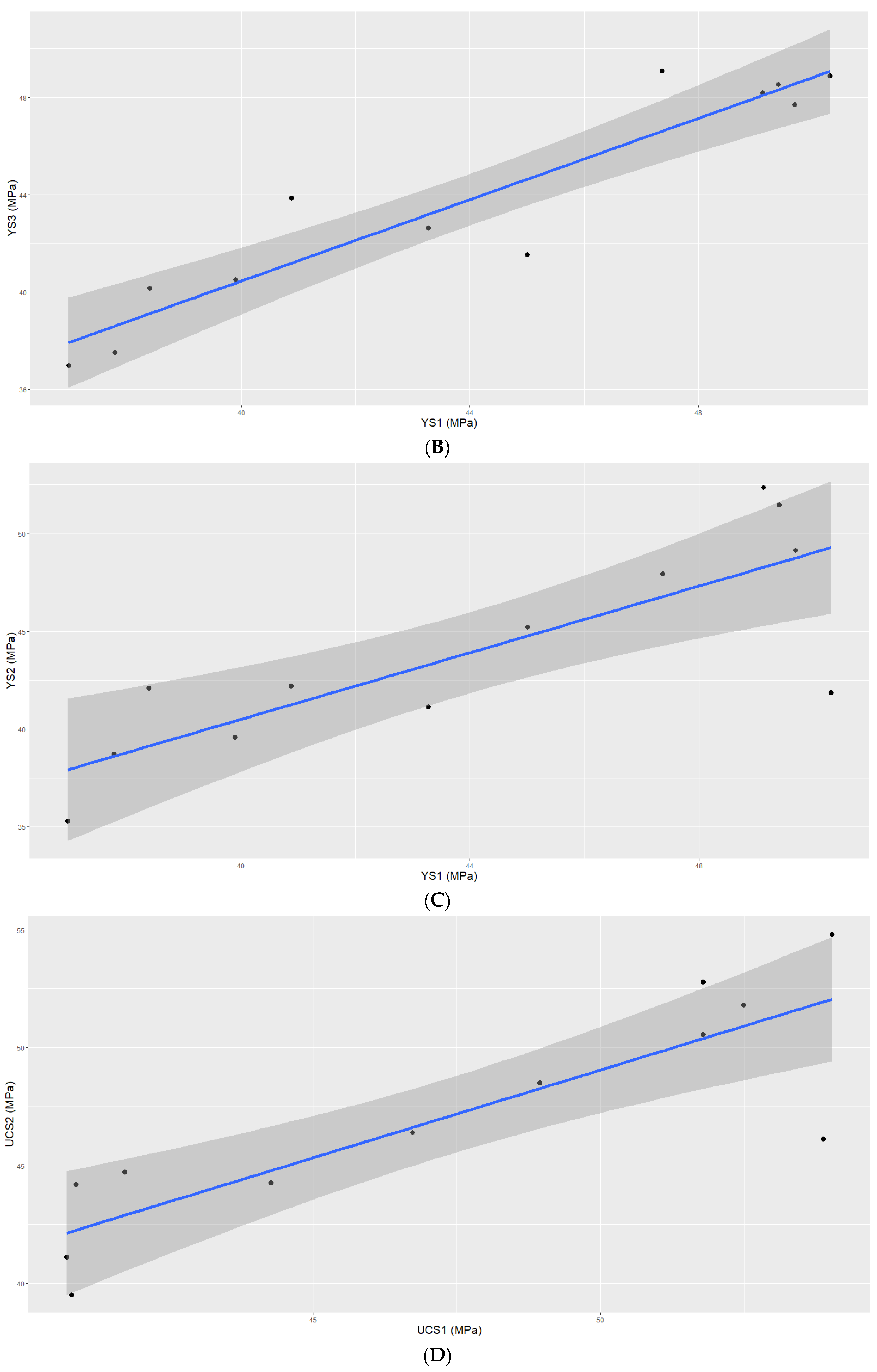
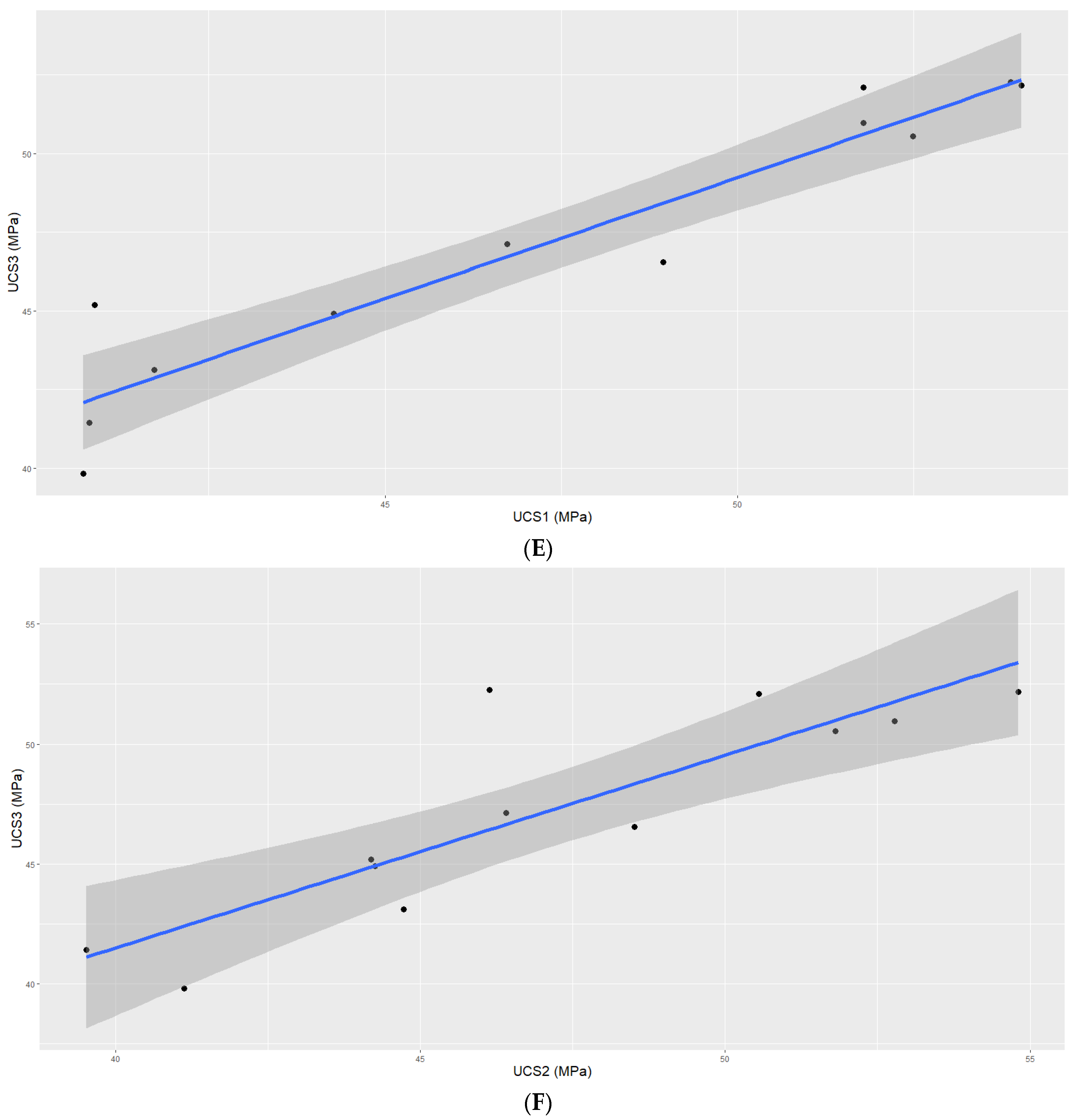


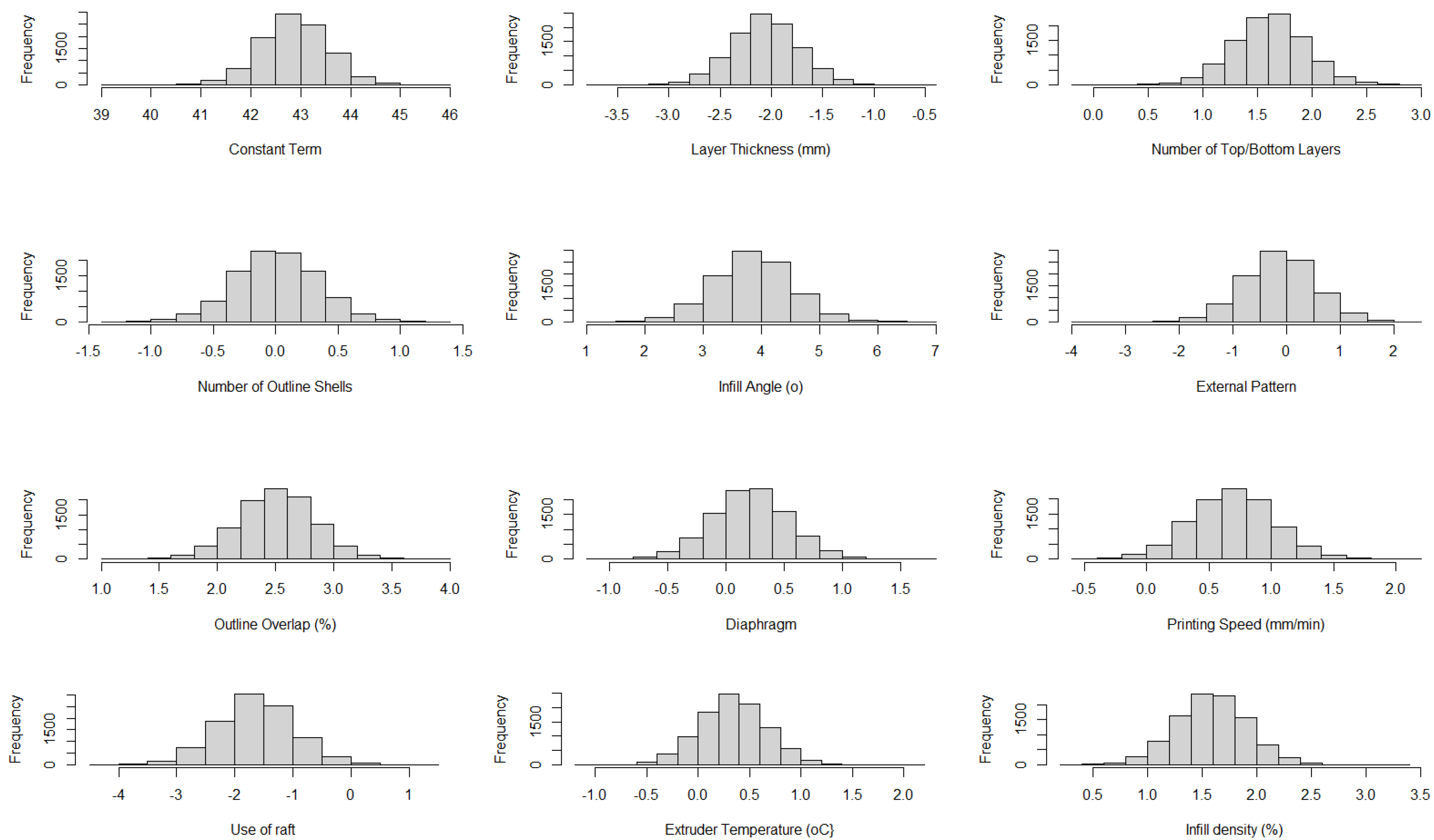
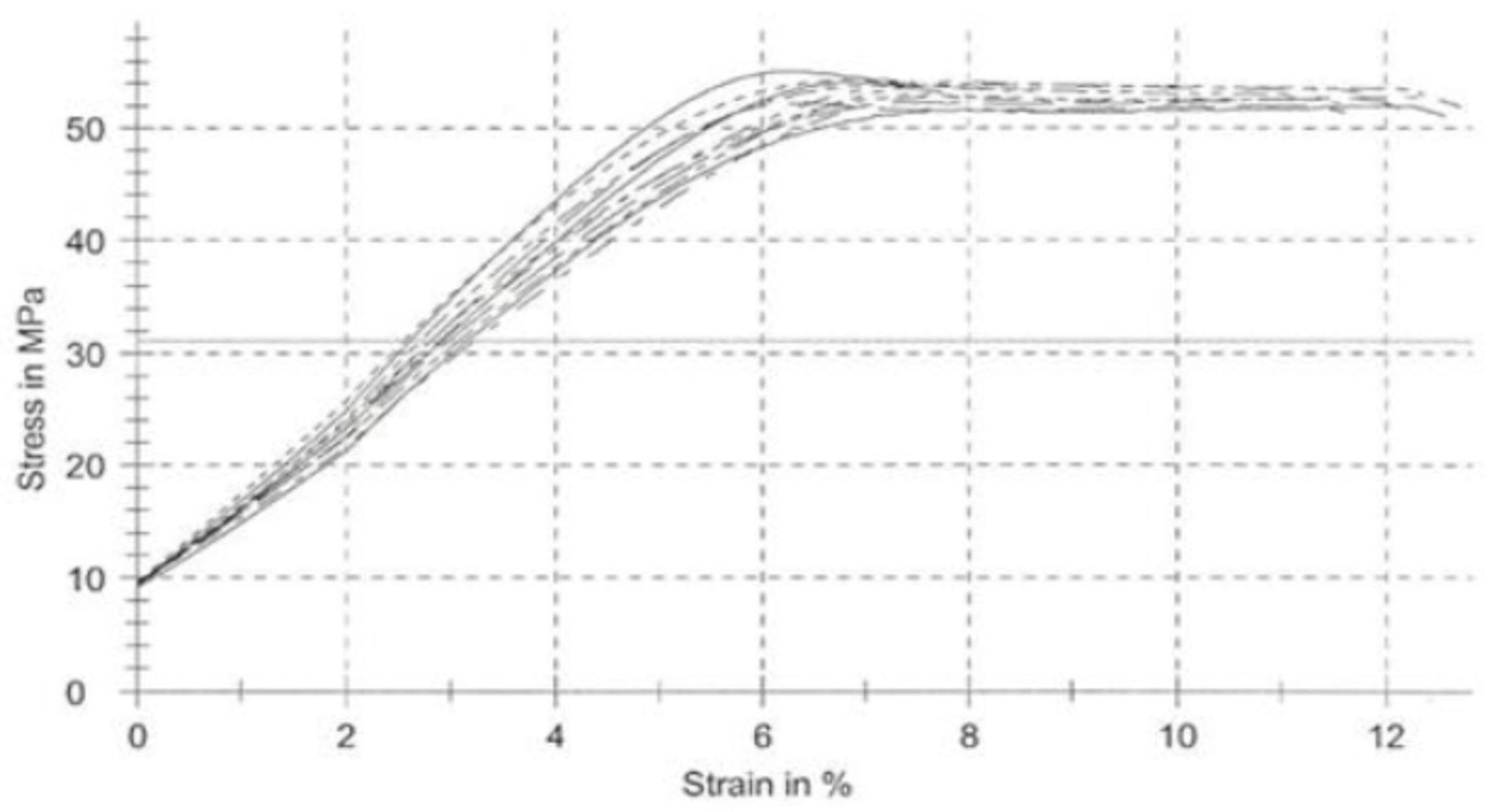
Disclaimer/Publisher’s Note: The statements, opinions and data contained in all publications are solely those of the individual author(s) and contributor(s) and not of MDPI and/or the editor(s). MDPI and/or the editor(s) disclaim responsibility for any injury to people or property resulting from any ideas, methods, instructions or products referred to in the content. |
© 2024 by the authors. Licensee MDPI, Basel, Switzerland. This article is an open access article distributed under the terms and conditions of the Creative Commons Attribution (CC BY) license (https://creativecommons.org/licenses/by/4.0/).