Real-Time Elemental Analysis Using a Handheld XRF Spectrometer in Scanning Mode in the Field of Cultural Heritage

Abstract

An X-ray fluorescence handheld spectrometer (hh-XRF) is adapted for real-time qualitative and quantitative elemental analysis in scanning mode for applications in cultural heritage. Specifically, the Tracer-5i (Bruker) is coupled with a low-cost constructed computer-controlled x–y target stage that enables the remote control of the target’s movement under the ionizing X-ray beam. Open-source software synchronizes the spectrometer’s measuring functions and handles data acquisition and data analysis. The spectrometer’s analytical capabilities, such as sensitivity, energy resolution, beam spot size, and characteristic transition intensity as a function of the distance between the spectrometer and the target, are evaluated. The XRF scanner’s potential in real-time imaging, object classification, and quantitative analysis in cultural heritage-related applications is explored and the imaging capabilities are tested by scanning a 19th-century religious icon. The elemental maps provide information on used pigments and reveal an underlying icon. The scanner’s capability to classify metallic objects was verified by analyzing the measured raw spectra of a coin collection using Principal Components Analysis. Finally, the handheld’s capability to perform quantitative analysis in scanning mode is demonstrated in the case of precious metals, applying a pre-installed quantification routine.

1. Introduction

Cultural heritage preservation demands that it be protected in a sustainable way that meets current needs and ensures future generations can do the same. The act encompasses several factors, including the use of non-destructive, non-invasive, and green diagnostic techniques. XRF fulfills all these requirements and, as a multi-elemental analytical technique, allows the elemental composition analysis of cultural artifacts. In turn, the knowledge of the elemental composition allows the extraction of information about the used materials, manufacturing techniques, structure, previous interventions, state of preservation, and the selection of effective conservation methods. Elemental analysis of artifacts with XRF can verify their authenticity and provenance, aiding in distinguishing original works. XRF scanning spectroscopy is increasingly used in cultural heritage [1,2,3,4]. It allows the noninvasive extraction of elemental information from objects with spatial heterogeneity along the surface.

In the present work, an X-ray fluorescence scanner was developed by coupling the widely used Bruker Tracer 5i XRF handheld spectrometer with a low-cost automated x–y motion control system for applications in cultural heritage [5]. The Tracer has been utilized in scanning by commercial systems moving either the handheld [6] or the sample [7,8], or even manually following points on a grid [9]. This work presents a cost-effective adaptation of Tracer 5i for real-time qualitative and quantitative elemental analysis in scanning mode. A Python-based control program offers an intuitive interface for operating the scanner and enabling handheld remote control. The scanner’s analytical capabilities are examined thoroughly. The measured spectra are analyzed in real time, allowing for immediate insights and adjustments. Three case studies illustrate the scanner’s efficiency and functionality for imaging, object classification, and quantitative analysis, demonstrating its notable performance. The imaging capabilities of the XRF scanner were tested by studying a religious icon. Elemental maps were extracted, and based on the assessment of the detected elements’ distribution, conclusions regarding the employed pigments were extracted. The scanner’s ability to classify objects is demonstrated by measuring a set of contemporary coins in scanning mode. The coins are automatically categorized into distinct clusters based on their composition through real-time evaluation of the raw spectra using Principal Component Analysis. Finally, the scanner’s ability for quantitative analysis is demonstrated by studying a set of precious alloys.

2. The X-ray Fluorescence Scanner

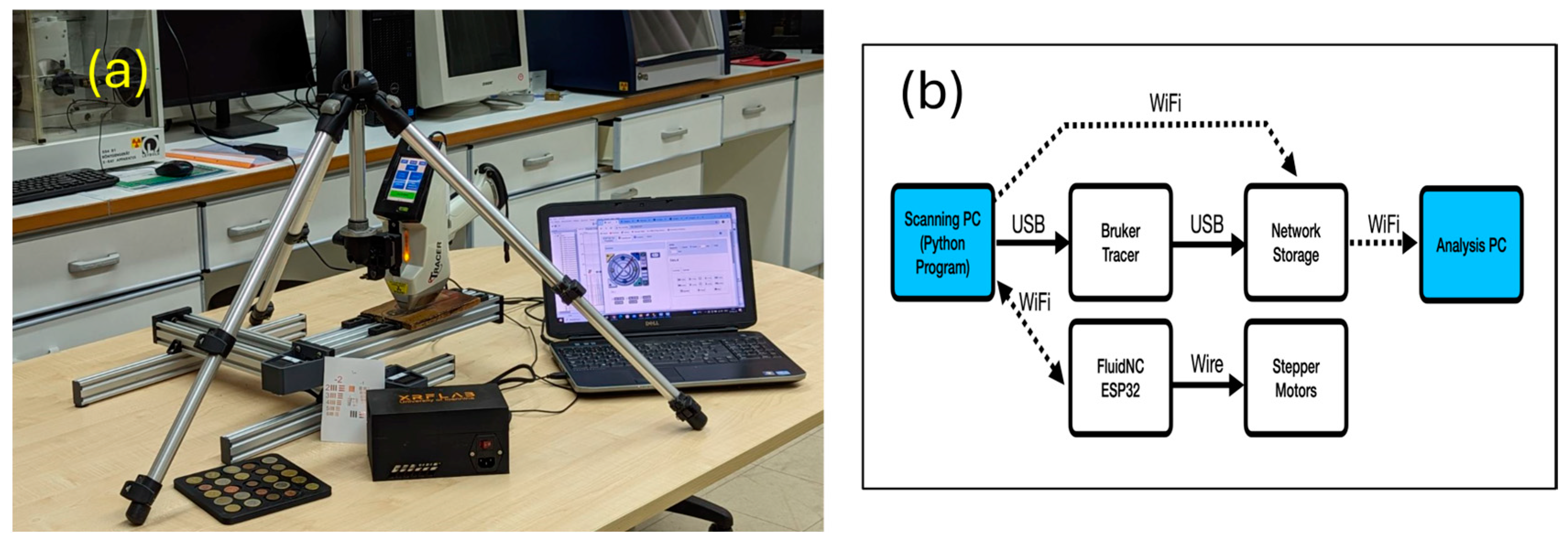
2.1. The Scanner

The XRF scanner consists of Bruker’s Tracer 5i handheld spectrometer mounted on a tripod and the sample’s two-dimensional remote-controlled motion system. Figure 1a shows the system’s high-level components, while its topology is shown in Figure 1b.

Bruker’s Tracer-5i handheld XRF spectrometer is equipped with an Rh-target X-ray tube. It can operate within a voltage range of 6 to 50 kV and a current range of 4.5 to 195 μA, with a maximum output of 4 Watts. The generated beam is collimated by two collimators, with nominal spot sizes of 3 and 8 mm. Additionally, a custom-made bronze collimator with a cylindrical bore hole of 1 mm size was constructed to improve the spatial resolution. The spectrometer’s measuring plane, for in-touch measurement, is about 30 mm away from the X-ray tube. The ionization beam impinges on the target at an angle of approximately 45° with respect to the target’s vertical axis. The detector is about 8–9 mm from the spectrometer’s measuring plane, and its active area is 20 mm². The outgoing X-ray photons towards the detector center form an angle of about 27° to the target’s vertical axis. The spectrometer has a 5-position primary beam filter changer wheel with preinstalled filters that can be changed automatically [10].

The handheld is coupled with a remote-controlled x–y stage. The motion system comprises low-cost x- and y-linear stages driven by 1.8-degree/step stepper motors. These stages have a resolution of 3 μm, allowing for precise positioning of samples in two dimensions. The scanning procedure is initiated by the user, who provides the scanning parameters, such as the number of steps and step size in each direction, and the measuring time. The maximum scanning range is 100 mm, with a minimum step size of 100 μm, in both x- and y-directions. The spectrometer’s operation parameters impose a minimum measuring time of 1 s per point.

The apparatus control program is running on the “Scanning” workstation. The control program, written in Python (version 3.11.0), accepts and validates user commands. It then (a) sends g-code motion commands [11] to the motion controller via Web Sockets for two-dimensional positioning movement and (b) triggers the Tracer 5i to initiate the measurement through Bruker’s remote application using the PyWinAuto Python library [12]. In addition, the Python program verifies the connectivity between the workstation and the motion controller, ensuring smooth communication and the correct timing of the motion and triggering actions.

The ESP32 Wroom microprocessor is used as the controller for the motion control system [13]. The motion control system is managed by FluidNC (version 3.7.0), an open-source motion control software that is accessible through a web interface [14]. FluidNC receives positional g-codes from the control program via Wi-Fi and generates step and direction pulses. After amplification, the pulses drive the stepper motors, which actuate the ball screws that move the specimen to the requested coordinates for scanning. After each single-point XRF measurement, the application verifies the successful completion of the action and confirms correct data collection and data storage. If any issues are detected, appropriate error-handling procedures are implemented. The cycle repeats until all specified scanning points have been measured. The specimen is fixtured to the x–y stage with the help of custom 3D-printed parts.

2.2. Data Handling—Data Analysis

The “Analysis” workstation coordinates the data analysis process through a Python-powered integrated workflow. A Python script, leveraging the wget module [15], initiates an HTTP GET request to download XRF spectra from the designated network address and store them locally. The script also periodically monitors the specified remote folder, synchronized with the measurement time parameter, ensuring timely acquisition of newly available spectra. This streamlines data acquisition and reduces human error.

A custom Python module has also been developed to convert binary data into a readable format. This module decodes Bruker’s binary “pdz” files into ASCII format to facilitate subsequent analysis and interpretation of the spectral data. Following conversion, the data are seamlessly transferred to an in-house open-source Python software suite (version 3.11.0), enabling functionalities such as real-time analysis of the measured XRF spectra, the creation of elemental distribution maps based on range of interest method (ROI), and monitoring of the spectrometer’s operational data (e.g., temperature, dead time) recorded during the measurement process and displayed in real time. Furthermore, the software employs Principal Component Analysis (PCA) to reduce dimensionality and visualize analytical results. This integrated workflow expedites applying rigorous analytical procedures, fostering accelerated scientific exploration and enabling informed decision making.

3. Analytical Capabilities of the Scanner

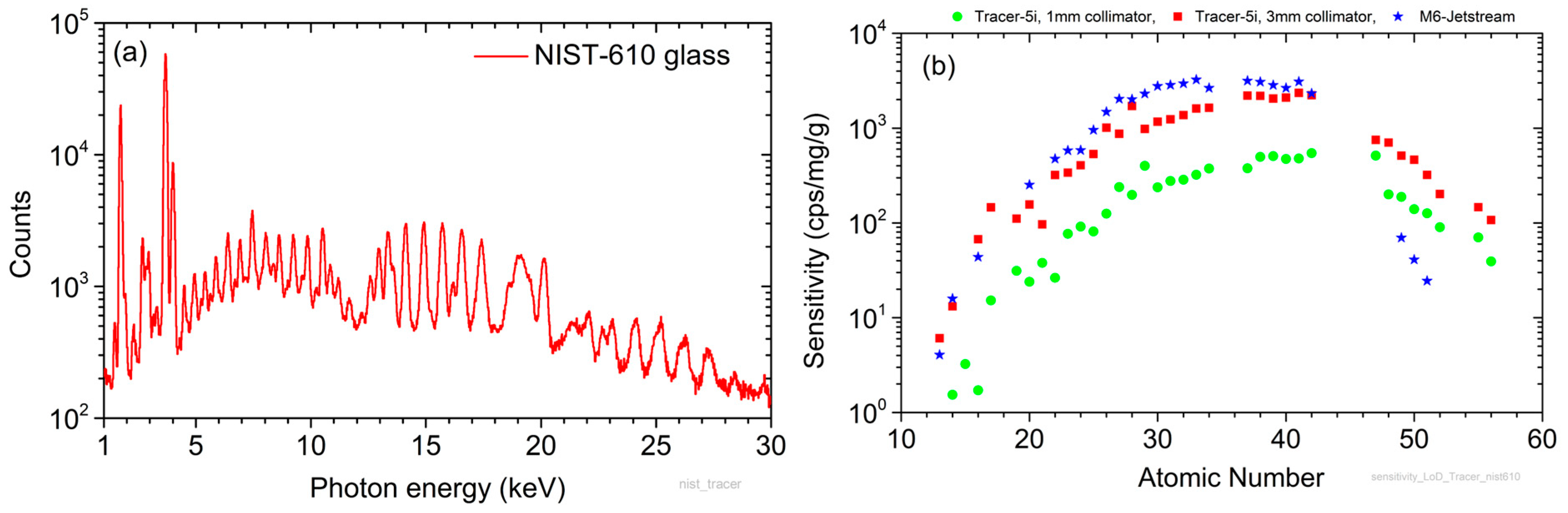
The scanner’s analytical capabilities, such as sensitivity, energy resolution, beam spot size, and intensity variation as a function of the distance between the spectrometer and the target, are assessed. The sensitivity expresses the efficiency of the XRF spectrometer in exciting different elements through the periodic table. The detector’s energy resolution as a function of the measured photon energy is required to define the energy windows for the real-time intensity determination of characteristics transitions using the ROI method. The scanner’s spatial resolution is determined by the beam spot size in combination with the step size. Finally, the knowledge of the intensity variation of the characteristic transition energy as a function of the target’s distance from the spectrometer is imperative for the quantitative analysis.

3.1. Sensitivity

The elemental sensitivity was determined by measuring the Standard Reference Material (SRM) 610 Trace elements in the National Institute of Standards and Technology (NIST) glass. NIST SRM 610 is a 1 mm thick glass disk, containing a broad range of trace elements at a nominal concentration level of 500 ppm [16]. Specifically, sixty-one trace elements are contained in the glass support matrix with a nominal composition of 72% SiO₂, 14% Na₂O, 12% CaO, and 2% Al₂O₃ (mass fractions).

The measurement conditions were high voltage of 50 kV, current of 35 μA, and measuring real time of 120 s. The live time in the case of the 3 mm collimator was 87 s, while in the case of 1 mm it was 106 s. The measured XRF spectrum in the case of a 1 mm collimator is shown in Figure 2a. From the extracted intensities, the sensitivity $S_i$ for element i was calculated by means of Equation (1):

$$S_i={\displaystyle \frac{N_i}{C_i·t_l}}$$

(1)

where $N_i$ is the net intensity of the XRF transition line of element i, $C_i$ is the concentration of element i in the standard, and $t_l$ is the live time of the measurement. Figure 2b shows the extracted sensitivities for the Kα transitions as a function of the atomic number. The sensitivity reaches its maximum values for elements with atomic numbers between Mn (Z = 25) and Mo (Z = 42). For comparison, the extracted sensitivity of Bruker’s state-of-the-art M6-Jetstream scanner is displayed by measuring the NIST SRM 610 with a beam spot of 100 μm and a maximum power of 30 W (50 kV, 600 μA). The sensitivity of M6 decreases significantly at high energies because of the use of a polycapillary lens.

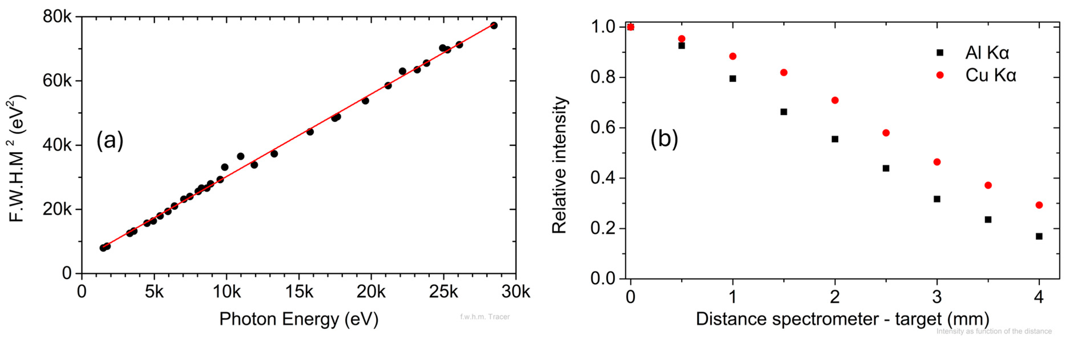
3.2. Energy Resolution

The spectrometer’s energy resolution was determined by fitting the K X-ray characteristic transitions of the XRF spectra emitted from bulk targets using PyMca [17]. The K X-ray characteristic transitions of 32 elements were measured, ranging from aluminum (Z = 13) to tin (Z = 50). The full width at half maximum (FWHM) of the Gaussian distributions, in electronvolt (eV), describing the measured line shape of the recorded characteristic transitions as a function of the photon energy $E_{ph}$ (eV), is given by Equation (2), and it is shown in Figure 3a:

$$FWHM\left(eV\right)=\sqrt{2.57\left(3\right)·E_{ph}\left(eV\right)+4.5\left(4\right)·{10}^3}$$

(2)

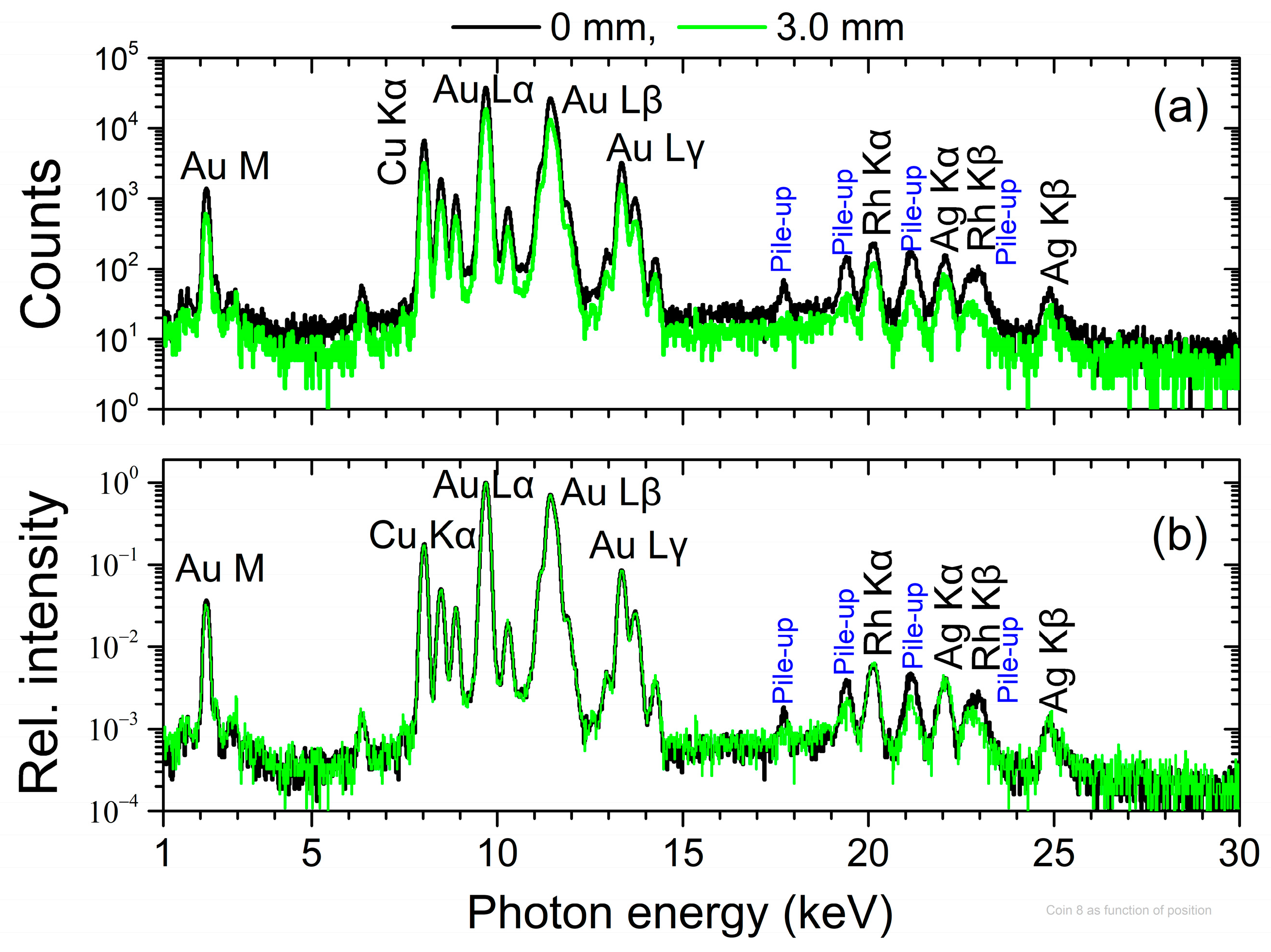
3.3. Intensity as a Function of the Distance

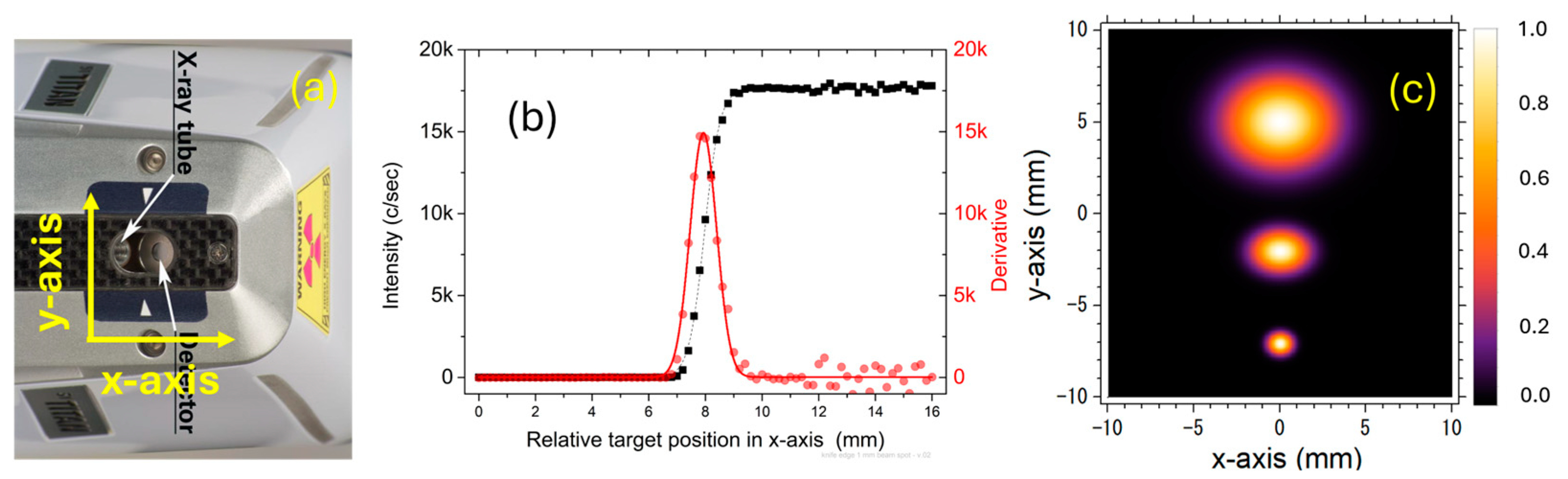
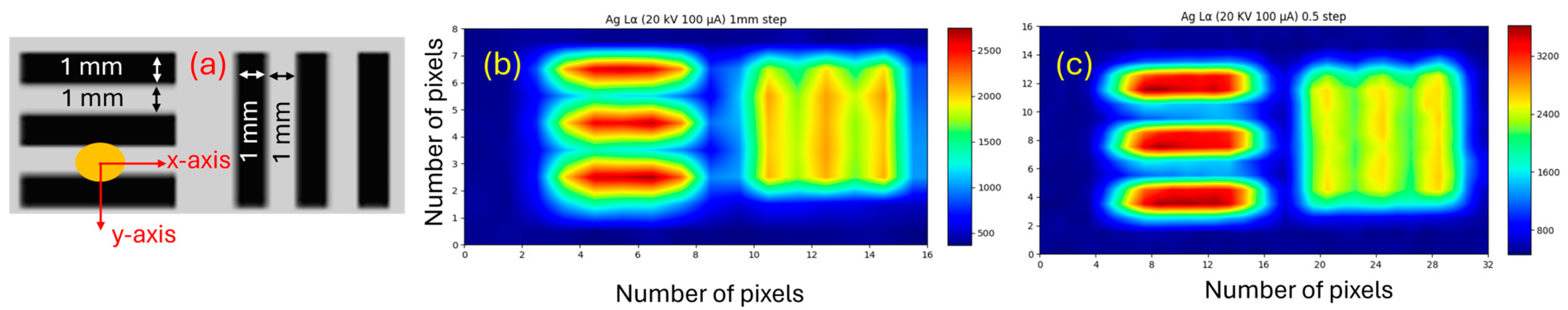
Using the handheld in scanning mode, the target must not be in contact with the spectrometer’s head. Moreover, the distance in between may vary due to a non-flat target or to the different heights of multiple targets. The measured intensities decrease as the distance increases due to the reduction in detection solid angle and photon absorption in the air. Solid angle reduction is a geometric factor that is identical for all transitions, independent of the photon’s energy. Instead, the photon absorption in air is a function of the photon’s energy. In Figure 3b, the measured intensities of the Al Κα and Cu Kα transitions as a function of the spectrometer-target distance are displayed. The decrease in Cu Kα intensity as a function of distance primarily reflects the reduction in solid angle, as the mean attenuation length of 8 keV photons (Cu Kα) in the air is about 85 mm [18]. The decrease in Al Kα intensity as a function of distance, except the reduction in solid angle, involves the photon absorption in the air path, as the mean attenuation length of 1.49 keV photons (Al Kα) in the air is about 7 mm [18]. Additionally, matrix effects may also contribute to a lesser extent due to the variation of incoming and outgoing angles of photons.

3.4. Beam Spot Size

The beam spot and step size determine the scanner’s spatial resolution. The beam spot on the spectrometer’s measuring plane has an elliptical shape, as the ionization beam impinges on it not vertically but at an angle of about 45° (Figure 4a). The beam spot size was determined by scanning a pure copper bulk target using the knife-edge method [19], both across the long axis (defined as the x-axis) and the short axis (defined as the y-axis). In Figure 4b, the measured intensities of Cu Kα are shown along the x-axis of the beam for a distance between the spectrometer’s measuring plane and the target’s surface of 0.3 mm. As illustrated in Figure 4b, the beam spot distribution is estimated by calculating the full width at half maximum (FWHM) of a Gaussian distribution fitted to the derivative of the spectral distribution. The FWHM values were extracted for all three collimators, in both long and short sides, for distances of 0.3, 0.6, 1.0, 1.5, and 2.0 mm. The beam spot size for the distance sample-spectrometer up to 2.0 mm was found to be unchanged, which should be attributed to the collimator’s cylindrical shape.

Table 1. Gaussian widths of the beam spot distribution along the short and long sides for each collimator.

Collimator	Beam Spot FWHM (mm)		Beam Spot FWTM (mm)
	x-axis	y-axis	x-axis	y-axis
“1 mm”	1.1 ± 0.1	0.9 ± 0.1	2.0 ± 0.2	1.6 ± 0.2
“3 mm”	2.5 ± 0.1	1.70 ± 0.05	4.6 ± 0.2	3.1 ± 0.1
“8 mm”	4.9 ± 0.1	3.75 ± 0.05	8.9 ± 0.2	6.8 ± 0.1

shows the extracted FWHM values and the evaluated FWTM (the full-width tenth maximum (FWTM) is defined as the width of the Gaussian distribution at a level that is 1/10 the maximum ordinate of the peak) for each collimator during the scanning in the x- and y-axis. The calculated two-dimensional beam spot profile for each of the three collimators is given in Figure 4c. The two-dimensional profile was modeled by the product of two Gaussians, one along the x-axis and the other along the y-axis, with the FWHM values given in Table 1. Each Gaussian was assigned a peak intensity equal to one unit.

The effect of the scan step on the spatial resolution was studied by scanning the structure of a silver-printed USAF1951 resolution test target [20]. A two-dimensional scan was performed on the structure with group number {−1} and element number {1} [21]. This structure, shown in Figure 5a has line thicknesses and spacings of 1 mm. The intensity distribution map for Ag Lα with a 1 mm collimator is shown in Figure 5b for a 1.0 mm scan step and in Figure 5c for a 0.5 mm scan step.

4. Measurements and Discussion

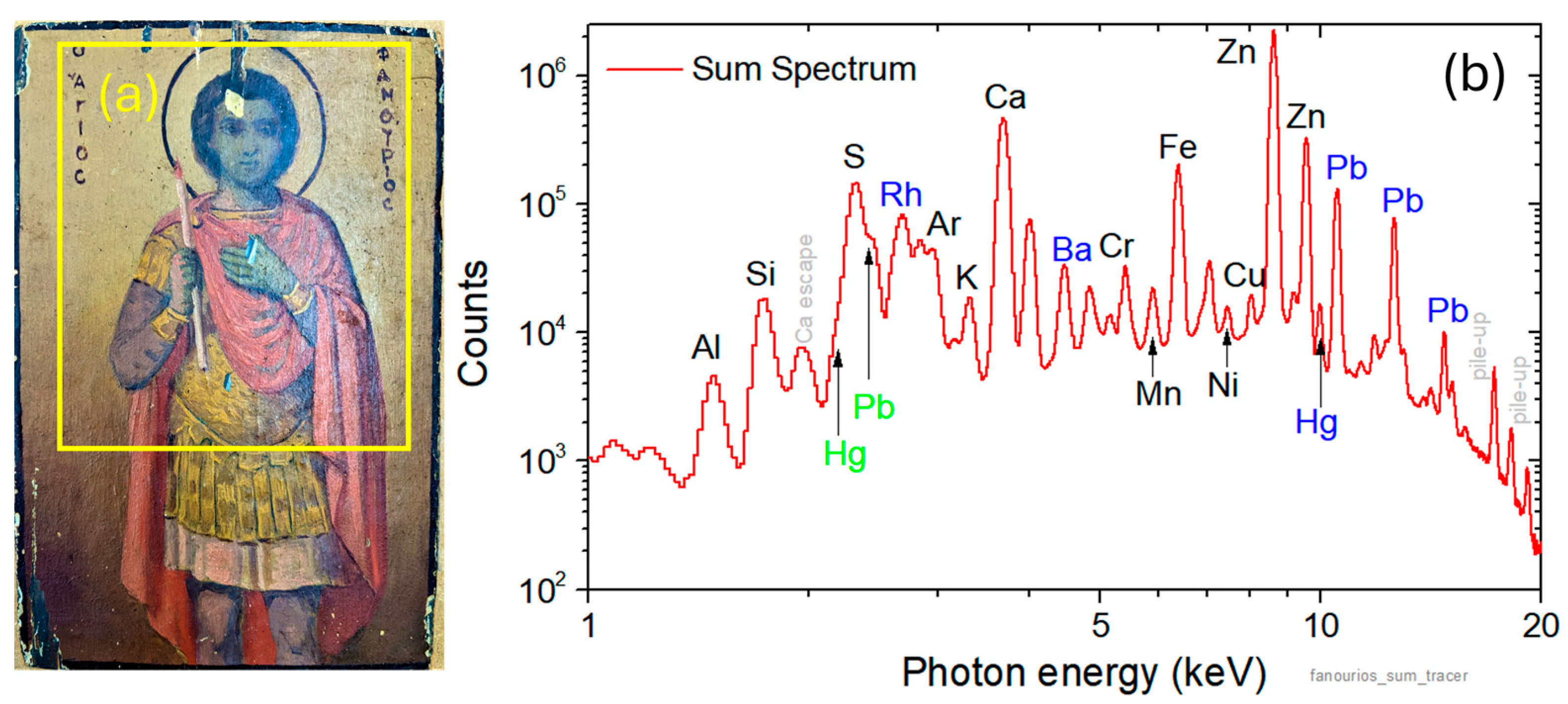
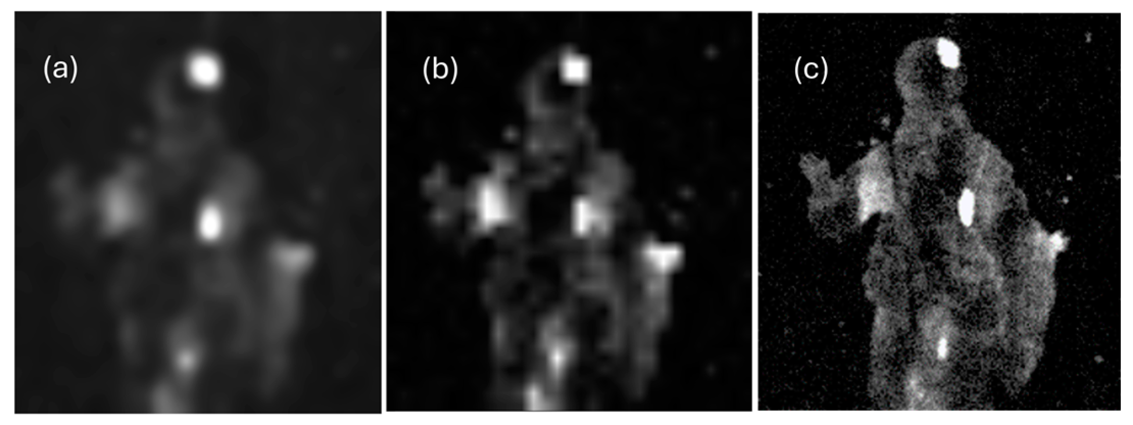
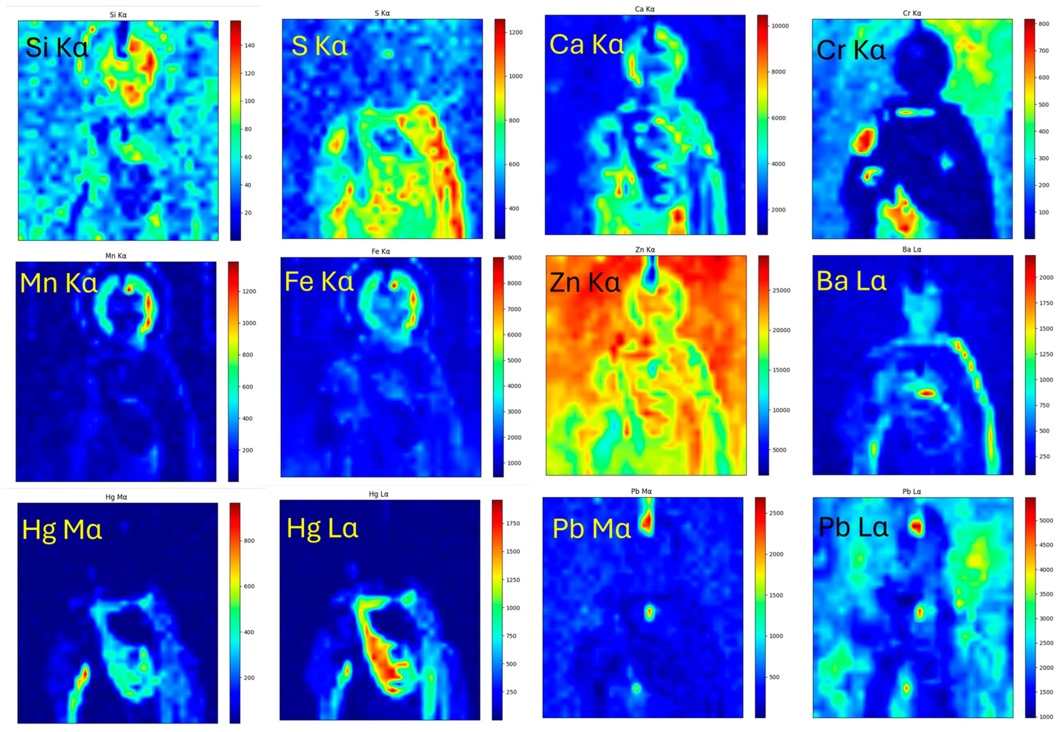
4.1. Imaging

The XRF scanner imaging capabilities are being tested by studying a Greek religious panel painting (“icon”). In particular, an area measuring 10 × 9 cm² on a small, late 19th-century panel painting that depicts St. Fanourios (from the Greek word “fanerono”, i.e., “reveal”) shown in Figure 6a was scanned. Note that the scanned area is considered representative of the whole painting, as it includes all the different colors and tonalities. The measuring conditions were a high voltage of 20 kV, a current of 20 μA, a 3 mm collimator, a step of 3 mm, and no beam filter. The studied area was scanned point by point, with the minimum feasible measuring time of 1 s. This results in approximately 600 spectra per hour, considering that about 4–5 s are required for the spectrometer to be ready for the next measurement. In total, 1054 (34 × 31) spectra were collected, and the overall measuring time was 1.3 h. Figure 6b shows the sum spectrum upon completion of scanning. The spectra analysis revealed the presence of the elements aluminum (Al), silicon (Si), sulfur (S), potassium (K), calcium (Ca), chromium (Cr), manganese (Mn), iron (Fe), copper (Cu), zinc (Zn), mercury (Hg), lead (Pb) and barium (Ba).

The ability to convert binary files to ASCII allows the spectrometer’s recorded parameters to be monitored in real-time. For example, the dead-time value per pixel is displayed in Figure 7a, taking values in the range of 4–10%. Figure 7b displays the spectrometer’s ambient air temperature as a function of the measured pixel and equivalently to the measuring time. The spectrometer’s ambient air temperature rose from 30 °C at the beginning of the measurement to 40 °C with the completion of the measurement. The detector’s temperature was found to stay constant at −27 °C during the 1.3 h of measurement.

The elemental distribution maps can be generated either online in real time using the ROI method or offline using PyMca code (version 5.6.7) [17]. The ROI window is centered on the selected energy peak, and its width is determined by the FWHM value according to Equation (2), scaled by a user-defined factor. A comparison of the two approaches is demonstrated in Figure 8, where pertinent examples of the elemental distribution maps of copper (Cu) are shown, which clearly reveal the presence of an older painting that lies beneath the representation of St Fanourios. Figure 8a corresponds to the Cu-distribution map created online using the ROI method, whereas Figure 8b shows the Cu map created offline using PyMca; it is apparent that both methods lead to comparable results, and the real-time analysis is more than acceptable. Nevertheless, thanks to the fitting procedure, the PyMca map is evidently less noisy, as it reveals subtle differences in details. To confirm the Cu elemental map’s accuracy, we compared it to the Cu distribution obtained by scanning the icon using M6-Jetsream shown in Figure 8c. For the measurement, the X-ray tube was operated at a high voltage of 50 kV and a current of 600 μA. No absorption filter was applied on the beam path of the ionization radiation. The pixel size was 500 × 500 μm², and the dwell time was 25 ms per pixel. The spot size was set at 580 μm (Mo Κα). Apart from the exceptional spatial resolution provided by M6-Jetstream due to its significantly smaller beam spot, the image form is fully reproduced. Here, it is worth mentioning that, as veneration objects, icons were occasionally partially or completely overpainted (i.e., covered by new paint layers) in the framework of past restoration/renovation treatments, and this practice has been documented before [22,23].

Although the ROI method is easy to apply in real-time analysis, it may prove problematic in the case of energy overlap of spectral lines, such as the S Κα and Pb Mα transitions. Therefore, the acquired XRF spectra are fitted offline using PyMCA [17], and the obtained elemental maps are shown in Figure 9.

Based on the assessment of the detected elements’ distribution and the corresponding areas’ color, certain conclusions regarding the employed painting materials/pigments and techniques were extracted. In particular, the distribution of Fe indicates the use of an ochre-type pigment on areas like the flesh and the shadowy parts of the vestments, while the strong correlation of Fe with Mn in the dark brown pictorial elements like the hair, the halo outline, and the inscriptions clearly hints towards the employment of Mn-rich iron earth—i.e., an umber—in these very areas [24]. The presence of Si appears to correlate with Fe, too, and this may well pertain to the presence of natural Fe-bearing ochre, which is known to contain (clayey) substances rich in silicon [25]. Detection of Hg obviously pertains to the use of vermilion (HgS); therefore, it is not surprising that it was exclusively detected on St Fanourios’ red vestment and the candle flame. Contrarily, the yellow areas—the armor and the bracelets—show predominantly Cr, implying thus the use of chrome yellow [26]. The off-white and bright areas (e.g., candle, flesh, background, and vestment highlights) appear dominated by Zn, an element that indicates the employment of zinc oxide. The latter corresponds to a synthetic white pigment that became particularly widespread after the mid-19th century [26], and its detection is consistent with the dating of the painting in consideration. Additionally, the elements S, Ca, and Ba pertain primarily to color additives/fillers, like calcium sulfate/carbonate and barium sulfate compounds, often added in commercial pigments [27]. It is interesting to note that lead is also detected due to its presence in the subject paint layers, as its major intensity areas coincide with losses of the upper paint layers (Figure 9). The fact that Pb exists only on the older (subject) painting is corroborated by the distribution map of the Pb Mα transition, which is of significantly lower energy than the Pb Lα (2.34 and 10.55 keV, respectively) and appears only in the areas where losses on the St Fanourios painting are seen. Note that this is not the case for Hg, which is detected due to the employment of a pertinent pigment in the St Fanourios red cloak and, hence, the distribution of Hg Mα and Lα transitions practically coincide (Figure 9).

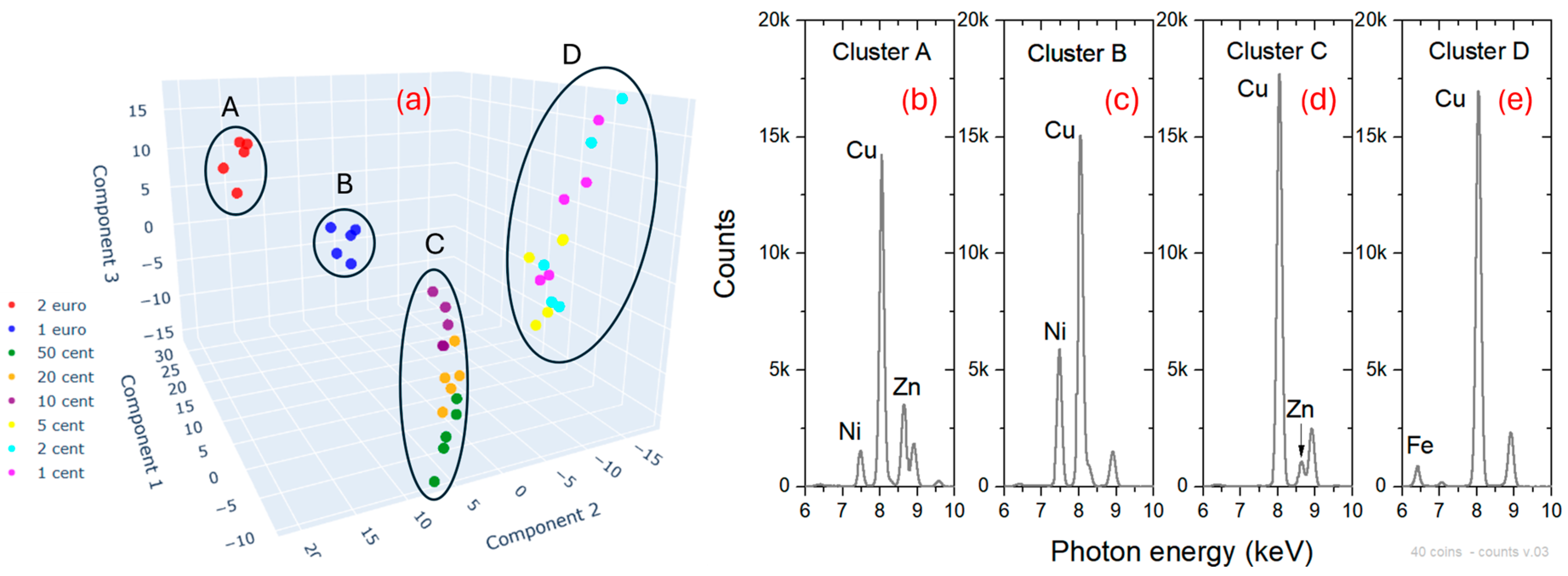
4.2. Object Classification

The study aims to explore the capability of object classification according to their elemental composition by analyzing the acquired raw spectra using dimensionality reduction methods. The goal is to achieve object classification without the user performing any spectroscopic analysis. In the realm of archaeometallurgy, the classification and quantitative analysis of metallic objects are essential.

As a case study, a collection of 40 coins was analyzed [28]. Specifically, five coins of each coin type (1, 2, 5, 10, 20, 50 cents, EUR 1 and 2) were selected. Coins were arranged in a grid pattern on a polymer holder using circular excavated mountings. The distance between successive mounts is 20 mm, while the diameter of each mount is 10 mm, and its depth is 1.7 mm. The distance between the spectrometer’s head and the top of the sample holder was set at about 1 mm. The tube’s high voltage was set at 30 kV, the current at 5 μA, the 3 mm collimator was used, and no beam filter was applied. The measurement time per coin was set to 1 s. All the coins were irradiated at their center, which means that the 1 and 2-euro coins were irradiated at their inner disk.

The measured spectra were transmitted wirelessly to the analysis workstation in real time through the network. Simultaneously, the data files are decoded from the “pdz” binary form to ASCII format. The 40 spectra were analyzed using Principal Components Analysis (PCA) in linear covariance mode [29]. PCA application allows for reducing the dimensionality of large datasets. The information contained in the spectrum, consisting of 2048 channels, is condensed to a point in three dimensions. A principal component analysis scatterplot based on the three principal components is displayed in Figure 10a (see Supplementary Materials for an interactive HTML 3-D scatter plot web page). Four distinct clusters are observed.

Cluster “A” consists of the 2-euro coins. The mean spectrum of the coins contained in the cluster is shown in Figure 10b. The detected Cu, Ni, and Zn K transitions originate from the coins’ inner disk, which has a nominal weight percentage composition of 75% Cu, 5% Ni, and 20% Zn [30]. Cluster “Β” consists of the 1-euro coins. The mean spectrum of the coins contained in the cluster is shown in Figure 10c. The detected Cu and Ni K transitions originate from the coins’ inner disk, which has a nominal weight percentage composition of 75% Cu and 25% Ni [30].

Cluster “C” consists of fifteen coins, including the 10-, 20-, and 50-cent coins. All these coins have a nominal weight percentage elemental composition of 89% copper, 5% zinc, 5% aluminum, and 1% tin [30]. The mean spectrum of the coins contained in the cluster, in the energy region 6–10 keV, is shown in Figure 10d. As can be deduced from Figure 10a, these coins are grouped into three subclusters, each containing the 10-cent, 20-cent, and 50-cent coins. The 20-cent coins are in between the other two subclusters. Although the nominal elemental composition of all these coins is identical, the intensities of Cu and Zn, as can be seen in Figure 11a, increase as a function of the coin’s nominal value. This should be attributed to the thickness of the coins, which is 2.38 mm for the 50-cent coin, 2.14 mm for the 20-cent coin, and 1.93 mm for the 10-cent coin [31]. The distance between the spectrometer’s measuring plane and the surface of the coins depends on their value. The 50-cent coin is the closest, while the 10-cent coin is the farthest.

Cluster “D” consists of fifteen coins and includes all the 1-, 2-, and 5-cent coins (Figure 10a). The cluster size is extended, and the distribution of the various coins is random. The coins are composed of a steel substrate with a copper layer on top [30]. The coins have the same nominal thickness of 1.67 mm [31]. The mean spectrum of cluster “D” is shown in Figure 10e. Cu K transitions originate from the layer, while the Fe K transitions originate from the substrate. The widespread scatter of the points in the cluster indicates a variation in the thickness of the copper layer. The thickness variation is inherent across the surface of each of these coins, as confirmed by a line scan across the surface of the 1-cent coin using the XRF scanner. In Figure 11b, the Fe Κα transition intensity across a diameter of the 1-cent coin is shown. The Fe Κα counts variation indicates variations in the thickness of the copper layer, with the smallest Cu layer thickness at the center of the coin [32]. The X-ray tube was operated at 30 kV and 50 μA during the measurement. The measuring time was 3 s, using the homemade collimator of 1 mm with a scan step of 0.5 mm.

The present study demonstrates the strength of object classification in scanning mode based on the raw XRF spectra.

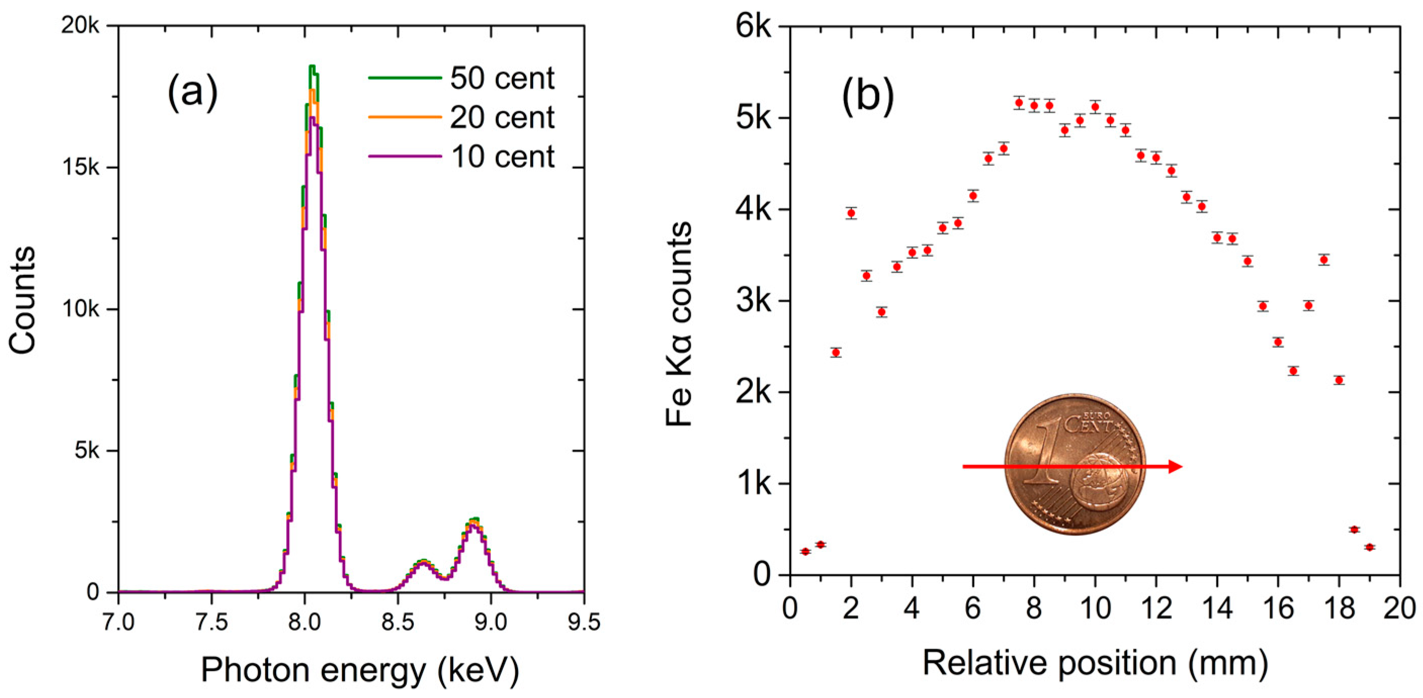
4.3. Quantitative Analysis during Scanning

The XRF scanner’s capability to conduct quantitative analysis during scanning is explored. Using the handheld in scanning mode, the target is not in contact with the spectrometer’s measuring plane. Variation in the distance between the spectrometer’s measuring plane and the target changes the spectrometer’s geometry, including radiation beam incoming and outgoing angles, the detector’s solid angle, and the beam’s air path length. For reliable quantitative analysis, the tolerance to the target–spectrometer distance variation is worth examining.

For this purpose, Au–Ag–Cu bulk alloy targets were studied due to their fundamental importance in cultural heritage. The elemental composition of eight alloys was determined by XRF positioning them one by one on the spectrometer’s measuring plane (distance “0 mm”). The measuring conditions were high-voltage 40 kV, current 7 μA, measuring time 15 s, and using the Ti/Al filter. The “Precious metals” routine installed on the handheld Bruker’s Tracer-5i was applied to determine the alloy’s elemental concentration. The intensities of the Cu Kα (8.05 keV), Au Lα (9.71 keV), and Ag Kα (22.2 keV) transitions are used for the quantification.

Table 2. Elemental weight concentration for the eight alloys according to the pre-installed “Precious metals” routine. The numbers in parentheses correspond to the two standard deviation values.

Distance	Element	Alloy 1	Alloy 2	Alloy 3	Alloy 4	Alloy 5	Alloy 6	Alloy 7	Alloy 8
“0 mm”	Cu	7.4 (1)	47.2 (2)	47.4 (2)	8.7 (1)	27.4 (1)	10.0 (1)	8.1 (1)	8.2 (1)
	Zn	—	—	6.2 (1)	—	6.8 (1)	—	—	—
	Ag	92.6 (3)	20.8 (2)	7.0 (1)	29.1 (2)	8.3 (1)	0.35 (5)	0.39 (5)	0.82 (5)
	Au	—	31.9 (2)	39.3 (2)	61.9 (3)	57.5 (3)	89.6 (3)	91.5 (1)	91.0 (1)
“3 mm”	Cu	7.5(1)	47.1 (2)	47.4 (2)	8.9 (1)	27.3 (2)	10.0 (1)	8.3 (1)	8.2 (1)
	Zn	—	—	5.6 (1)	—	6.4 (1)	—	—	—
	Ag	92.5 (4)	21.2 (2)	7.3 (1)	29.7 (3)	8.5 (2)	0.35 (7)	0.45 (5)	0.94 (6)
	Au	—	31.7 (2)	39.7 (3)	61.4 (3)	57.8 (4)	89.6 (4)	91.2 (1)	90.8 (1)

gives the eight alloys’ extracted weight concentrations of gold, copper, silver, and zinc. The concentration percentages of gold and silver cover a broad weight percentage range.

The eight alloys were re-measured successively in scanning mode, with the distance of the spectrometer’s measuring plane to the coins’ surface set at about 3 mm (distance “3 mm”). The measuring conditions remained unchanged. The elemental weight concentrations for each target are extracted by applying the “Precious metals” routine. The weight concentrations of gold, copper, silver, and zinc for the distance “3 mm” are given in Table 2. The concentrations extracted are in excellent agreement, within the error bars, to those obtained by measuring each coin on the distance “0 mm”.

To interpret the achieved precision on the quantitative analysis, we studied the measured XRF spectra of alloy 8” at the two measurement distances of “0 mm” and “3 mm”. The measured spectra are displayed in Figure 12a. As can be deduced, the absolute intensities are reduced significantly at the “3 mm” distance relative to “0 mm”. In Figure 12b, the two spectra were normalized to the Au Lα intensity. The two spectra display excellent agreement for the relative intensities of the Cu K, Au L, and Ag K transitions, indicating that they only differ by a proportionality factor. The proportionality factor, independent of photon energy, results from the change in the detection solid angle. The energy-dependent photon absorption in the air is negligible due to the small variation in the beam path compared to the mean attenuation length of these high-energy characteristic transitions. In addition, it is deduced that the matrix effect is insignificant. Observing the normalized spectra, the pile-up peaks are not in coincidence. This is because the pile-up intensities are proportional to the square of the involved transition intensities.

The present study demonstrates that quantitative analysis in scanning mode is feasible, provided that the permissible tolerances at the distance of the spectrometer’s head from the target are thoroughly investigated.

5. Conclusions

An X-ray fluorescence scanner was developed by coupling the Bruker Tracer 5i XRF handheld spectrometer with a low-cost automated x–y motion control system. A Python-based control program offers an intuitive interface for operating the scanner and enabling handheld remote control. The measured spectra are swiftly transmitted over the Internet to the analyzing workstation, where they are promptly decoded into ASCII format, stored, and analyzed in real time. This real-time analysis capability significantly enhances the system’s efficiency, allowing for immediate insights and adjustments.

The XRF scanner’s performance was thoroughly evaluated, considering its characteristics such as sensitivity, energy resolution, beam spot size, and intensity variation. This comprehensive evaluation provides a clear understanding of the scanner’s capabilities and limitations.

Three case studies illustrate the scanner’s efficiency and functionality for imaging, object classification, and quantitative analysis, demonstrating its notable performance. The imaging capabilities of the XRF scanner were tested by studying a religious icon. The icon was scanned point by point, with an acquisition rate of about 600 spectra per hour. In total, 1054 XRF spectra were recorded. Elemental maps were extracted either in real-time, using the ROI method, or offline by fitting the spectra using PyMca. Based on assessing the detected elements’ distribution, conclusions were extracted regarding the employed painting materials/pigments and techniques. The accuracy of the extracted maps was validated by comparing them with high-resolution maps obtained from the M6-Jetstream. The scanning mode of Tracer-5i is noticeably slower, not due to its sensitivity but to the necessary time per measured point. Moreover, its spatial resolution is inferior to a polycapillary optic scanner. However, the portability and low acquisition cost of the Tracer-5i make it an appealing alternative for XRF scanning.

The scanner’s ability to classify objects is demonstrated by measuring a set of all the types of euro coins in scanning mode. The coins are automatically categorized into distinct clusters based on their composition through real-time evaluation of the raw spectra using PCA analysis.

Finally, the scanner’s ability for quantitative analysis in real time is demonstrated by studying a set of precious alloys containing gold, silver, and copper. The Tracer-5i “Precious metals” routine by Bruker was used to determine the alloys’ elemental concentration, both in touch with the spectrometer’s head and in scanning mode. The extracted elemental weight concentrations are in perfect agreement. It is important to note that the precision achieved by scanning elemental analysis is only reliable when the intensity of the spectral lines used for quantitative analysis decreases at the same rate as a function of the target’s distance from the spectrometer’s head.

In conclusion, we have successfully adapted the Tracer-5i with a low-cost, controllable x–y table for real-time imaging, object classification, and quantitative elemental analysis in scanning mode. This achievement allows the implementation of the next stage, which involves scanning with the spectrometer towards a fixed target.

References

1. Alfeld, M.; Pedroso, J.V.; van Eikema Hommes, M.; Van der Snickt, G.; Tauber, G.; Blaas, J.; Haschke, M.; Erler, K.; Dik, J.; Janssens, K. A Mobile Instrument for in Situ Scanning Macro-XRF Investigation of Historical Paintings. J. Anal. At. Spectrom. 2013, 28, 760–767. [Google Scholar] [CrossRef]
2. Romano, F.P.; Caliri, C.; Nicotra, P.; Di Martino, S.; Pappalardo, L.; Rizzo, F.; Santos, H.C. Real-Time Elemental Imaging of Large Dimension Paintings with a Novel Mobile Macro X-ray Fluorescence (MA-XRF) Scanning Technique. J. Anal. At. Spectrom. 2017, 32, 773–781. [Google Scholar] [CrossRef]
3. Mastrotheodoros, G.P.; Asvestas, A.; Gerodimos, T.; Anagnostopoulos, D.F. Revealing the Materials, Painting Techniques, and State of Preservation of a Heavily Altered Early 19th Century Greek Icon through MA-XRF. Heritage 2023, 6, 1903–1920. [Google Scholar] [CrossRef]
4. Mastrotheodoros, G.P.; Asvestas, A.; Gerodimos, T.; Tzima, A.; Papadopoulou, V.; Anagnostopoulos, D.F. MA-XRF Investigation of a 17th Century Icon by the Renowned Painter Theodoros Poulakis. J. Archaeol. Sci. Rep. 2024, 53, 104313. [Google Scholar] [CrossRef]
5. Shugar, A.N.; Mass, J.L. Handheld XRF for Art and Archaeology; Leuven University Press: Leuven, Belgium, 2012; ISBN 978-90-5867-934-5. [Google Scholar]
6. Clarke, M.L.; Gabrieli, F.; Rowberg, K.L.; Hare, A.; Ueda, J.; McCarthy, B.; Delaney, J.K. Imaging Spectroscopies to Characterize a 13th Century Japanese Handscroll, The Miraculous Interventions of Jizō Bosatsu. Herit. Sci. 2021, 9, 20. [Google Scholar] [CrossRef]
7. Shugar, A.N. Handheld Macro-XRF Scanning: Development of Collimators for Sub-mm Resolution. In Proceedings of the Fourth International Symposium on Analytical Methods in Philately, Washington, DC, USA, 13–14 November 2020; pp. 13–20. [Google Scholar]
8. Shugar, A.N.; Drake, B.L.; Kelley, G. Rapid Identification of Wood Species Using XRF and Neural Network Machine Learning. Sci. Rep. 2021, 11, 17533. [Google Scholar] [CrossRef] [PubMed]
9. Hoffmann, P.; Flege, S.; Ensinger, W.; Wolf, F.; Weber, C.; Seeberg, S.; Sander, J.; Schultz, J.; Krekel, C.; Tagle, R.; et al. MA-XRF Investigation of the Altenberg Retable from 1330. X-ray Spectrom. 2018, 47, 215–222. [Google Scholar] [CrossRef]
10. Handheld XRF Spectrometers TRACER 5. Available online: https://www.bruker.com/en/products-and-solutions/elemental-analyzers/handheld-xrf-spectrometers/TRACER-5.html (accessed on 10 May 2024).
11. G-Code. Available online: https://en.wikipedia.org/wiki/G-code (accessed on 16 April 2024).
12. Available online: https://github.com/pywinauto/pywinauto (accessed on 16 April 2024).
13. ESP32 Series of Modules. Available online: https://www.espressif.com/en/products/modules/esp32 (accessed on 16 April 2024).
14. FluidNC. Available online: https://github.com/bdring/FluidNC (accessed on 16 April 2024).
15. wget 3.2. Available online: https://pypi.org/project/wget/#description (accessed on 30 April 2024).
16. Standard Reference Material® 610. Available online: https://tsapps.nist.gov/srmext/certificates/610.pdf (accessed on 16 April 2024).
17. Solé, V.A.; Papillon, E.; Cotte, M.; Walter, P.; Susini, J. A Multiplatform Code for the Analysis of Energy-Dispersive X-ray Fluorescence Spectra. Spectrochim. Acta Part B At. Spectrosc. 2007, 62, 63–68. [Google Scholar] [CrossRef]
18. X-ray Interactions with Matter. Available online: https://henke.lbl.gov/optical_constants/gastrn2.html (accessed on 30 April 2024).
19. Sitko, R.; Zawisza, B.; Malicka, E. Energy-Dispersive X-ray Fluorescence Spectrometer for Analysis of Conventional and Micro-446 Samples: Preliminary Assessment. Spectrochim. Acta Part B At. Spectrosc. 2009, 64, 436–441. [Google Scholar] [CrossRef]
20. Gerodimos, T.; Patakiouta, I.V.; Papadakis, V.M.; Exarchos, D.; Asvestas, A.; Kenanakis, G.; Matikas, T.E.; Anagnostopoulos, D.F. Scanning Micro X-ray Fluorescence and Multispectral Imaging Fusion: A Case Study on Postage Stamps. J. Imaging 2024, 10, 95. [Google Scholar] [CrossRef] [PubMed]
21. 1951 USAF Resolution Test Chart. Available online: https://en.wikipedia.org/wiki/1951_USAF_resolution_test_chart (accessed on 3 May 2024).
22. Daniilia, S.; Bikiaris, D.; Burgio, L.; Gavala, P.; Clark, R.J.H.; Chryssoulakis, Y. An Extensive Non-Destructive and Micro-Spectroscopic Study of Two Post-Byzantine Overpainted Icons of the 16th Century. J. Raman Spectrosc. 2002, 33, 807–814. [Google Scholar] [CrossRef]
23. Cortea, I.M.; Ratoiu, L.; Chelmuș, A.; Mureșan, T. Unveiling the original layers and color palette of 18th century overpainted Transylvanian icons by combined X-ray radiography, hyperspectral imaging, and spectroscopic spot analysis. X-ray Spectrom. 2022, 51, 26–42. [Google Scholar] [CrossRef]
24. Mastrotheodoros, G.P.; Beltsios, K.G. Pigments—Iron-based red, yellow, and brown ochres. Archaeol. Anthropol. Sci. 2022, 14, 35. [Google Scholar] [CrossRef]
25. Helwig, K. Iron oxide pigments: Natural and synthetic. In Artists Pigments: A Handbook of Their History and Characteristics; Berrie, B.H., Ed.; National Gallery of Art: Washington, DC, USA, 2007; Volume 4, pp. 1–37. [Google Scholar]
26. Eastaugh, N.; Walsh, V.; Chaplin, T.; Siddall, R. Pigment Compendium: A Dictionary and Optical Microscopy of Historical Pigments; Butterworth-Heinemann: Oxford, UK, 2008. [Google Scholar]
27. Rogge, C.E.; Epley, B.A. Behind the Bocour Label: Identification of Pigments and Binders in Historic Bocour Oil and Acrylic Paints. J. Am. Inst. Conserv. 2017, 56, 15–42. [Google Scholar] [CrossRef]
28. Shilstein, S.S.; Shalev, S. Making Sense out of Cents: Compositional Variations in European Coins as a Control Model for Archaeometallurgy. J. Archaeol. Sci. 2011, 38, 1690–1698. [Google Scholar] [CrossRef]
29. Abdi, H.; Williams, L.J. Principal component analysis. Wiley Interdiscip. Rev. Comput. Stat. 2010, 2, 433–459. [Google Scholar] [CrossRef]
30. Technical Characteristics of Euro coins. Available online: https://www.bcl.lu/en/Banknotes-and-Coins/billets_pieces/car_pieces/car_tec/index.html (accessed on 28 April 2024).
31. Common Sides of Euro Coins. Available online: https://economy-finance.ec.europa.eu/euro/euro-coins-and-notes/euro-coins/common-sides-euro-coins_en (accessed on 24 April 2024).
32. Electroplating: How the U.S. Mint Makes a Penny. Available online: https://www.comsol.com/blogs/electroplating-u-s-mint-makes-penny/ (accessed on 28 April 2024).
Figure 1. (a) Tracer 5i supported on a tripod, the remote-controlled x–y stage, and the control box. (b) System topology.
Sustainability 16 06135 g001
Figure 2. (a) XRF spectrum of the NIST-610 standard glass. The measurement conditions were 50 kV, 35 μA, real time of 120 s, and 1 mm collimator. (b) Sensitivity for the Kα transition of the elements Z = 13–56, for the 1- and 3-mm collimators. The sensitivity of the M6-Jetstream Bruker scanner is shown for comparison.
Sustainability 16 06135 g002
Figure 3. (a) FWHM as a function of the photon energy. (b) Relative intensity as a function of the distance between the sample’s surface and the spectrometer’s nose. A relative intensity equal to 1 corresponds when the sample is attached to the spectrometer’s nose.
Sustainability 16 06135 g003
Figure 4. (a) Spectrometer’s measuring plane and definition of the x-axis (long side) and the y-axis (short side). (b) Knife edge scan across the x-axis of a Cu pure target for the 1 mm diameter collimator and for a space of 0.3 mm between the spectrometer’s measuring plane and target. The Gaussian distribution fitted to the derivative of the spectral distribution determines the beam spot spreading. (c) Evaluated two-dimensional beam spot profile for each of the three collimators according to the FWHM values in Table 1.
Sustainability 16 06135 g004
Figure 5. (a) Pattern corresponding to group number {−1}, element {1} of the USAF-1951 resolution test chart (see text). (b) Ag Lα intensity distribution for a 1 mm collimator and 1 mm step. (c) Ag Lα intensity distribution for a 1 mm collimator and 0.5 mm step size (oversampling).
Sustainability 16 06135 g005
Figure 6. (a) St. Fanourios, late 19th century. The scanned area is in the yellow rectangle. (b) The sum of the 1054 XRF spectra acquired during the scanning. The energy position of the Kα, Lα, and Mα elemental characteristic transitions are shown in black, blue, and green, respectively.
Sustainability 16 06135 g006
Figure 7. (a) Dead-time value as a function of the measured pixel. (b) Spectrometer’s ambient air temperature as a function of measured pixel (or equivalently to the measuring time). The scan is horizontal line by horizontal line, and the top left pixel is the first measured.
Sustainability 16 06135 g007
Figure 8. Cu elemental distribution map based on the Cu Kα transition: (a) applying real time using the ROI method on the XRF spectra acquired during the scanning with the Tracer-5i, (b) applying offline fitting of the same spectra using PyMca [17], (c) using the M6-Jetstream software (Esprit-M6 v.1.6) on the XRF spectra acquired during the scanning with M6-Jetstream.
Sustainability 16 06135 g008
Figure 9. Εlemental distribution maps applying off-line analysis using PyMca [17].
Sustainability 16 06135 g009
Figure 10. (a) 3-D principal component analysis scatterplot. (be) Mean spectra of each cluster within the 6–10 keV energy.
Sustainability 16 06135 g010
Figure 11. (a) Mean XRF spectra of the 50-cent, 20-cent, and 10-cent coins. (b) Fe Kα transition intensity distribution during linear scan across the diameter of 1-cent coin, revealing the non-uniformity of the copper layer thickness.
Sustainability 16 06135 g011
Figure 12. (a) XRF spectra of alloy “8” for distances of the spectrometer’s measuring plane to the target of 0 mm and 3.0 mm. (b) The XRF spectra normalized to the peak intensity of the Au Lα transition (9.7 keV).
Sustainability 16 06135 g012