
Research on Multi-Objective Optimization of Shield Tunneling Parameters Based on Power Consumption and Efficiency


Abstract
:1. Introduction
2. Parameters
2.1. Power Consumption and Efficiency Calculation Methods
2.2. Data Selection
3. Project Overview
3.1. Section Division
3.2. Tunneling Parameters for Each Section
4. Parameter Optimization
4.1. Optimization Model Selection
4.2. Selection of Multi-Objective Optimization Algorithm
4.3. Optimization Results
5. Discussion
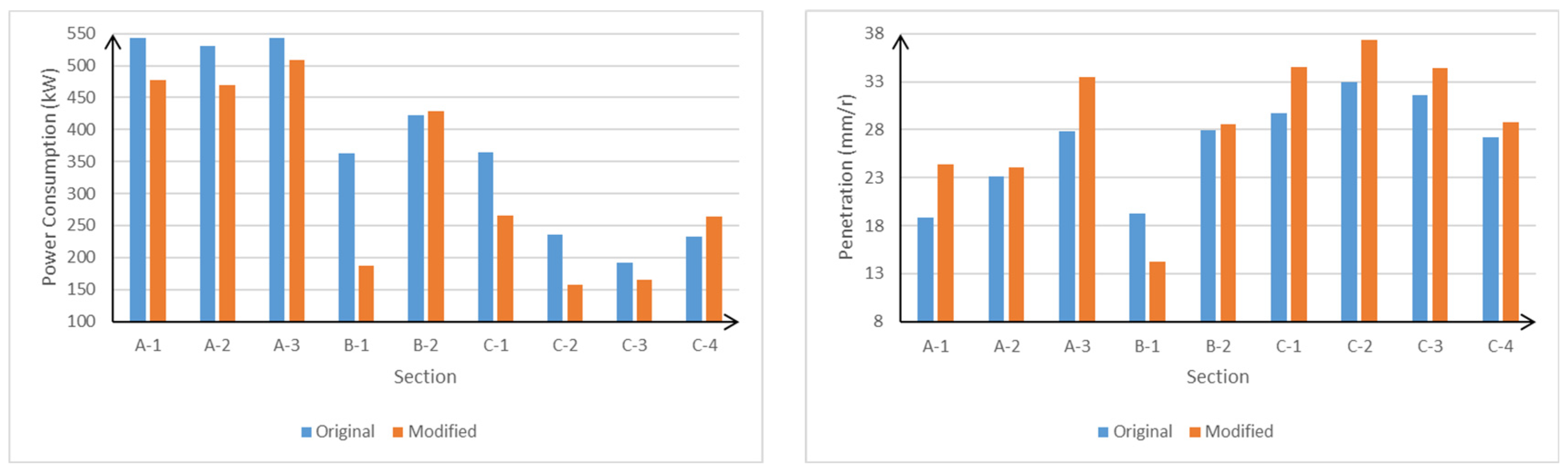
- The multi-objective particle swarm optimization algorithm combined with Pareto optimality principles was used to optimize the tunneling parameters. By employing the weighted sum method (WSM) to select the optimal solution from Pareto solutions, ideal tunneling power consumption and efficiency values under different geological conditions were successfully obtained. After optimization, Section A’s power consumption decreased by approximately 12%, with a 15% increase in efficiency; Section B’s power consumption decreased by about 10%, with an 8% increase in efficiency; and Section C’s power consumption decreased by about 20%, with an 18% increase in efficiency.
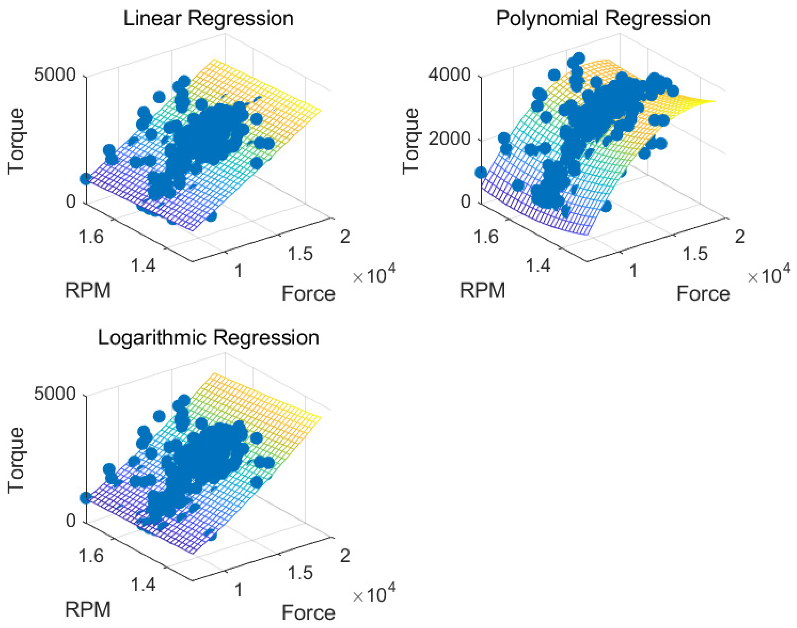
- It was found that cutterhead torque had a higher correlation with thrust and rotational speed, both of which are actively controllable parameters. Therefore, when rapid torque adjustment is needed, prioritizing thrust adjustment can more effectively control power consumption and efficiency.
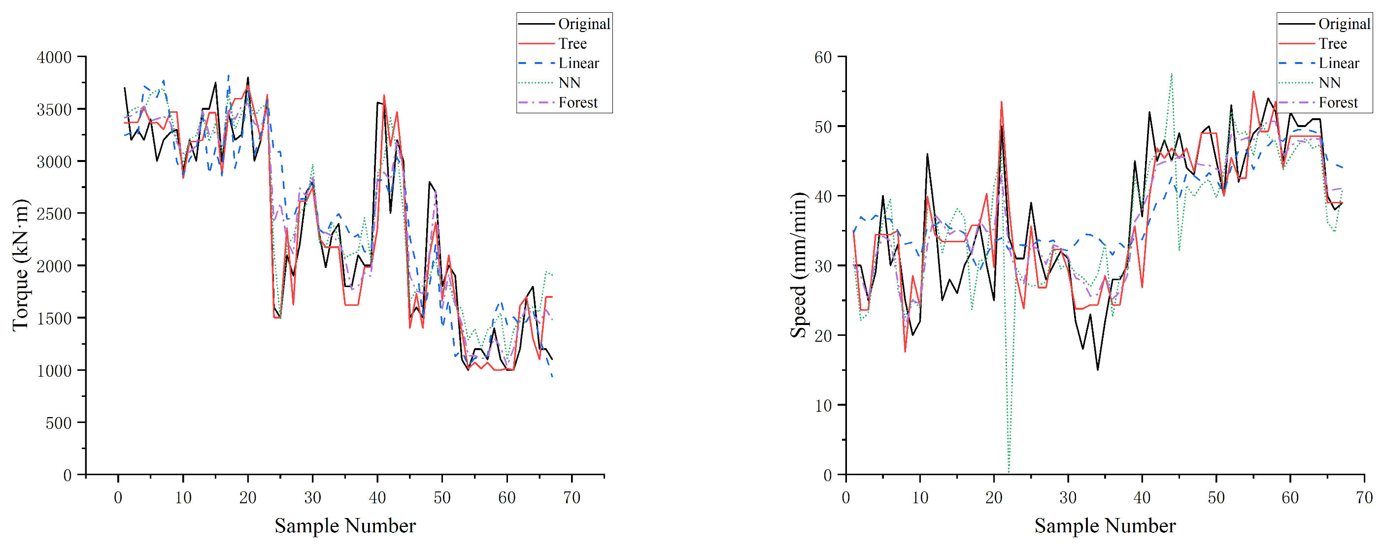
- The parameter values obtained from the Pareto optimal solutions, based on existing data, showed some differences from the predicted values that considered constraints among parameters. These Pareto optimal solutions need to be refined to achieve more accurate evaluations of power consumption and efficiency. Specific adjustment methods include machine learning fitting and re-analysis of parameter relationships.
- In the context of reducing energy consumption and increasing efficiency, the optimized tunneling parameters showed reductions in thrust and cutterhead rotational speed settings. This adjustment strategy is valuable for subsequent projects, providing a significant reference for parameter decision-making in similar projects.
- Expand data collection: Collect a larger scale of shield tunneling data and incorporate different geological parameters to ensure the applicability and stability of the optimization method in various environments.
- Introduce other optimization algorithms: Incorporate other optimization algorithms, such as differential evolution and multi-objective genetic algorithms, and conduct comparative studies to further improve the optimization results.
- Consider more geological parameters: When performing multi-parameter fitting, account for the impact of more geological parameters to improve fitting accuracy. Transform the influence of geological parameters on tunneling conditions into standardized values to quantify the interrelationships among the parameters, thereby enhancing the transferability of the optimization method.
- Conduct more field verifications and adjustments: The optimization results need to undergo more field verification and adjustments. Combine the requirements of project management with factors such as mechanical equipment wear to specifically analyze and dynamically adjust the parameters.
Author Contributions
Funding
Institutional Review Board Statement
Informed Consent Statement
Data Availability Statement
Conflicts of Interest
References
- Li, X.; Wu, J.; Guo, Q.; Xiang, Q.; Geng, F. Calculation model of thrust of shield tunneling based on dimensional theory. Chin. J. Undergr. Space Eng. 2022, 18, 573–577. [Google Scholar]
- Zhang, Y.K.; Gong, G.F.; Yang, H.Y.; Chen, Y.X.; Chen, G.L. Towards autonomous and optimal excavation of shield machine: A deep reinforcement learning-based approach. J. Zhejiang Univ.-Sci. A 2022, 23, 458–479. [Google Scholar] [CrossRef]
- Wu, H.; Chang, J.; Li, G.; Zhang, D.; Huang, H. Prediction of driving posture and optimization of construction parameters for shield based on support vector machine. Tunn. Constr. 2021, 41, 11–18. [Google Scholar]
- Zhang, Z.; Pan, Q.; Zhang, W.; Huang, F. Prediction of surface settlements induced by shield tunnelling using physics-informed neural networks. Eng. Mech. 2024, 41, 1–13. [Google Scholar]
- Men, Y.; Wang, Y.; Zhou, J.; Liao, S.; Zhang, K. Measurement and analysis on EPB shield machine tunneling efficiency in Jinan composite stratum. China Civ. Eng. J. 2019, 52, 110–119. [Google Scholar]
- Lee, H.L.; Song, K.I.; Qi, C.; Kim, J.S.; Kim, K.S. Real-time prediction of operating parameter of TBM during tunneling. Appl. Sci. 2021, 11, 2967. [Google Scholar] [CrossRef]
- Cardu, M.; Catanzaro, E.; Farinetti, A.; Martinelli, D.; Todaro, C. Performance analysis of tunnel boring machines for rock excavation. Appl. Sci. 2021, 11, 2794. [Google Scholar] [CrossRef]
- Li, X.; Yao, M.; Yuan, J.D.; Wang, Y.J.; Li, P.Y. Deep learning characterization of rock conditions based on tunnel boring machine data. Undergr. Space 2023, 12, 89–101. [Google Scholar] [CrossRef]
- Wang, H.; Wang, J.; Zhao, Y.; Xu, H. Tunneling parameters optimization based on multi-objective differential evolution algorithm. Soft Comput. 2021, 25, 3637–3656. [Google Scholar] [CrossRef]
- Gokceoglu, C.; Bal, C.; Aladag, C.H. Modeling of tunnel boring machine performance employing random forest algorithm. Geotech. Geol. Eng. 2023, 41, 4205–4231. [Google Scholar] [CrossRef]
- Agrawal, A.K.; Murthy VM, S.R.; Chattopadhyaya, S.; Raina, A.K. Prediction of TBM disc cutter wear and penetration rate in tunneling through hard and abrasive rock using multi-layer shallow neural network and response surface methods. Rock Mech. Rock Eng. 2022, 55, 3489–3506. [Google Scholar] [CrossRef]
- Vieira, J.T.; Pereira RB, D.; Freitas, S.A.; Lauro, C.H.; Brandão, L.C. Multi-objective robust evolutionary optimization of the boring process of AISI 4130 steel. Int. J. Adv. Manuf. Technol. 2021, 112, 1745–1765. [Google Scholar] [CrossRef]
- Guo, W.; Li, N.; Wang, L. Evaluation method of EPB shield excavation performance. J. Tianjin Univ. 2012, 45, 379–385. [Google Scholar]
- Luo, H.; Chen, Z.; Gong, G.; Zhao, Y.; Jing, L.; Wang, C. Advance rate of TBM based on field boring data. J. Zhejiang Univ. (Eng. Sci.) 2018, 52, 1566–1574. [Google Scholar]
- Gregorutti, B.; Michel, B.; Saint-Pierre, P. Correlation and variable importance in random forests. Stat. Comput. 2017, 27, 659–678. [Google Scholar] [CrossRef]
- GB 50307-2012; Code for Geotechnical Investigations of Urban Rail Transit. MOHURD: Beijing, China, 2012.
- Ishizaka, A.; Siraj, S. Are multi-criteria decision-making tools useful? An experimental comparative study of three methods. Eur. J. Oper. Res. 2018, 264, 462–471. [Google Scholar] [CrossRef]
- Lin, C.; Gao, F.L.; Bai, Y.C. An intelligent sampling approach for metamodel-based multi-objective optimization with guidance of the adaptive weighted-sum method. Struct. Multidiscip. Optim. 2018, 57, 1047–1060. [Google Scholar] [CrossRef]
- Xia, X.; Tang, Y.; Wei, B.; Zhang, Y.; Gui, L.; Li, X. Dynamic multi-swarm global particle swarm optimization. Computing 2020, 102, 1587–1626. [Google Scholar] [CrossRef]


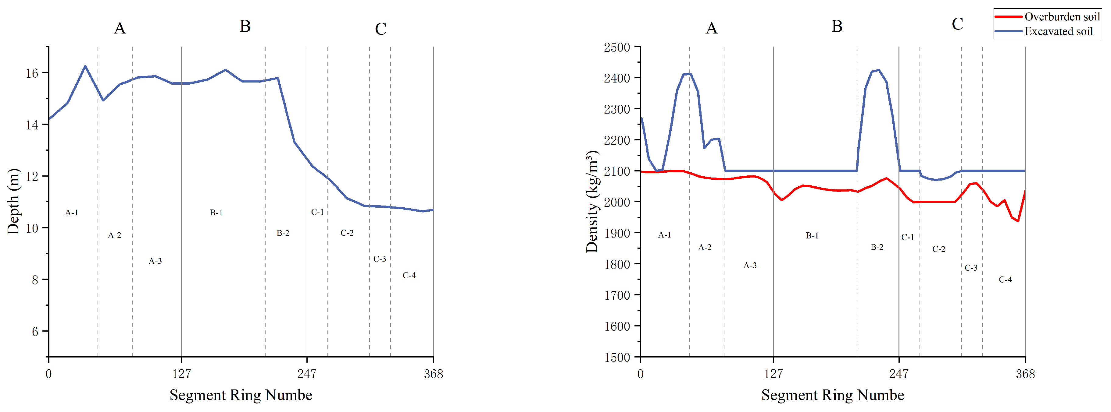
| Sections | Section Number | Ring Number Range | Overlying Soil Layer | Excavation Soil Layer |
|---|---|---|---|---|
| A | 1 | 1–47 | Completely weathered slate Highly weathered slate | Highly weathered slate Moderately weathered slate |
| 2 | 48–80 | Plain fill Completely weathered slate Highly weathered slate | Highly weathered slate Moderately weathered slate | |
| 3 | 81–127 | Plain fill Completely weathered slate Highly weathered slate | Highly weathered slate | |
| B | 1 | 128–207 | Plain fill Silty clay Completely weathered slate Highly weathered slate | Highly weathered slate |
| 2 | 208–247 | Plain fill Completely weathered slate Highly weathered slate | Highly weathered slate Moderately weathered slate | |
| C | 1 | 248–267 | Plain fill Silty clay Completely weathered slate | Highly weathered slate |
| 2 | 268–307 | Silty clay Completely weathered slate | Completely weathered slate Highly weathered slate | |
| 3 | 308–327 | Silty clay Completely weathered slate Highly weathered slate | Highly weathered slate | |
| 4 | 328–368 | Plain fill Silty clay Boulders Completely weathered slate Highly weathered slate | Highly weathered slate |
| Section | Thrust Force (kN) | Torque (kN·m) | Rotation Speed (r/min) | Thrust Speed (mm/min) |
|---|---|---|---|---|
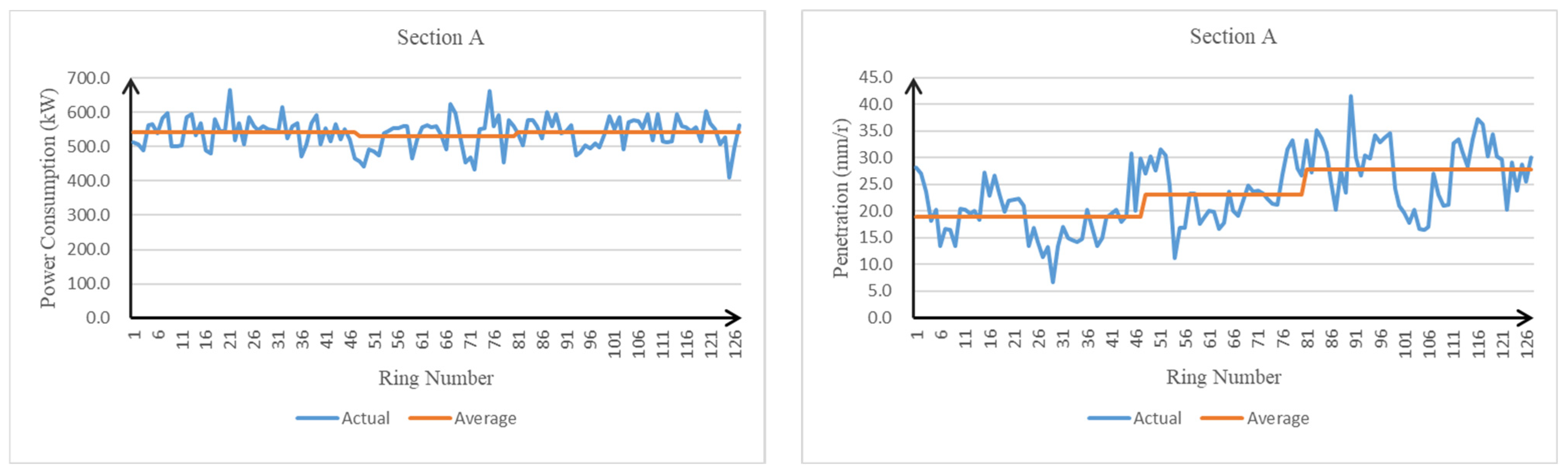
| A-1 | 14,587 | 3390 | 1.51 | 28.57 |
| A-2 | 13,710 | 3328 | 1.49 | 34.67 |
| A-3 | 15,162 | 3412 | 1.48 | 41.38 |
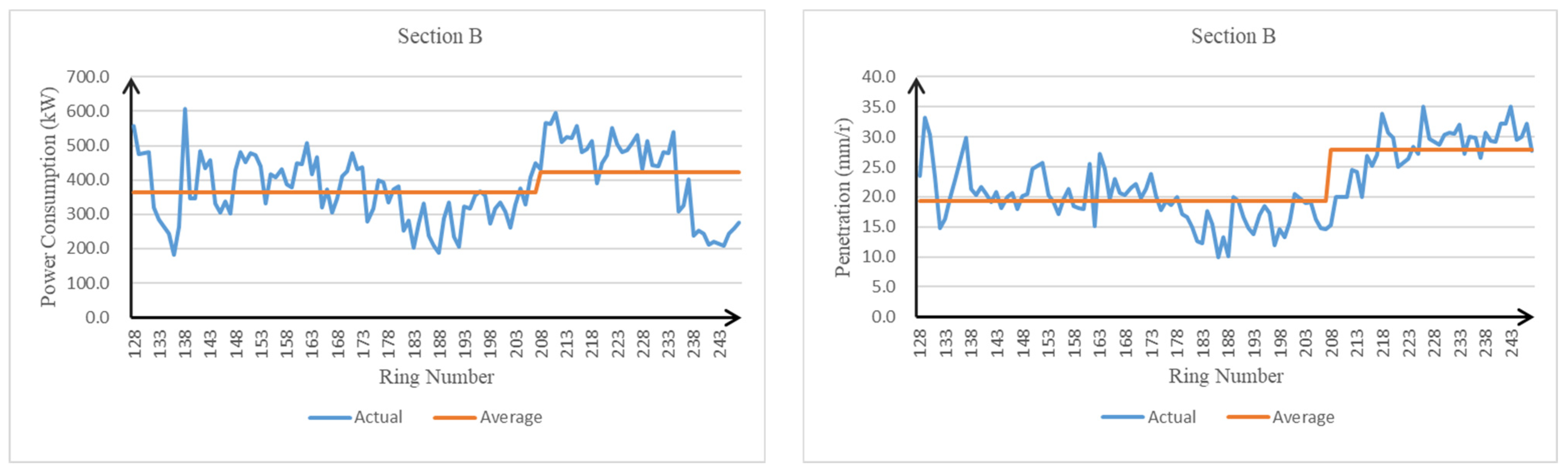
| B-1 | 12,529 | 2259 | 1.51 | 29.15 |
| B-2 | 11,535 | 2674 | 1.48 | 41.35 |
| C-1 | 11,150 | 2254 | 1.51 | 44.80 |
| C-2 | 8905 | 1470 | 1.49 | 49.10 |
| C-3 | 8475 | 1175 | 1.52 | 47.65 |
| C-4 | 10,376 | 1424 | 1.51 | 41.00 |
| Parameter Name | Parameter Value |
|---|---|
| Initial population number | 50 |
| Maximum number of iterations | 200 |
| Learning Factor c1 | 2 |
| Learning Factor c2 | 2 |
| Initial value of inertia weight | 0.9 |
| Inertial weight end value | 0.4 |
| Pareto solution set size | 50 |
| Section | Thrust Force (kN) | Torque (kN·m) | Rotation Speed (r/min) | Thrust Speed (mm/min) |
|---|---|---|---|---|
| A-1 | 13,000 | 3000 | 1.41 | 28.25 |
| A-2 | 12,000 | 2700 | 1.39 | 22.10 |
| A-3 | 11,500 | 2900 | 1.38 | 38.23 |
| Section | Thrust Force (kN) | Torque (kN·m) | Rotation Speed (r/min) | Thrust Speed (mm/min) |
|---|---|---|---|---|
| B-1 | 9000 | 1100 | 1.41 | 28.84 |
| B-2 | 11,000 | 1400 | 1.40 | 36.37 |
| C-1 | 10,000 | 1100 | 1.42 | 40.16 |
| C-2 | 9000 | 1000 | 1.43 | 42.80 |
| C-3 | 8000 | 1000 | 1.41 | 41.16 |
| C-4 | 9000 | 1200 | 1.45 | 38.56 |
| Section | Thrust Force (kN) | Torque (kN·m) | Rotation Speed (r/min) | Thrust Speed (mm/min) |
|---|---|---|---|---|
| A-1 | 13,000 | 3186 | 1.41 | 34.43 |
| A-2 | 12,000 | 3186 | 1.39 | 33.43 |
| A-3 | 11,500 | 3463 | 1.38 | 46.25 |
| B-1 | 9000 | 1250 | 1.41 | 20.00 |
| B-2 | 11,000 | 2875 | 1.40 | 40.00 |
| C-1 | 10,000 | 1729 | 1.42 | 49.00 |
| C-2 | 9000 | 1000 | 1.43 | 53.50 |
| C-3 | 8000 | 1071 | 1.41 | 48.56 |
| C-4 | 9000 | 1700 | 1.45 | 41.83 |
| Section | Total Power Consumption (kW) | Tunneling Efficiency (mm/r) | ||
|---|---|---|---|---|
| Original | Optimized | Original | Optimized | |
| A-1 | 542.8 | 477.6 | 18.9 | 24.4 |
| A-2 | 530.5 | 470.2 | 23.1 | 24.1 |
| A-3 | 542.6 | 509.1 | 27.8 | 33.5 |
| B-1 | 363.0 | 187.5 | 19.3 | 14.2 |
| B-2 | 422.2 | 428.6 | 27.9 | 28.6 |
| C-1 | 364.6 | 265.1 | 29.7 | 34.5 |
| C-2 | 236.5 | 157.7 | 33.0 | 37.4 |
| C-3 | 192.4 | 164.5 | 31.6 | 34.4 |
| C-4 | 232.2 | 264.3 | 27.2 | 28.8 |
Disclaimer/Publisher’s Note: The statements, opinions and data contained in all publications are solely those of the individual author(s) and contributor(s) and not of MDPI and/or the editor(s). MDPI and/or the editor(s) disclaim responsibility for any injury to people or property resulting from any ideas, methods, instructions or products referred to in the content. |
© 2024 by the authors. Licensee MDPI, Basel, Switzerland. This article is an open access article distributed under the terms and conditions of the Creative Commons Attribution (CC BY) license (https://creativecommons.org/licenses/by/4.0/).
Share and Cite
Wang, W.; Feng, H.; Li, Y.; Zheng, X.; Qi, J.; Sun, H. Research on Multi-Objective Optimization of Shield Tunneling Parameters Based on Power Consumption and Efficiency. Sustainability 2024, 16, 6152. https://doi.org/10.3390/su16146152
Wang W, Feng H, Li Y, Zheng X, Qi J, Sun H. Research on Multi-Objective Optimization of Shield Tunneling Parameters Based on Power Consumption and Efficiency. Sustainability. 2024; 16(14):6152. https://doi.org/10.3390/su16146152
Chicago/Turabian StyleWang, Wei, Huanhuan Feng, Yanzong Li, Xudong Zheng, Jinhui Qi, and Huaize Sun. 2024. "Research on Multi-Objective Optimization of Shield Tunneling Parameters Based on Power Consumption and Efficiency" Sustainability 16, no. 14: 6152. https://doi.org/10.3390/su16146152