Article

Regional Truck Travel Characteristics Analysis and Freight Volume Estimation: Support for the Sustainable Development of Freight

1
Planning and Research Institute, Ministry of Transport, Beijing 100028, China
2
Key Laboratory of Intelligent Police of Sichuan Province, Sichuan Police College, Luzhou 646000, China
3
College of Metropolitan Transportation, Beijing University of Technology, Beijing 100124, China
*
Author to whom correspondence should be addressed.
Sustainability 2024, 16(15), 6317; https://doi.org/10.3390/su16156317
Submission received: 2 July 2024 / Revised: 18 July 2024 / Accepted: 22 July 2024 / Published: 24 July 2024

Abstract

:
In the field of freight transport, the goal of sustainable development requires us to improve the efficiency of freight transport while reducing its negative impact on the environment, such as reducing carbon emissions and noise pollution. There is no doubt that changes in freight characteristics and volumes are compatible with the objectives of sustainable development. Thus, mining the travel distribution and freight volume of trucks has an important supporting role in the freight transport industry. In terms of truck travel, most of the traditional approaches are based on the subjective definition of parameters from the trajectory data to obtain trips for certain vehicle types. As for freight volume, it is mostly estimated through manual surveys, which are heavy and inaccurate. In this study, a data-driven approach is adopted to obtain trips from the trajectory data of heavy trucks. Combined with the traffic percentage of different vehicle types collected by highway traffic survey stations, the trips of heavy trucks are extended to all trucks. The inter-city and intra-city freight volumes are estimated based on the average truck loads collected at the motorway entrance. The results show a higher proportion of intra-city trips by trucks in port cities and a higher proportion of inter-city trips by trucks in inland cities. Truck loading and unloading times are focused in the early morning or at night, and freight demand in Shandong Province is more concentrated in the south. These results would provide strong support for optimizing freight structures, improving transportation efficiency, and reducing transportation costs.

1. Introduction

Freight transport is a significant contributor to air pollutants and greenhouse gas emissions. Under the concept of sustainable development, the Chinese government has introduced a series of policies in recent years and is formulating plans for environmental protection, carbon reduction, and transportation development for the next five years. Freight restructuring forms an important part of these policies and plans. In order to ensure the rationality of freight structure adjustment, we first need to comprehensively and accurately grasp the freight distribution and freight volume demand [1].
In recent years, inter-city freight capacity has been increasing due to the promotion of supply-side structural reforms and various emergencies [2,3]. The structure of freight transport has changed from a decentralized layout to a centralized logistics hub [4]. With the increasing demand for logistics transportation as the main means of transport between industrial production enterprises and warehouses, trucks will play an increasingly important role in inter-city freight [5]. In turn, the travel characteristics of trucks will have an impact on road network planning, logistics hub design, road maintenance, and road safety [6]. Therefore, it is important to understand the distribution of trucking trips and freight volumes.
The first challenge is to obtain reliable and accurate data on truck trips with a wide coverage. Traditionally, truck trips are collected manually through questionnaires or stop-and-asks [7]. However, there are shortcomings, such as the under-representation of samples, long time periods, and poor accuracy [8,9]. In addition, license plate recognition technology can also be used to infer the macro chain of vehicle travel [10], but it is difficult to obtain a fine-grained driving trajectory from it. With the widespread use of the Global Positioning System (GPS), the transportation industry has generated a large amount of truck trajectory data with temporal, spatial, and other properties. In order to mine valuable information, it is necessary to extract trips from the trajectory data.
Currently, the mainstream method for extracting trip trajectory data is to identify the stopping points of trucks by setting the appropriate thresholds [11]. And then, the filtering conditions are set to identify the trip end points from the numerous stopping points. Identifying the stopping points means finding the point at which the truck is stationary. When the truck is stationary, its speed should be 0. However, considering the drift of the signal collected by the device, the speed may be very low when the truck is stationary [12]. Therefore, it is necessary to define a threshold value. If the speed is lower than the threshold value, the truck is considered to be stationary. Most previous studies have defined speed thresholds based on personal experience [13]. End-of-trip identification, on the other hand, is about recognizing the end of the trip from the stopping points. Previous research has mostly relied on the empirical definition of dwell time thresholds [14]. The dwell time for each stop is counted. If the threshold is exceeded, the truck is considered to have completed the trip; otherwise, it is a temporary stop of the trip. However, the subjective setting of the threshold value would lead to bias in the identification results. At the same time, the analysis results are under-representative as it is difficult to obtain the trajectory data of all the trucks.
The second challenge is the statistics of inter-city road freight volumes. As an important component of transport statistics, road freight volume is an important metric that reflects the present and future development trends in the regional economy [15,16]. The traditional way of measuring freight volume statistics is that the key freight enterprises report monthly and the statistical department combines fixed coefficients to expand the sample of the results [17]. While the key freight transport enterprises only account for a part of the transport market share, the market share of these enterprises is constantly changing due to economic fluctuations; therefore, this statistical method has certain defects. To improve statistical accuracy, some studies have supplemented the use of multiple sources of data, such as postal information, on-board OBD equipment, and freight yards [18,19]. However, these studies have focused on characteristics analysis or demand forecasting, not addressing the issue of freight volume statistics. The results of inter-city road freight volumes are difficult to calculate accurately due to the lack of access to truth values.
In this study, a data-driven approach is adopted to obtain trips based on heavy truck trajectory data. By combining the proportions of different truck types in the road traffic survey collection data, the trips are expanded to all truck types, thus obtaining the Origin–Destination (OD) matrix for inter-city and intra-city truck trips. Based on the weighing data of trucks collected at motorway entrances, average truck loads are calculated. Finally, the inter-city road freight volumes are obtained by combining the inter-city truck OD matrices and the average loads. The research results reveal the spatial and temporal distribution of freight travel between cities and show the difference in freight demand, which provides strong support for the optimization of freight structures.
The rest of this paper is structured as follows. Section 2 provides the characteristics of the studied data, followed by the data processing in Section 3. Section 4 introduces the computational frameworks, including travel chain identification, trip chain expansion, and freight volume estimation. Section 5 presents the analysis results and discussions. Section 6 summarizes the conclusions.

2. Data Characteristics

The heavy truck trajectory data used in this study were obtained from local transport authorities. The Ministry of Transport requires the installation of satellite positioning devices with the function of tachographs on trucks operating over 12 tons. The collected truck location information is continuously transmitted to the unified management platform to ensure road safety. The data range used in the study was one week of heavy truck trajectory data from 1 August to 7 August 2021 in Shandong Province, with a collection interval of 30 s. Statistically, a total of 470,000 heavy trucks traveled in Shandong Province during this period, generating 2.5 billion pieces of trajectory data. The trajectory sample data are shown in Table 1.
The traffic percentages of the different vehicle types were obtained from the National Highway Network Traffic Survey Data Collection and Services System. To obtain real-time road traffic data, each local transport authority installs automated roadside survey stations and collects the number of vehicles passing the stations by vehicle type. Data collected by the survey stations are transmitted to the unified management system at five-minute intervals.
Meanwhile, the weighing data of trucks passing through motorway entrances were used in this study. To strengthen the control of illegal overloading on highways, weighing equipment has been installed at the entrances of motorways nationwide. When the truck passes through the entrance, information such as the truck ID, number of axles, weight of the load, and traveling time is collected.

3. Data Processing

Raw GPS trajectory data are unusable due to the presence of errors. The pre-processing of the data is, therefore, required. Typical erroneous data include data duplication, abnormal data drift, and data loss.
For data duplication, if a vehicle collects two consecutive trajectory data, but at the same time and location, only the first duplicate is kept, and subsequent duplicates are deleted. For abnormal drift data, we first calculate the interval speed v ¯ between successive trajectories. Given two continuous trajectory points of vehicle u , P u ( l o n i , l a t i , t i ) and P u ( l o n i + 1 , l a t i + 1 , t i + 1 ) , the interval speed of the i + 1 th point is calculated as follows:
v ¯ u , i + 1 = D u , i + 1 / ( t i + 1 t i )
where D u , i + 1 is the geospatial distance calculated based on the latitude and longitude of the two successive points.
When the interval speed between two points far exceeds the maximum speed allowed for trucks on the road, e.g., 180 km/h, then at least one of the points is abnormally drifting. If the speed exceeds 180 km/h in two consecutive intervals, the GPS record is rejected in the middle of the interval. If only one interval speed exceeds this limit, it is temporarily ignored and handled by setting a threshold for the number of track points during the trip screening.
For data loss, there are two scenarios. In the first case, the device runs abnormally and the spatial information is empty; then, the record is deleted directly [20]. In the second case, where the device has no signal for more than 1 h, the anomaly is likewise temporarily ignored and dealt with during trip screening. After data processing, the heat distribution of GPS track driving in Shandong Province is shown in the figure. After data processing and data normalization, the trajectory heat distribution of heavy trucks running in Shandong Province is shown in Figure 1.

4. Methodology

4.1. Travel Chain Identification

We identify the travel chain of each truck in two steps. Firstly, rules are established to determine the stopping points of the truck from the trajectory data. The second step is to identify the start and end points of the trip from the stopping points and eventually obtain the OD matrix for inter-city trips.

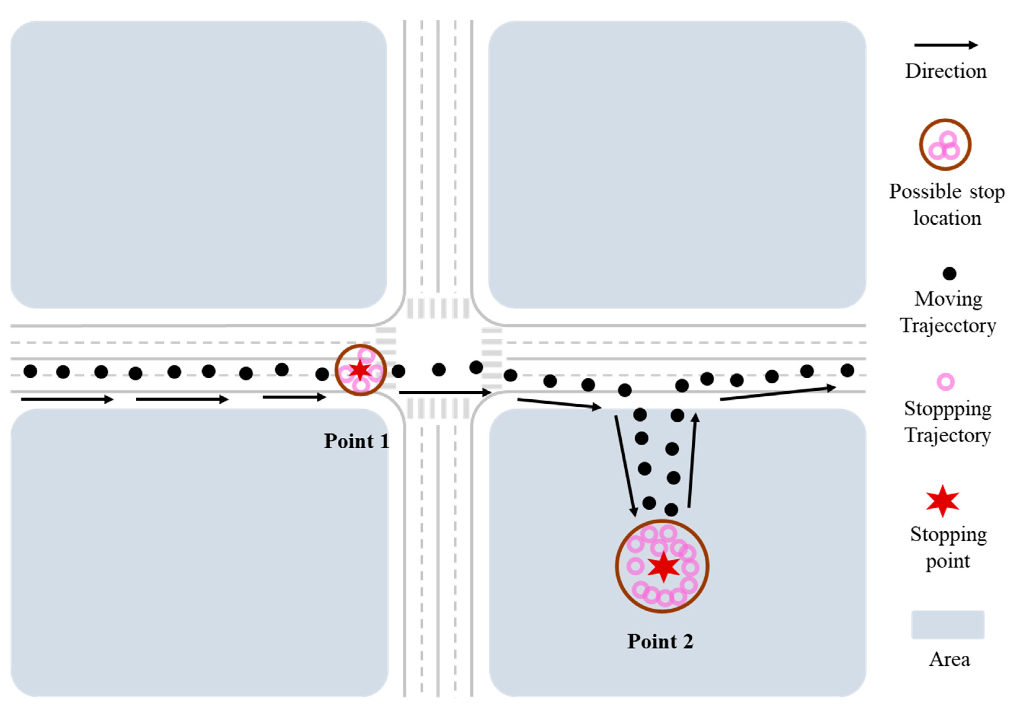
4.1.1. Stopping Point Identification

The truck stopping point means that the truck has stopped at a certain location for a period of time. Normally, the interval speed should be 0 when the truck stops. However, the accuracy of civilian positioning devices is generally below 10 m [21]. Therefore, even if a vehicle is stationary for a period of time, the latitude and longitude information collected during that period will be slightly different, as shown in Figure 2. In order to reduce the error caused by trajectory drift, it is necessary to define a speed threshold to determine the vehicle’s traveling state.
As we know, the stopping point is not only a stationary point but also a moving point at a low speed in a certain area (such as a freight transit station). Therefore, all the track data include different travel characteristics or modes, so the distribution of travel speed is most suitable for a Gaussian mixture distribution. In this study, truck stopping points are identified by constructing a Gaussian Mixture Model (GMM). By randomly selecting the interval speed of 10,000 heavy trucks, we obtained the interval speed distribution and displayed it on a double-logarithmic axis. As shown by the pink circle in Figure 3, there are two peaks in the speed distribution. According to previous studies, the right peak distribution can be assumed to represent the speed characteristics of the vehicle during normal traveling, while the left peak distribution is mainly caused by trajectory drift [22]. As shown in Equation (2), a GMM is constructed by taking the speeds of the two states, drift and normal traveling, as the distribution base.
f x = λ 1 1 x σ 1 2 π exp ln x μ 1 2 2 σ 1 2 + λ 2 1 σ 2 2 π exp ( x μ 2 ) 2 2 σ 2 2
where f x denotes the probability density function of the GMM; λ 1 and λ 2 are the weights of the GMM. μ 1 , μ 2 , σ 1 , and σ 2 are the parameters of the two probability distributions and can be estimated by maximizing the likelihood [23]. The results of the parameter estimation and the fitted Gaussian mixture distribution (the solid line) are presented in Figure 3. The lowest point in the middle of the bimodal curve is known as the saddle point, where the entire distribution is divided into two parts. The value of the saddle point is the threshold for determining the driving state of the vehicle. When the speed exceeds the threshold, it indicates that the truck is traveling, and when it is less than the threshold, it indicates that the truck is stopped. Based on the constructed GMM, the speed threshold for heavy trucks in Shandong Province is 0.973 km/h.
A heavy truck will produce a significant number of trajectories in close proximity to the stopping point due to signal drift. By calculating the average value of the longitude and latitude of all trajectories within the stopping point, the specific location of the stopping point can be obtained, as shown by the pentagram in Figure 2.

4.1.2. Trip Identification

Based on the dwell time of the trucks at the stopping points calculated in the previous step, we obtained the average dwell time distribution of heavy trucks. It is displayed in double logarithmic axes, as shown by the circles in Figure 4. It can be clearly found that the dwell time distribution is trinomial. By great likelihood fitting, a three-segmented power law function (the solid line) can be obtained with 148 min and 462 min as the broken points [24]. Broken power law functions are concepts from statistical physics that are now being increasingly used in the natural sciences, biology, and economics in an attempt to understand and model the large variability and risk in phenomena [25,26,27].
For heavy trucks, there are three main stopping states: temporary parking, the loading and unloading of goods, and the end of the trip. There are many reasons for temporary parking, such as road congestion, refueling, drivers eating, etc. [28]. As shown by point 1 in Figure 5, temporary parking stops are generally short and are not the end of the trip. Heavy trucks generally stay longer when loading and unloading goods, as shown by point 2 in Figure 5. Because of the large amount of goods loaded and unloaded in heavy trucks, equipment is usually required to assist in the operation. The dwell time would, therefore, be significantly longer than that of temporary parking. Finally, heavy trucks would stay for a very long time at the end of their trip. The three stopping states correspond to the three segments of the power law function shown in Figure 4. Therefore, when the dwell time of a heavy truck is less than 148 min, it is judged to be temporary parking. When the dwell time is between 148 min and 462 min, it is judged to be loading or unloading goods. If the dwell time exceeds 462 min, it is judged to be an end-of-trip. In this study, we chose to ignore all stopping points with temporary parking and extracted stopping points with a dwell time of more than 148 min as the end of the trip.
Based on the above principles, we extract the start and end points of each trip from the trajectory data of the heavy truck. Through map matching, the inter-city travel chain of each truck can then be obtained. Figure 6 shows an example of a travel chain result in which we use a green dot for the starting point, black dots for important points, red dots for moving points, and a star sign for the stopping point. Specifically, the selected truck made a stop at a gas station.
We define the travel chain of truck u as t r i p u o i , d j , t , u = 1 , 2 , , n , where o i , i = 1 , 2 , , k and d j , j = 1 , 2 , , k represent the starting and ending cities of the trip, respectively; t represents the departure time of the trip. In order to delete trips generated by the signal drift and temporary movement of heavy trucks, only trips with more than 10 trajectory points are retained [29]. With the departure city, arrival city, and departure time as three characteristics, the trajectory data of heavy trucks are aggregated into a three-dimensional matrix M T R 3 , in which each element m T o i , d j , h denotes the number of trips made by the heavy trucks from the city o i to city d j in h hours of the day.

4.2. Trip Chain Expansion

Using the travel chain of heavy-duty trucks to infer the global truck travel chain is the key to a comprehensive understanding of freight distribution. The vehicle detection data from the National Highway Network Traffic Survey Data Collection and Services System provide a solution to this problem. The detection data recorded the type of each passing vehicle; thereby, the percentage of different vehicle types can be obtained. The collected truck types included small trucks, medium trucks, large trucks, extra-large trucks, and containers. Table 2 shows the percentage of different types of trucks from 1–7 August 2021. According to the standard specification of the traffic survey collection model, large trucks, extra-large trucks, and containers are classified as heavy trucks with a percentage ρ = 61.6 % of the total number of trucks. Thus, the OD matrix M = M T / ρ is obtained for the entire truck trip in Shandong Province.

4.3. Freight Volume Estimation

In order to estimate inter-city road freight volumes, it is first necessary to obtain the average load capacity of each truck. In this study, the average load capacity of trucks is estimated based on the weighing data of trucks at motorway entrances. The weighing equipment classifies trucks according to the number of axles, which is inconsistent with the criteria used in the highway traffic survey. We, therefore, take the traffic percentage of different truck types with each axle number as a weight, combine it with the average load capacity of trucks with each axle number, and then estimate the average load capacity of trucks. Based on the weight distribution of trucks for each axle number, the average load capacity α i , x and traffic percentage δ i , x for each number of axles x , x = 1 , 2 , , n in each city i are calculated. Finally, we obtain the average load capacity of trucks in each city α i = x = 1 n α i , x · δ i , x . Combined with the OD matrix of truck trips, the inter-city average daily freight volume matrix W i , j = α i · h = 1 24 M i , j can be obtained. The element w o i , d j denotes the average daily freight volume from city o i to city d j .

5. Results and Discussion

5.1. Truck Travel Characteristics

This study uses trajectory data of 471,000 heavy trucks traveling in Shandong Province to obtain inter-city OD matrices. Together with the traffic percentage of different vehicle types collected from about 1000 highway traffic survey stations, we finally obtain the inter-city OD matrix of trucks traveling in Shandong Province.
For cities, we classify truck trips into three modes: trips inside the city, trips to other cities, and trips from other cities. The volume of truck trips and the percentage of truck trips by mode in each city are shown in Figure 7. A larger pie chart radius indicates more truck trips. The results show that trucks are mainly active in the cities of Linyi, Weifang, and Qingdao. Among them, Linyi, as the logistics capital of China, is the largest distribution center for commodities in northern China and has the highest number of truck trips [30]. Due to the large number and dispersed distribution nodes of freight transport in Linyi, there is a high demand for transport between the nodes, resulting in a large proportion of intra-city trips.
On the other hand, there are major differences in the characteristics of truck trips between coastal and inland cities. For Qingdao, Yantai, and Weihai, as they are port cities, many containers, iron ore, and other goods are transported to the freight yards by rail [31]. This results in a smaller proportion of road truck trips to other cities and more intra-city road trips between ports and freight yards. For inland cities, such as Jinan, Zibo, Tai’an, etc., trucks are engaged in more inter-city traveling, and the proportion of intra-city travel is only about one-third. These results show that freight traffic is closely related to local economic development and that freight traffic between cities is becoming more and more intense.
The distribution of departure and arrival times of trucks throughout the day is shown in Figure 8. It can be found that trucks start preparing for transport as early as 3 a.m., with departure times concentrated between 5 a.m. and 9 a.m., while fewer departures take place in the afternoon. In terms of arrival times, there are two peaks at 12:00 and 19:00, and they are relatively concentrated in the first half of the night and taper off after 23:00. There is only one significant peak in departure times, reflecting the fact that most trucks will only make a single trip per day. And, in order to improve the efficiency of transport, trucks are mostly loaded and unloaded in the early morning or at night so as to reduce the impact of social activities on transport.

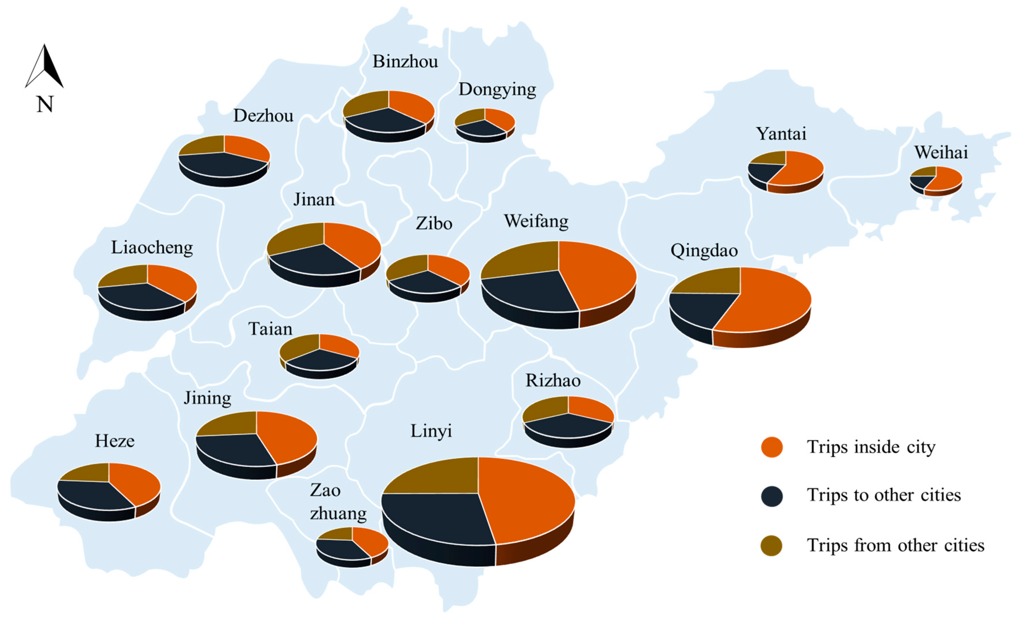
5.2. Analysis of Inter-City Freight Volumes

Knowledge of inter-city freight volumes can help better analyze truck travel behavior [32]. Combined with the weighing data of trucks at motorway entrances, the magnitude of inter-city loads is inferred and normalized, as shown in Figure 9. Obviously, Heze–Jining, Linyi–Rizhao, and Qingdao–Weifang are the three sets of city pairs with the largest inter-city freight traffic. Due to the developed water system in Jining City, with the help of the Beijing–Hangzhou Canal, a large amount of coal and a large number of containers are transported to Jining through Heze, ultimately serving the development of the Yangtze River Delta region, resulting in a very large freight volume between Heze and Jining. Linyi–Rizhao and Qingdao–Weifang have large freight volumes because all four cities are nationally important logistics hubs. In addition, from the perspective of spatial distribution, the freight volume of southern cities in Shandong Province is significantly higher than that of northern cities.

6. Conclusions

Understanding the proportion of different freight volumes and changing trends will help optimize the transportation structure, improve transportation efficiency, reduce transportation costs, and reduce the impact on the environment. This study calculates the intra-city and inter-city OD travel matrix of heavy trucks in Shandong Province based on trajectory data using a data-driven approach. Combined with the traffic percentage of different vehicle types collected by highway traffic survey stations, the trips of heavy trucks were extended to all trucks. Finally, the average truck loads in each municipality were extracted based on the motorway entrance weighing data.
The results of the study show that (1) as a result of the structural reform of the transport supply side, port cities have a higher proportion of intra-city trips by trucks; (2) trucks in port cities are more likely to serve between freight yards and ports; (3) inland cities have a higher proportion of inter-city trips by trucks; (4) in order to improve transport efficiency, the loading and unloading of goods by trucks is staggered to coincide with the main activities of the community; and (5) related to the level of economic development, freight demand in Shandong Province is more concentrated in the southern region. Among them, Linyi, as the logistics capital of China, has a strong demand for freight transport with its neighboring cities.
The inter-city freight distribution and freight volumes obtained from this study can help visually analyze local freight characteristics. For example, it can provide basic data support for regional integrated transport planning. The planning and deployment of logistics distribution nodes also need to refer to the distribution of freight. At the same time, road infrastructure, road maintenance and safety, and emergency response can be targeted to develop preventive measures based on freight distribution characteristics.
There are also some areas for improvement in this study. For instance, when expending a sample of a truck’s trip, there may be some differences in the driving characteristics of heavy trucks and small trucks in different seasons. Also, when calculating the average load capacity of trucks, there may also be differences between trucks on motorways and ordinary roads. However, at this stage, there is no way of obtaining the travel path and load capacity of the full volume of trucks, so this part of the effect is ignored in this study.

Author Contributions

Conceptualization, S.L.; Software, J.O.; Validation, M.G. and S.L.; Formal analysis, S.S.; Investigation, S.S.; Resources, M.G.; Data curation, J.O. and Z.L.; Writing—original draft, S.S.; Writing—review & editing, S.L.; Funding acquisition, Z.L. and S.L. All authors have read and agreed to the published version of the manuscript.

Funding

This study is supported by the Technology Development Project of Transport Planning and Research Institute (Grant no. 092223-322) and the Beijing Postdoctoral Foundation (Grant no. 2023-zz-134).

Institutional Review Board Statement

Not applicable.

Informed Consent Statement

Not applicable.

Data Availability Statement

The data used to support the findings of this study are available from the corresponding author upon reasonable request.

Conflicts of Interest

The authors declare that they have no conflicts of interest regarding the publication of this article.

References

  1. Flamini, M.; Nigro, M.; Pacciarelli, D. The value of real-time traffic information in urban freight distribution. J. Intell. Transp. Syst. 2018, 22, 26–39. [Google Scholar] [CrossRef]
  2. Balla, B.S.; Sahu, P.K. Assessing regional transferability and updating of freight generation models to reduce sample size requirements in national freight data collection program. Transp. Res. Part APolicy Pract. 2023, 175, 103780. [Google Scholar] [CrossRef]
  3. Yin, C.; Zhang, Z.; Zhang, X.; Chen, J.; Tao, X.; Yang, L. Hub seaport multimodal freight transport network design: Perspective of regional integration development. Ocean Coast. Manag. 2023, 242, 106675. [Google Scholar] [CrossRef]
  4. Akhavan, M.; Ghiara, H.; Mariotti, I.; Sillig, C. Logistics global network connectivity and its determinants. A European City network analysis. J. Transp. Geogr. 2020, 82, 102624. [Google Scholar] [CrossRef]
  5. Yang, Y.; Jia, B.; Yan, X.Y.; Li, J.; Yang, Z.; Gao, Z. Identifying intercity freight trip ends of heavy trucks from GPS data. Transp. Res. Part E Logist. Transp. Rev. 2022, 157, 102590. [Google Scholar] [CrossRef]
  6. Cassiano, D.R.; Bertoncini, B.V.; de Oliveira, L.K. A conceptual model based on the activity system and transportation system for sustainability urban freight transport. Sustainability 2021, 13, 5642. [Google Scholar] [CrossRef]
  7. Nuzzolo, A.; Crisalli, U.; Comi, A. A restocking tour model for the estimation of OD freight vehicle in urban areas. Procedia-Soc. Behav. Sci. 2011, 20, 140–149. [Google Scholar] [CrossRef]
  8. Toilier, F.; Gardrat, M. Driver survey vs GPS Tour data: Strength and weaknesses of the two sources in order to model the drivers’ journeys. Transp. Res. Procedia 2024, 76, 169–182. [Google Scholar] [CrossRef]
  9. Demissie, M.G.; Kattan, L. Estimation of truck origin-destination flows using GPS data. Transp. Res. Part E Logist. Transp. Rev. 2022, 159, 102621. [Google Scholar] [CrossRef]
  10. Siripirote, T.; Sumalee, A.; Watling, D.P.; Shao, H. Updating of travel behavior model parameters and estimation of vehicle trip chain based on plate scanning. J. Intell. Transp. Syst. 2014, 18, 393–409. [Google Scholar] [CrossRef]
  11. Adam, A.; Finance, O.; Thomas, I. Monitoring trucks to reveal Belgian geographical structures and dynamics: From GPS traces to spatial interactions. J. Transp. Geogr. 2021, 91, 102977. [Google Scholar] [CrossRef]
  12. Van Dijk, J. Identifying activity-travel points from GPS-data with multiple moving windows. Comput. Environ. Urban Syst. 2018, 70, 84–101. [Google Scholar] [CrossRef]
  13. Laranjeiro, P.F.; Merchán, D.; Godoy, L.A.; Giannotti, M.; Yoshizaki, H.T.; Winkenbach, M.; Cunha, C.B. Using GPS data to explore speed patterns and temporal fluctuations in urban logistics: The case of São Paulo, Brazil. J. Transp. Geogr. 2019, 76, 114–129. [Google Scholar] [CrossRef]
  14. He, Z.; Zhao, P.; Xiao, Z.; Huang, X.; Li, Z.; Kang, T. Exploring the distance decay in port hinterlands under port regionalization using truck GPS data. Transp. Res. Part E Logist. Transp. Rev. 2024, 181, 103390. [Google Scholar] [CrossRef]
  15. Darayi, M.; Barker, K.; Nicholson, C.D. A multi-industry economic impact perspective on adaptive capacity planning in a freight transportation network. Int. J. Prod. Econ. 2019, 208, 356–368. [Google Scholar] [CrossRef]
  16. Chupin, A.; Morkovkin, D.; Bolsunovskaya, M.; Boyko, A.; Leksashov, A. Techno-Economic Sustainability Potential of Large-Scale Systems: Forecasting Intermodal Freight Transportation Volumes. Sustainability 2024, 16, 1265. [Google Scholar] [CrossRef]
  17. Jin, W.Z.; Zhang, Q. Study on Regional Freight Transportation Investigation and Statistics. J. Highw. Transp. Res. Dev. 2005, 04, 139–143. [Google Scholar]
  18. Müller, S.; Wolfermann, A.; Huber, S. A nation-wide macroscopic freight traffic model. Procedia-Soc. Behav. Sci. 2012, 54, 221–230. [Google Scholar] [CrossRef]
  19. Hassan, L.A.H.; Mahmassani, H.S.; Chen, Y. Reinforcement learning framework for freight demand forecasting to support operational planning decisions. Transp. Res. Part E Logist. Transp. Rev. 2020, 137, 101926. [Google Scholar] [CrossRef]
  20. Miller, S.; Vander Laan, Z.; Marković, N. Scaling GPS trajectories to match point traffic counts: A convex programming approach and Utah case study. Transp. Res. Part E Logist. Transp. Rev. 2020, 143, 102105. [Google Scholar] [CrossRef]
  21. Li, F.; Tu, R.; Zeng, L.; Zhang, S.; Liu, M.; Lu, X. Integrated positioning with double-differenced 5G and undifferenced/double-differenced GPS. Measurement 2023, 218, 113114. [Google Scholar] [CrossRef]
  22. Lyu, Z.; Pons, D.; Zhang, Y.; Ji, Z. Freight Operations Modelling for Urban Delivery and Pickup with Flexible Routing: Cluster Transport Modelling Incorporating Discrete-Event Simulation and GIS. Infrastructures. 2021, 6, 180. [Google Scholar] [CrossRef]
  23. Orellana, R.; Carvajal, R.; Juan, C.A. Maximum Likelihood Infinite Mixture Distribution Estimation Utilizing Finite Gaussian Mixtures—ScienceDirect. IFAC-PapersOnLine 2018, 51, 706–711. [Google Scholar] [CrossRef]
  24. Manole, T.; Khalili, A. Estimating the number of components in finite mixture models via the group-sort-fuse procedure. Ann. Stat. 2021, 49, 3043–3069. [Google Scholar] [CrossRef]
  25. Sornette, D. Critical Phenomena in Natural Sciences: Chaos, Fractals, Selforganization and Disorder: Concepts and Tools; Springer Science & Business Media: Berlin/Heidelberg, Germany, 2006. [Google Scholar]
  26. Marković, D.; Gros, C. Power laws and self-organized criticality in theory and nature. Phys. Rep. 2014, 536, 41–74. [Google Scholar] [CrossRef]
  27. Chehade, A.; Shi, Z.; Krivtsov, V. Power–law nonhomogeneous Poisson process with a mixture of latent common shape parameters. Reliab. Eng. Syst. Saf. 2020, 203, 107097. [Google Scholar] [CrossRef]
  28. Gingerich, K.; Maoh, H.; Anderson, W. Classifying the purpose of stopped truck events: An application of entropy to GPS data. Transp. Res. Part C: Emerg. Technol. 2016, 64, 17–27. [Google Scholar] [CrossRef]
  29. Łukawska, M.; Paulsen, M.; Rasmussen, T.K.; Jensen, A.F.; Nielsen, O.A. A joint bicycle route choice model for various cycling frequencies and trip distances based on a large crowdsourced GPS dataset. Transp. Res. Part A Policy Pract. 2023, 176, 103834. [Google Scholar] [CrossRef]
  30. Wang, G.; Qian, Y.; Kong, F.; Liu, X.; Liu, Y.; Zhu, Z.; Gao, W.; Zhang, H.; Wang, Y. Non-methane hydrocarbon characteristics and their ozone and secondary organic aerosol formation potentials and sources in the plate and logistics capital of China. Atmos. Pollut. Res. 2023, 14, 101873. [Google Scholar] [CrossRef]
  31. Cong, L.Z.; Zhang, D.; Wang, M.L.; Xu, H.F.; Li, L. The role of ports in the economic development of port cities: Panel evidence from China. Transp. Policy 2020, 90, 13–21. [Google Scholar] [CrossRef]
  32. He, Z.; Liu, Q.; Zhao, P. Challenges of passenger and freight transportation in mega-city regions: A systematic literature review. Transp. Res. Interdiscip. Perspect. 2022, 16, 100730. [Google Scholar] [CrossRef]
Figure 1. Trajectory heat distribution of heavy trucks after data normalization.
Sustainability 16 06317 g001
Figure 2. Schematic diagram of vehicle trajectory with stopping points.
Sustainability 16 06317 g002
Figure 3. Interval speed distribution of heavy trucks.
Sustainability 16 06317 g003
Figure 4. Dwell time distribution of heavy trucks.
Sustainability 16 06317 g004
Figure 5. Distribution of trajectories under different parking types for truck trips.
Sustainability 16 06317 g005
Figure 6. The sample results of a travel chain from a truck.
Sustainability 16 06317 g006
Figure 7. The volume of truck trips and the percentage of truck trip mode.
Sustainability 16 06317 g007
Figure 8. The distribution of the departure and arrival times of trucks throughout the day.
Sustainability 16 06317 g008
Figure 9. Expectation line graph of normalized inter-city freight volume in Shandong.
Sustainability 16 06317 g009
Table 1. Heavy truck trajectory sample data.
Heavy Truck IDTimestampLongitudeLatitude
***** 4E2021-08-01 00:08:47117.82033536.07616
***** 4E2021-08-01 00:09:17117.82033536.07617
***** 4E2021-08-01 00:09:47117.8203336.076176
***** 4E2021-08-01 00:10:17117.8203236.076157
***** 4E2021-08-01 00:10:47117.8203336.076202
Note: the heavy truck ID is encrypted with “*****”.
Table 2. The traffic percentage of various truck types.
Truck TypeSmall TruckMedium TruckLarge TruckExtra-Large TruckContainer
Vehicle attributes2 axels
maximum
18 tons
3 axels
maximum
27 tons
4 axels
maximum
36 tons
5 axels
maximum
43 tons
6 axels
maximum
49 tons
Percentage of truck types (%)25.213.214.143.44.1
Disclaimer/Publisher’s Note: The statements, opinions and data contained in all publications are solely those of the individual author(s) and contributor(s) and not of MDPI and/or the editor(s). MDPI and/or the editor(s) disclaim responsibility for any injury to people or property resulting from any ideas, methods, instructions or products referred to in the content.

