Abstract
The digitalization of the global landscape of electricity consumption, combined with the impact of the pandemic and the implementation of lockdown measures, has required the development of a precise forecast of energy consumption to optimize the management of energy resources, particularly in pandemic contexts. To address this, this research introduces a novel forecasting model, the robust multivariate multilayered long- and short-term memory model with knowledge injection (), to improve the accuracy of forecasting models under uncertain conditions. This innovative model extends the capabilities of by incorporating an additional branch to extract energy consumption from adversarial noise. The experiment results show that demonstrates substantial improvements over and other models with adversarial training: multivariate multilayered long short-term memory (adv-M-LSTM), long short-term memory (adv-LSTM), bidirectional long short-term memory (adv-Bi-LSTM), and linear regression (adv-LR). The maximum noise level from the adversarial examples is 0.005. On average, across three datasets, the proposed model improves about 24.01% in mean percentage absolute error (MPAE), 18.43% in normalized root mean square error (NRMSE), and 8.53% in over . In addition, the proposed model outperforms “adv-” models with MPAE improvements ranging from 35.74% to 89.80% across the datasets. In terms of NRMSE, improvements range from 36.76% to 80.00%. Furthermore, achieves remarkable improvements in the score, ranging from 17.35% to 119.63%. The results indicate that the proposed model enhances overall accuracy while effectively mitigating the potential reduction in accuracy often associated with adversarial training models. By incorporating adversarial noise and COVID-19 case data, the proposed model demonstrates improved accuracy and robustness in forecasting energy consumption under uncertain conditions. This enhanced predictive capability will enable energy managers and policymakers to better anticipate and respond to fluctuations in energy demand during pandemics, ensuring more resilient and efficient energy systems.
1. Introduction
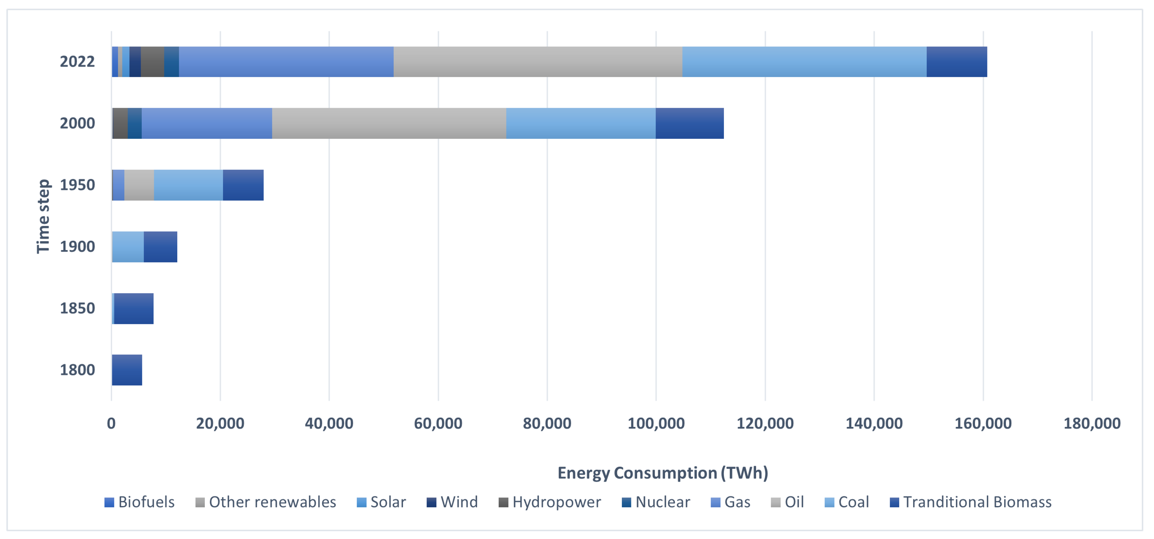
In the past century, the world’s population has experienced unprecedented growth. According to the predictions of Sadigov et al. in 2022 [1], the global population is projected to rise to an estimated 14.7 billion in the upcoming eight decades. This rapid growth in population has led to a corresponding increase in global primary energy consumption, soaring from 5961 TWh in 1810 to a staggering 160,764 TWh in 2022 [2] (Figure 1). Buildings play a significant role in this surge in energy demand and represent a substantial segment of carbon dioxide (CO2) emissions. In the past decade, building energy requirements have registered an annual growth average slightly exceeding 1%. This increase in operating costs in buildings translates into a substantial share, constituting 30% of worldwide ultimate energy usage and 26% of emissions related to energy on a global level [3]. Notably, within Australia, commercial buildings contribute to approximately 24% of the nation’s electricity consumption and roughly 10% of its greenhouse gas production [4]. However, the dynamics of global energy consumption have undergone a transformation caused by the outbreak of the coronavirus pandemic. As substantiated by references [5,6,7], the COVID-19 containment measures have profoundly disrupted energy consumption patterns. Forecasting is imperative for effective energy management in commercial buildings. It provides a forward-looking perspective, allowing businesses to anticipate and prepare for fluctuations in energy demand. This aids in optimizing resource allocation, reducing costs, and ensuring uninterrupted operations. Calamities such as pandemics and subsequent lockdowns exert a profound impact on energy consumption patterns. With widespread restrictions and remote work policies, commercial spaces experience altered occupancy rates and shifted operating hours. This leads to significant variations in heating, cooling, lighting, and electronic equipment usage. Understanding these shifts is crucial for adapting energy management strategies, averting unnecessary expenses, and ensuring sustainable practices even in the face of unforeseen disruptions.
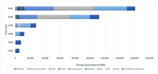
Figure 1.
Global direct primary energy consumption, 1800–2022. Direct primary energy consumption does not consider inefficiencies in fossil fuel production.
This is witnessed by the demand for energy worldwide falling significantly, especially in the first half of 2020. According to the International Energy Agency (IEA), there was an approximately 4% decrease in energy consumption in 2020 as compared to 2019 [8] when compared with the Australia market, which also experienced an overall energy consumption decrease around 4% in 2020 [9]. This is similar to the IEA figure; this highlights that the fall in commercial activity, industrial activity, and transportation as a result of lockdowns and restricted mobility has impacted overall energy consumption. In the period 2019–2020, Western Australia and the Northern Territory witnessed an increase in energy use, driven primarily by intensified energy consumption in the mining sector. However, the onset of COVID-19-related travel restrictions in March 2020 had a profound impact on energy consumption in the transportation sector in all states and territories. The scale of this decline varied across the country. New South Wales, the Northern Territory, and Victoria witnessed substantial reductions of more than 10% in energy consumption, while South Australia experienced a milder decline of 5%. Western Australia was a unique case, where a 1% growth in energy consumption was attributed to increased usage in metal ore mining, offset by declines in other sectors, especially transportation.
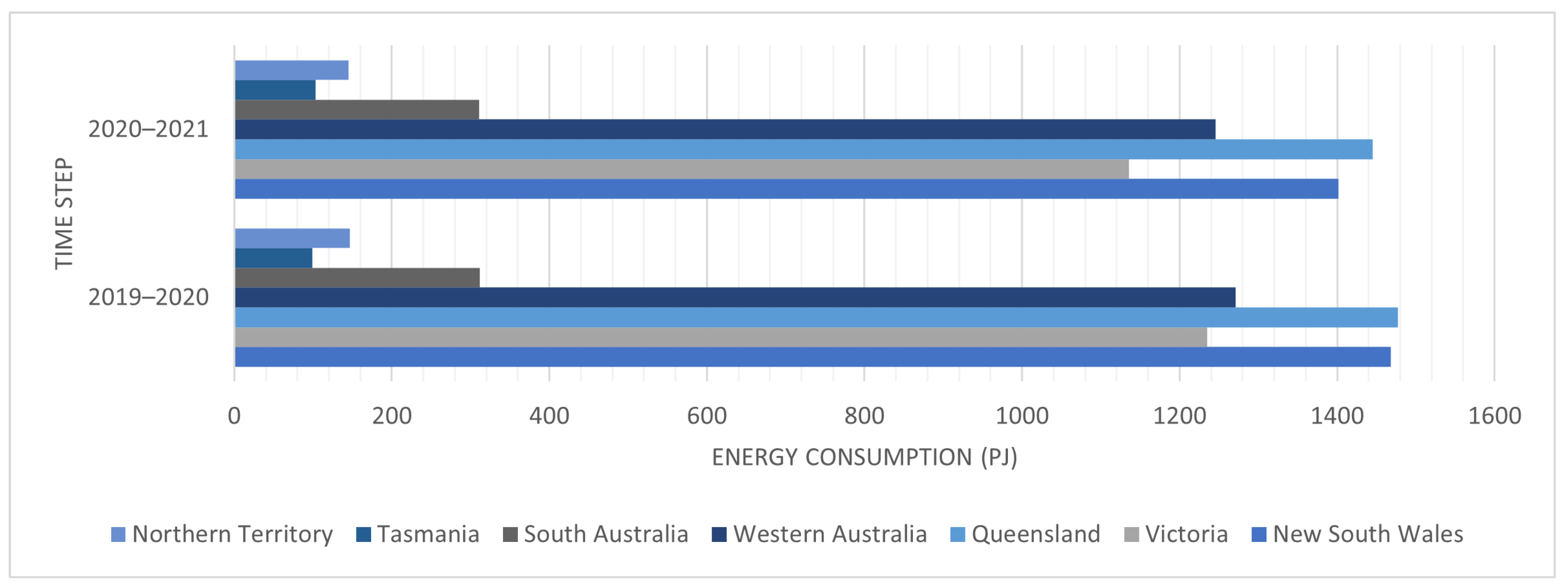
Of particular note are New South Wales and Victoria, which collectively accounted for nearly half of Australia’s energy consumption. These states recorded declines of approximately 5%, constituting more than 80% of the nationwide drop in energy consumption for the 2019–2020 period [10] (Figure 2). Fast forward to the 2020–2021 period, and the energy consumption landscape shifted. Queensland took the lead, representing approximately 25% of Australia’s total energy consumption, closely followed by New South Wales at approximately 24%. Western Australia and Victoria consumed approximately 22% and 20%, respectively. Tasmania, on the other hand, was the only state to observe an increase in energy consumption during this period, primarily due to a greater consumption of oil.

Figure 2.
Australian energy consumption, by state and territory, 2019–2021. New South Wales includes the Australian Capital Territory.
In contrast, Victoria’s energy consumption declined by 6%, while New South Wales experienced a 5% drop. The remaining states and territories saw reductions in energy consumption ranging from 1% to 3%, largely attributed to reduced activity resulting from the COVID-19 pandemic [11] (Figure 2).
A report tracking Victoria’s energy transition from 1989–1990 to 2019–2020 [12] shows notable changes in Victoria’s energy consumption or end-use of energy during this period. In the financial year 2019–2020, the total end use of energy in Victoria was 860.2 PJ. It was predominantly attributed to the transport sector (41.4%), followed by residential (21.3%), manufacturing (19%), and commercial (11.3%) sectors. However, the emergence of COVID-19 restrictions in the final four months of 2019–2020 disrupted these longstanding energy consumption patterns. Energy consumption decreased in the transport and commercial sectors, but it increased more than anticipated in the residential sector. This surge was due to factors such as increased remote work, limitations on travel distances and times, and restrictions on air travel. In the transition from 2018–2019 to 2019–2020, energy consumption in the residential sector showed a notable increase of 5.3%, but decreased by 10.8% in the transport sector and 4.4% in the commercial sector. The total Victorian electricity consumption in 2019–2020 was 174.0 PJ. The commercial sector was the main consumer of electricity (60.8 PJ, constituting 34.9% of the total), followed by residential (42.0 PJ, 24.1%), manufacturing (36.7 PJ, 21.1%), and electricity, gas, and water (24.6 PJ, 14.2%) sectors. Between 2018–2019 and 2019–2020, residential electricity consumption recorded a significant increase of 2.9 PJ (7.3%), and that in the electricity, gas, and water sectors jumped by 2.4 PJ (10.8%). On the contrary, commercial electricity consumption decreased by 2.5 PJ (4.0%). The alterations in energy usage underscore the importance of precise energy prediction. Forecasting of this nature is fundamental to enhancing the efficiency of resource distribution, enabling proficient energy administration, and bolstering the decision-making procedures of involved parties.
The implementation of lockdown measures on a global scale due to the COVID-19 pandemic has resulted in a discernible influence on the consumption of electricity across the globe. Numerous investigations have been carried out on the forecasting of energy, with particular focus on prediction during the COVID-19 pandemic in some of the studies [13,14,15]. Recent works have addressed uncertainties in data to minimize total expected energy costs [16] or to mitigate the impact of energy demand [17]. However, these studies do not directly focus on forecasting future demand in highly uncertain situations, such as those caused by the COVID-19 pandemic. Overall, the existing studies have tended to neglect the distinct challenges brought about by the pandemic, specifically within the realm of individual commercial structures, showing minimal focus on the meticulous monitoring of consumption trends at quarter-hourly intervals. Predicting building energy consumption at 15 min intervals offers several advantages. It provides detailed, high-resolution data on energy consumption, allowing a more precise understanding of usage patterns throughout the day. This level of prediction allows for almost real-time monitoring of energy consumption, enabling immediate responses to unusual spikes or drops in usage. It helps optimize building operations by identifying periods of high and low energy demand. This information can be used to schedule energy-intensive activities during off-peak hours, reducing costs.
Furthermore, during pandemic situation, it is necessary to incorporate noisy data to improve the robustness of forecasting models under unstable conditions. The concept of adversarial examples, which are specially crafted inputs, has gained prominence in the field of ensuring model reliability in order to enhance the robustness of models [18]. Adversarial examples are instances deliberately designed to cause a machine learning model to misbehave or produce incorrect predictions while appearing normal to human observers. These inputs are generated by introducing small, imperceptible perturbations into the original data, leading the model to make errors that would not occur in typical cases. However, despite its widespread application in various domains, the primary focus of adversarial examples has been predominantly restricted to the context of image processing. This emphasis on adversarial examples has not been equally extended to the realm of time-series forecasting, a crucial aspect in real-world applications, especially within domains such as energy consumption prediction. This disparity raises concerns about the reliability of models under volatile conditions, particularly during events such as the COVID-19 pandemic. Therefore, it becomes crucial to bolster the model’s resilience in such circumstances in order to cultivate greater user confidence when deploying these models in practical applications. In addition, a widely adopted approach to enhancing model robustness is adversarial training, which involves the direct introduction of adversarial noise into the training dataset, followed by model retraining aimed at improving accuracy. However, it is important to note that this strategy has been demonstrated to be inconsistent in terms of overall accuracy improvement and may, in fact, result in performance reductions for the original models [19].
This paper introduces a novel approach that aims to enhance the robustness of an energy consumption forecasting model through the integration of adversarial examples. We present a novel model, denoted , which builds on the foundation of as described by Tan et al. [20]. The latter is a multivariate long short-term memory model with knowledge integration specifically designed for COVID-19-related data. The main idea is that one incorporates adversarial example information by duplicating the energy information branch. In total, there are three branches in : (i) extraction of COVID-19 information; (ii) extraction of energy information; and (iii) extraction of adversarial energy information. Then, the outputs of the branches (ii) and (iii) are combined by average operation before concatenating the output of the branch (i) and forwarding to the prediction stage. Subsequently, the outputs from branches (ii) and (iii) are combined via an averaging operation before being concatenated with the output of branch (i) and subsequently fed into the prediction phase. In addition, we employ pre-trained models, including M-LSTM, long short-term memory (LSTM), bidirectional long short-term memory (Bi-LSTM), and Linear Regression (LR) models, which were originally presented in the research of Tan et al. [20]. We apply adversarial training, a common technique that involves the direct inclusion of adversarial examples in the training dataset and the fine-tuning of these pre-trained models. Subsequently, they are called adv-M-LSTM, adv-LSTM, adv-Bi-LSTM, and adv-LR. The experiment is carried out on three datasets on three commercial buildings with three common metrics: mean percentage absolute error (MAPE), normalized root mean squared error (NRMSE), and R-squared () metrics. The results show that the proposed model , closely matches the performance of in one dataset and surpasses other models in two additional datasets. This underscores the effectiveness of the proposed method in enhancing the robustness of energy consumption forecasting models, particularly amidst pandemic-related challenges. Overall, the proposed model significantly improves the accuracy of existing models in unstable situations.
2. Background
2.1. Energy Forecasting
This section presents a review of related literature, exploring the evolving landscape of energy consumption prediction amid the COVID-19 pandemic.
Abulibdeh et al. [14] employed machine learning methodologies and extensive empirical datasets to investigate the effects of the COVID-19 outbreak on electricity consumption and the precision of electricity demand forecasts within Qatari buildings. Their study spanned various sectors and timeframes, unveiling a correlation between the fluctuations in electricity consumption and the daily infection cases across specific socioeconomic domains. Shin et al. [15] examined the fluctuations in energy consumption within buildings in South Korea amidst the COVID-19 crisis, identifying the correlation between the pandemic and building energy utilization through an exploration of building usage patterns. Their findings highlight the general decline in energy consumption in most facilities in contrast to a surge in energy usage within residential spaces during the pandemic. Bourdeau et al. [21] conducted a review of studies that developed data-driven models to build scale applications. Runge et al. [22] presented a comprehensive review of research papers from the year 2000 that used artificial neural networks to predict building energy utilization and demand, with a particular focus on reviewing the applications, data, forecasting models, and performance metrics used in model evaluations. Focusing on the urban scale, Fathi et al. [23] delved into 70 journal articles published in the field of building energy performance forecasting between 2015 and 2018. Liu et al. [24] conducted a case study centered on an office building, employing three prevalent deep reinforcement learning techniques to forecast building energy consumption, namely, the asynchronous advantage actor-critic, the deep deterministic policy gradient, and the recurrent deterministic policy gradient methods. Somu et al. [25] introduced ’eDemand’, a robust energy consumption forecasting model that utilizes long short-term memory (LSTM) networks in conjunction with an enhanced sine-cosine optimization technique. Gassar et al. [26] provided a comprehensive overview of prevalent predictive methodologies employed in sizable building energy applications, embracing diverse scopes and archetypes ranging from black-box to white-box and gray-box approaches. Dong et al. [27] presented a prediction strategy for building energy consumption on the basis of ensemble learning and energy consumption pattern classification. In particular, human mobility data have emerged as a valuable asset within this domain, enabling the surveillance of occupancy patterns without the dependence on conventional sensors or manual data collection methods.
These studies offer predictive insights into and a comprehensive examination of the electricity landscape amid the COVID-19 pandemic. Table 1 presents an overview of various prediction models utilized for electricity consumption forecasting in commercial premises. Nonetheless, these analyses often disregard the unique hurdles presented by the pandemic, especially within the framework of commercial structures. To the best of the author’s knowledge, no prior studies have examined the precise impact of lockdown measures on the broad national electricity infrastructure, which is a critical consideration for sustaining secure and uninterrupted operations [28,29,30].

Table 1.
Overview of various prediction techniques for forecasting energy usage in commercial structures.
2.2. Robustness of AI Model
The robustness of AI models refers to the ability of a model to maintain its performance and accuracy under various conditions, including uncertainty, noise, etc. [39]. One of the main challenges to the robustness of AI is adversarial examples. The robustness of an AI model in adversarial settings refers to its ability to maintain consistent and accurate performance even when faced with deliberately crafted inputs designed to deceive or manipulate the model’s behavior. Adversarial settings involve scenarios where an attacker introduces modifications or perturbations to the input data, aiming to exploit vulnerabilities in the model’s decision-making process [40]. The robustness of models can be significantly enhanced through adversarial training, which enables the model to learn the characteristics of adversarial examples, as demonstrated. This training allows models to reliably predict values in noisy or unstable environments [18]. Additionally, defense strategies aim to develop neural networks that can resist adversarial examples, further reinforcing the reliability and accuracy of these models in adverse conditions [41].
Szegedy et al. [42] first discovered adversarial examples. They proved that small perturbations could decrease the confidence of an AI model. Inspired by this research, there have been a lot of subsequent studies focused on addressing the robustness of models in adversarial settings [18,41]. However, these studies predominantly centered on bolstering the robustness of image processing models, with comparatively less emphasis on sequence-based models [43] like time-series forecasting models.
The goal of enhancing robustness in AI models is to create systems that can provide reliable and trustworthy outputs, even in the presence of carefully crafted adversarial inputs. This ensures that the model’s performance remains consistent and accurate in real-world applications, bolstering its effectiveness and reliability in critical domains. Adversarial training is a popular approach to addressing this problem. That retrains the model with adversarial examples set to help the model achieve better accuracy in uncertain conditions. For instance, Wu et al. [44] demonstrate that adversarially trained models outperform standard models in predicting energy consumption during fluctuating energy usage patterns. However, this strategy often considerably affects the model’s accuracy under normal conditions [45].
3. Data Used in This Study
3.1. Data Collection
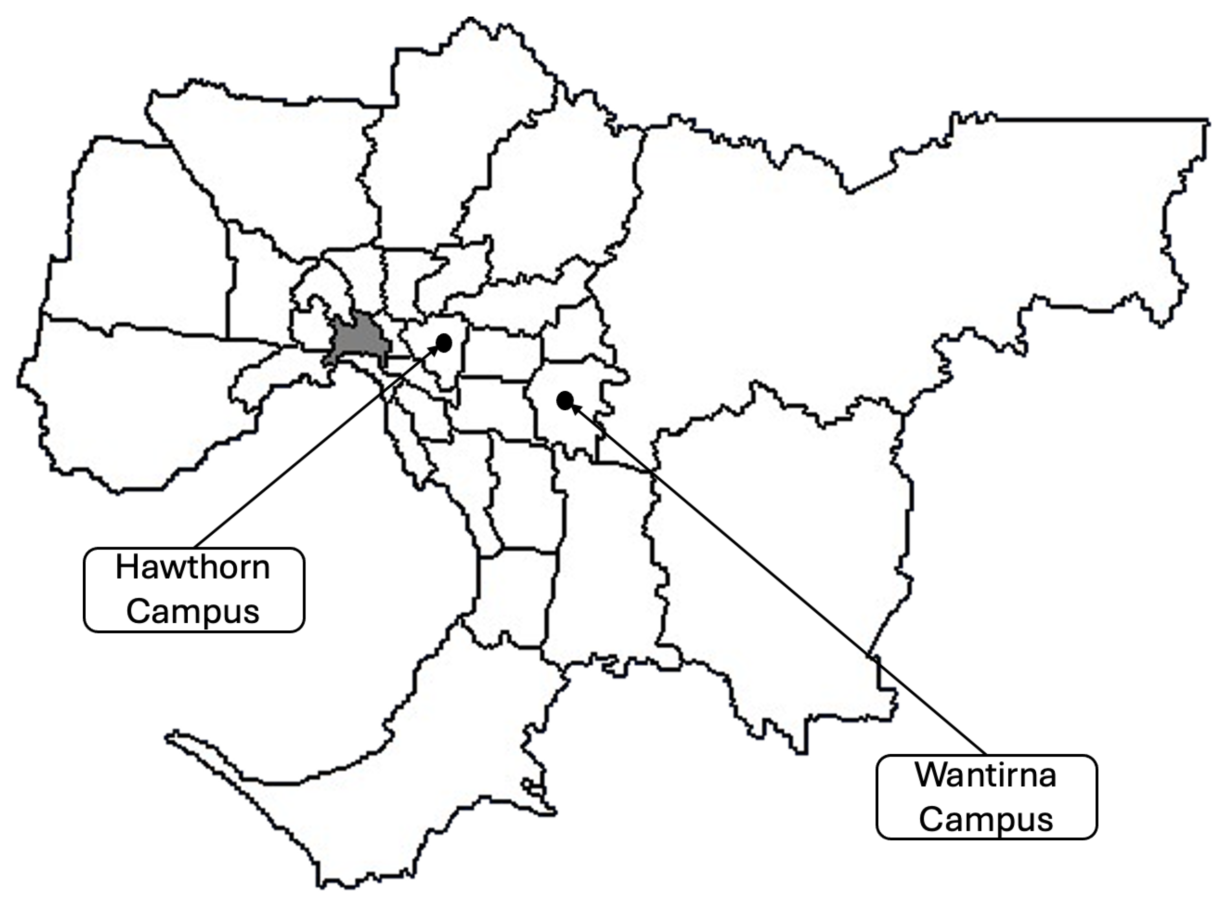
Utilizing data acquired from three distinct buildings across various geographical regions, namely Hawthorn Campus—ATC Building (referred to as 1), Hawthorn Campus—AMDC Building (referred to as 2), and Wantirna Campus—KIOSC Building (referred to as 3), prove immensely valuable Figure 3 [46]. This data stream provides immediate insights regarding the performance of buildings, patterns of energy consumption, and efficiencies in operations, facilitating prompt reactions to possible challenges. The utilization of real-time data plays a crucial role in enhancing decision-making proficiency within building management, maintenance, and optimization processes. Furthermore, it establishes a foundation for enhancing the precision of forecasting models. Moreover, it has the capacity to offer direction in strategic energy management, which may result in significant cost reductions, increased sustainability, and improved occupant comfort in the long run. The datasets 1, 2, and 3 encompass energy consumption records spanning from 2020 to 2021. The predictive value is derived from the discrepancy between previous and intermediate energy usage or cumulative energy consumption. The predictive process employs historical data encompassing 96 instances, each spanning a 15-min interval, to forecast the forthcoming value. The datasets from these three buildings enable accurate forecasting. It is suggested to provide real-time examples or instances where these data have led to precise insights.
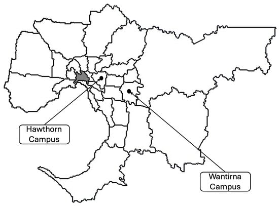
Figure 3.
The positioning of Hawthorn Campus and Wantirna Campus within Metropolitan Melbourne, Victoria, Australia.
3.2. Daily COVID-19 Cases in Victoria
Utilizing data obtained at 15 min intervals from three commercial buildings, we have amalgamated daily COVID-19 case data from Victoria in order to augment the precision of our predictive models. Victoria encountered several instances of stringent lockdown measures throughout the duration of the pandemic. The chronological sequence of these limitations is visually represented in Figure 4 [47], which illustrates daily COVID-19 case trends from February 2020 to January 2021. On 16 March 2020, a “state of emergency” was declared, initiating social distancing, remote work, and non-essential activity curbs [48]. Stricter measures at Stage 3 were implemented on 31 March 2020, subsequently alleviated on 13 May 2020, and further loosened on 1 June 2020.
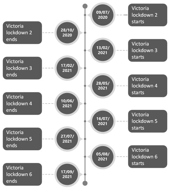
Figure 4.
Timeline of the Australia COVID-19 pandemic.
Nevertheless, as a result of an increase in COVID-19 infections and violations of hotel quarantine protocols, Stage 3 limitations were reimposed in Metropolitan Melbourne and Mitchell Shire. The second lockdown, termed “Vic lockdown 2”, commenced on 8 July 2020, following its announcement on 7 July 2020 [49]. A state of disaster was declared on 2 August 2020, enforcing Stage 4 restrictions in Metropolitan Melbourne for six weeks [50], later extending to 28 October 2020. When comparing the electrical demand from last year to the timeline of the Australia COVID-19 pandemic (Figure 4) during the “Vic lockdown 2” phase, according to the Australian Energy Regulator (AER), compared to the same months in 2019, Victoria’s power usage dropped by almost 10% during the lockdown period from July to October 2020. As many enterprises were either closing their doors or working at reduced capacity, a decline in industrial and commercial activity was a major factor in this loss. Residential power usage climbed as more individuals stayed at home as a result of lockdown measures, despite the overall drop. The drop in the commercial and industrial sectors was somewhat compensated by this increase in demand from homes. This is the same pattern when compared with the other major lockdown phases. These changes show the wider effects of COVID-19 on patterns of energy use, which are brought about by limitations on commercial activity and adjustments to work habits [51].
After an incident at the Holiday Inn, Victoria underwent an abrupt five-day period of restricted movement, officially known as “Vic lockdown 3”, spanning from 13 February to 17 February 2021, which involved a return to Stage 4 constraints [52]. Following this, Lockdown 4, a week-long circuit breaker lockdown, was enforced on 28 May 2021, in response to an outbreak, later extended until 10 June 2021 [53]. Subsequently, a swift five-day lockdown was enforced from 16 July to 20 July 2021 [52], initially, as Delta cases reached 18, extended until 27 July 2021 [54].
Just a little over a week following the relaxation of measures subsequent to the fifth period of enforced limitations, Victoria commenced its sixth period of enforced limitations on 5 August grappling with a surge in instances of the Delta variant. Announced initially for seven days, this lockdown was extended until 17 September 2021 [55]. Gradual relaxations of restrictions ensued, allowing for a semblance of normalcy to return. Despite this, localized lockdowns were imposed across states and territories in response to sporadic outbreaks, efficiently containing the virus. The momentum generated by the deployment of the vaccine instilled a sense of positivity regarding the times ahead. Towards the end of 2021, Australia transitioned from a policy of suppressing the virus to one of cohabitating with it, implementing a sophisticated method of imposing limitations that prioritizes the rate of vaccination, thereby laying the groundwork for a phase of recovery following the pandemic.
The COVID-19 pandemic has brought forth unparalleled and swiftly evolving conditions with profound ramifications for energy consumption trends. This has underscored the imperative of deploying robust data-driven models, like long short-term memory (LSTM), for predicting energy consumption. The global health crisis has initiated complex and evolving changes in energy consumption influenced by a variety of factors, including but not limited to restrictions on movement, the adoption of telecommuting, and fluctuations in the levels of industrial and commercial operations. LSTM, a type of recurrent neural network (RNN), has been intricately crafted to capture complex temporal associations and nonlinear patterns within data, thus proving to be proficient in both modeling and forecasting these dynamic fluctuations. By encompassing both immediate and prolonged interconnections within temporal data sequences, long short-term memory (LSTM) emerges as a crucial element in the landscape of the COVID-19 pandemic. This is particularly evident due to the concurrent impact of instant lockdown measures and the dynamic shifts towards remote work patterns on the consumption of energy. LSTM’s capacity to retain information across varying time spans equips it to handle such scenarios adeptly. Distinct from conventional neural networks, LSTM is characterized by its ability to propagate information from previous time steps to future ones through the process of backpropagation. The inherent characteristic of LSTM establishes it as a natural choice for the management of sequential data, such as the prediction of building loads. Studies, such as those by Zhang et al. [56] and Chen et al. [57], have shown that LSTM models outperform other time-series forecasting methods in predicting energy consumption during fluctuating periods and effectively capture non-linear relationships in energy data. The contemporary scenario, influenced by the COVID-19 pandemic, underscores the importance of employing data-centric models such as LSTM for forecasting energy consumption. This is mainly attributed to the model’s capacity to effectively manage intricate, dynamic, and ambiguous data patterns.
4. Methodology
4.1. Overview
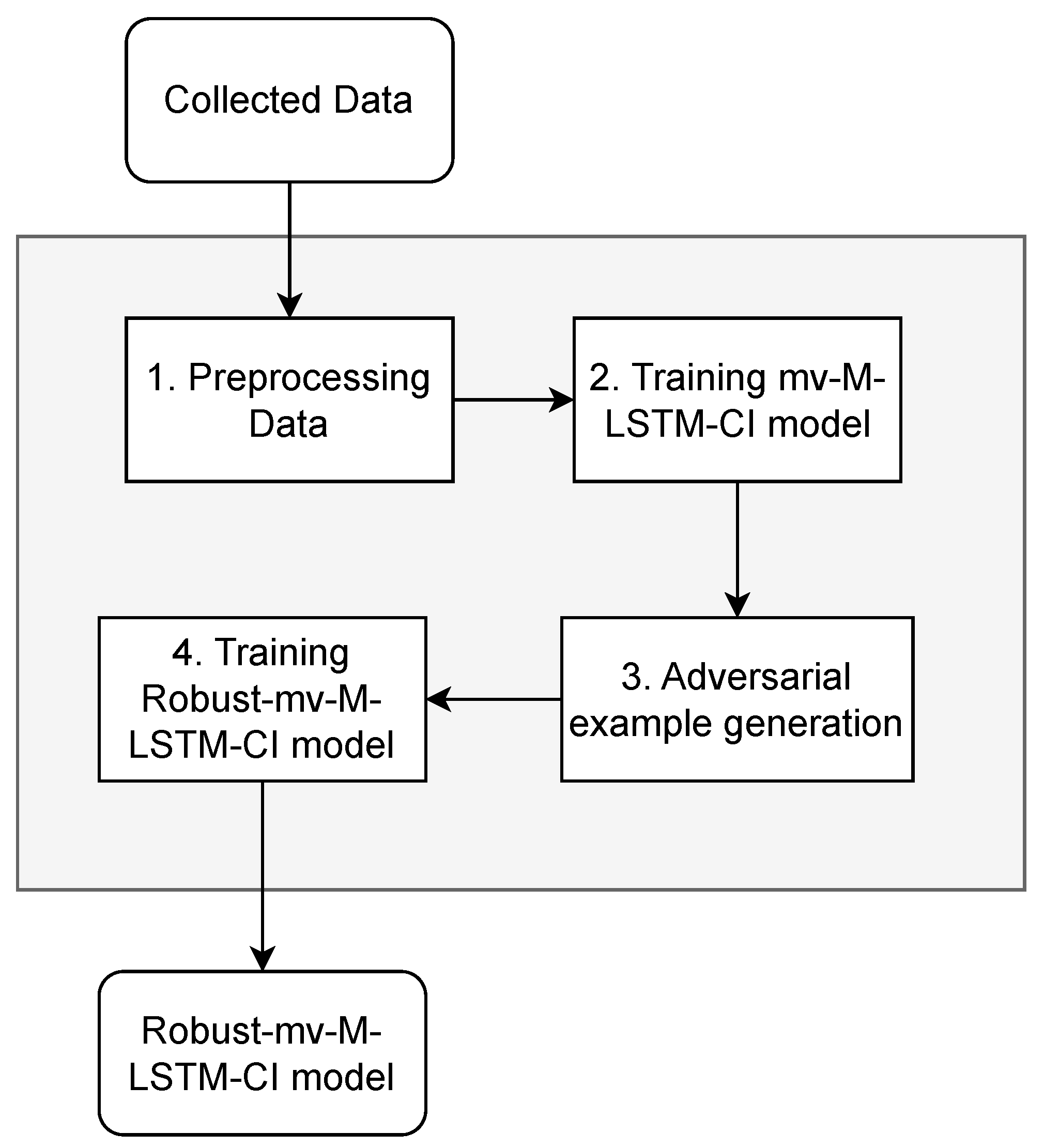
The schematic representation of the suggested approach is presented in Figure 5. The proposed model effectively learns from unstable data through specialized branches. It is designed to capture the unstable trend of the data during the pandemic. The knowledge gained from this branch is then integrated to make accurate predictions of future energy consumption during the pandemic. In particular, the input of the data collected from the commercial buildings. In this research, the data include the energy consumption in 15 min intervals, its timeline, and daily COVID-19 cases in the region. There are five main phases, i.e., 1. Preprocessing data (see Section 4.2), 2. Training model (see Section 4.3), 3. Generating adversarial example (see Section 4.4), and 4. Training model (see Section 4.5). The output of the proposed method is a trained, robust model with high accuracy in uncertain conditions.
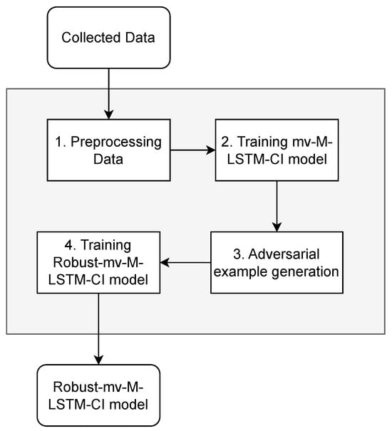
Figure 5.
The overall workflow of the proposed method.
4.2. Preprocessing Data
The data preprocessing phase is adapted from the research from Tan et al. [20]. This phase comprises two primary stages: (i) handling energy consumption and timeline, that is, the corresponding time in 15 min intervals, and (ii) managing COVID-19 data. Three fundamental types of input are present: a timeline, data on energy consumption, and daily occurrences of COVID-19. The term “timeline” denotes a sequence of time instances, each separated by 15-min intervals, establishing the chronological structure for the gathering and examination of data. Energy consumption quantifies the energy used within each 15-min interval, shedding light on energy usage patterns and fluctuations. Daily COVID-19 cases constitute the tally of COVID-19 incidents documented on a daily basis, offering a supplementary factor for examination and possible links with fluctuations in energy usage patterns.
The stage of handling energy consumption and timeline is composed of four steps: data differencing, time labeling, row concatenation, and window slicing. The process of data differencing encompasses the computation of variances between consecutive data points within a temporal sequence. By focusing on data point changes rather than raw values, the objective is to achieve stationarity in the data. Stationary data is generally more suitable for accurate modeling and prediction than dynamic data. The differencing energy consumption is denoted as 15. Analyzing peak and non-peak times can reveal underlying data trends. Understanding these patterns during distinct time frames allows for the identification of variations and the corresponding adjustments to forecasting models. In this study, the time span from 8:00 to 21:00 is categorized as peak hours, while the remaining hours are referred to as non-peak hours. The timeline at peak hour is labeled as 1, otherwise it is 0. The final vector of labeled time is denoted as 15.
During the phase of COVID-19 data management, the movement of individuals is often impacted by the number of COVID-19 cases throughout the COVID-19 period. Increased COVID-19 cases often lead to more stringent movement restrictions, especially when entering commercial establishments. Therefore, a reduction in energy consumption is typically observed within such structures. Therefore, Tan et al. [20] depicted the relationship between the total number of COVID-19 infections recorded in the previous two weeks and the consequent decrease in energy usage within commercial structures. They prove that integrating this data into forecasting models could enhance prediction accuracy. Thus, this subphase involves two key steps: the aggregation of COVID-19 cases and the normalization of the data. The aggregation of COVID-19 cases involves computing the total number of COVID-19 cases within the preceding 14 days, followed by restricting the data to a scale ranging from 0 to 10,000. The process of restricting the data, known as clipping, is executed to ensure that the data remains within a relevant range, thereby addressing any irregularities or extreme values that may influence the model’s performance. Through the process of rescaling values to a standardized range, the normalization of variations in COVID-19 case magnitudes is achieved, enabling equitable comparisons between different time periods and preventing any single feature from disproportionately influencing the learning process due to its scale. The normalization procedure is outlined in Equation (1).
where, signifies the accumulation of COVID-19 cases over the preceding 14 days for each time step , normalized to a scale between 0 and 1. The values and represent the uppermost and lowest extents of COVID-19 cases, correspondingly. The preprocessed COVID-19 data returned from this subphase is denoted as 19.
4.3. Training mv-M-LSTM-CI Model
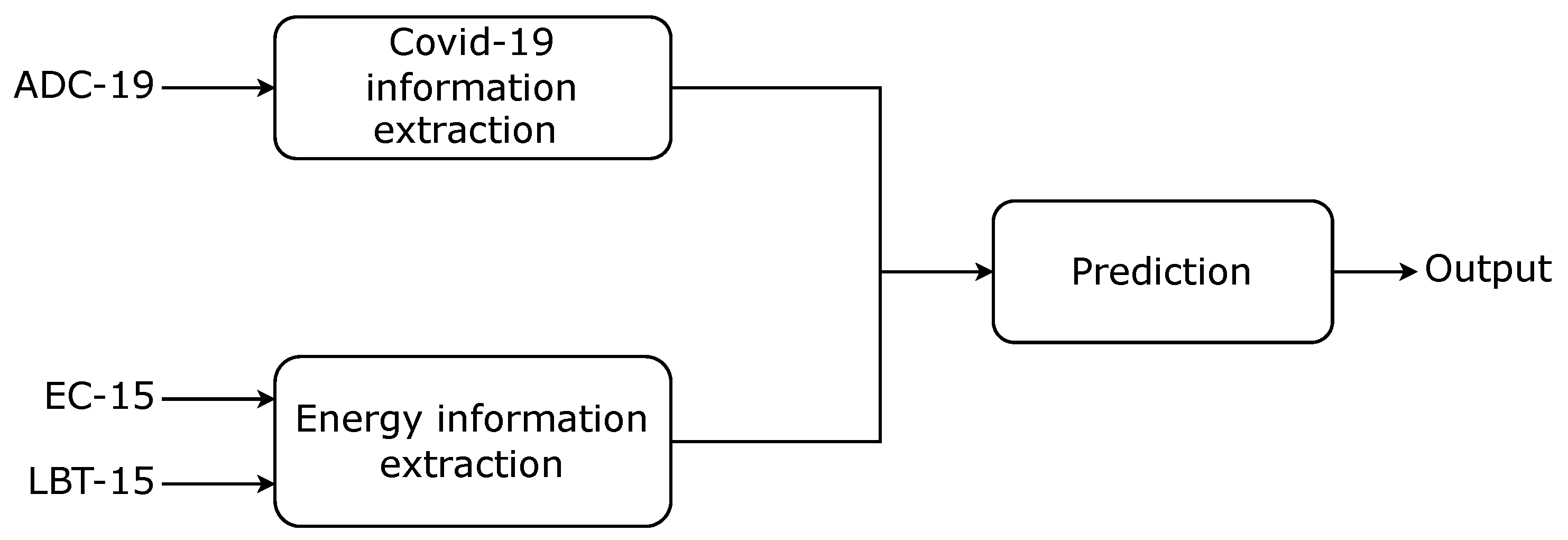
The model was originally proposed by Tan et al. [20]. It has been proven to outperform baseline models in all three datasets. In this study, plays an important role in training the proposed model. The is basically separated into three components: COVID-19 information extraction, energy information extraction, and prediction. The overall architecture of is shown in Figure 6.
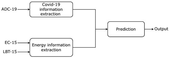
Figure 6.
Overview of model. 19: Accumulated Daily COVID-19 data, 15: Energy consumption in 15-min intervals, 15: labeled time in 15-min intervals.
The model features two input streams: one for energy consumption and labeled time, and the other for normalized COVID-19 data. The first stream employs a specialized multivariate LSTM architecture with two consecutive LSTM layers. These layers capture temporal patterns within energy consumption data. Each LSTM cell consists of input, forget, and output gates, governing information flow. An update function regulated by a function maintains information passage. Cell and hidden states are generated per cell calculation.
In the second stream, COVID-19 data undergoes a dense layer for insightful extraction. The dense output combines with the last hidden state of the second LSTM layer, injecting knowledge. The outputs from both streams concatenate, merging LSTM-derived representations with COVID-19 insights. This combination proceeds through dense layers and batch normalization to yield the final decision.
Huber loss serves as the objective function for model training. It balances mean absolute and mean squared errors and accommodates extreme values and anomalous events.
where the loss function’s parameter determines the transition between quadratic and linear loss regions, and are actual and predicted value for input , respectively. However, the robustness of the model should be further improved with perturbed input for a better accuracy under unstable conditions.
4.4. Generating Adversarial Example
The aim of this phase is to generate adversarial examples for training the proposed model. Commonly, adversarial examples are crafted with the intent to deceive models. While engineers emphasize model correctness, focusing on accuracy, loss on dataset, and similar metrics, they often overlook the robustness of the model. Consequently, models that perform well under normal circumstances might exhibit incorrect behavior in abnormal situations [39]. For example, AI models in self-driving cars can accurately recognize and classify objects like pedestrians, other vehicles, and traffic signs under normal conditions with clear weather and good lighting.Attackers could place subtle stickers or graffiti on stop signs that the human eye would still recognize as a stop sign, but the AI model might misclassify it as a yield sign or ignore it altogether [58]. These values help predict real-time scenarios by reflecting model sensitivity to minor input changes, thereby enhancing robustness through adversarial training. This aspect, to our knowledge, remains relatively unexplored in the context of time-series forecasting for energy consumption.
This study addresses this gap by integrating adversarial examples to enhance the robustness of forecasting models. Specifically, we employ noisy adversarial examples, generated through the Fast Gradient Sign Method (FGSM) introduced by Ian J. Goodfellow et al. [59]. The Huber loss of model (abbreviated as ) is defined using a threshold (Equation (2)). The noise for the original energy consumption input in the FGSM method is derived as the gradient of the loss function of with respect to each individual input (Equation (3)).
This gradient-derived noise perturbs the legitimate input , leading to the creation of an adversarial example (Equation (4)). Here, regulates the extent of noise introduced, constrained by the distance to be within .
where is to control the amount of noise needed to perturb with the maximum noise must be less than in terms of distance as shown in Equation (5).
In this research, we generate a set of adversaries with a maximum noise of 0.005, ensuring minimal changes to the original input set across the three datasets studied. Notably, is set to 1. For 1, 2, and 3, in terms of average distance for all energy consumption inputs, the average noise levels are 2.29 , 3.50 , and 2.24 , respectively. Although these values are minute to maintain real-world validity, they yield substantial enhancements in model performance.
4.5. Robust-mv-M-LSTM-CI Model
In this paper, we propose an enhanced version of this model. The proposed model is called .
As mentioned, the is basically separated into three components: COVID-19 information extraction, energy information extraction, and prediction. While adversarial training has emerged as a popular means to bolster model robustness, it often comes at the cost of compromising the model’s primary performance [40]. Addressing this limitation, this study introduces an architecture that not only preserves the model’s original performance but also enhances accuracy within noisy contexts.
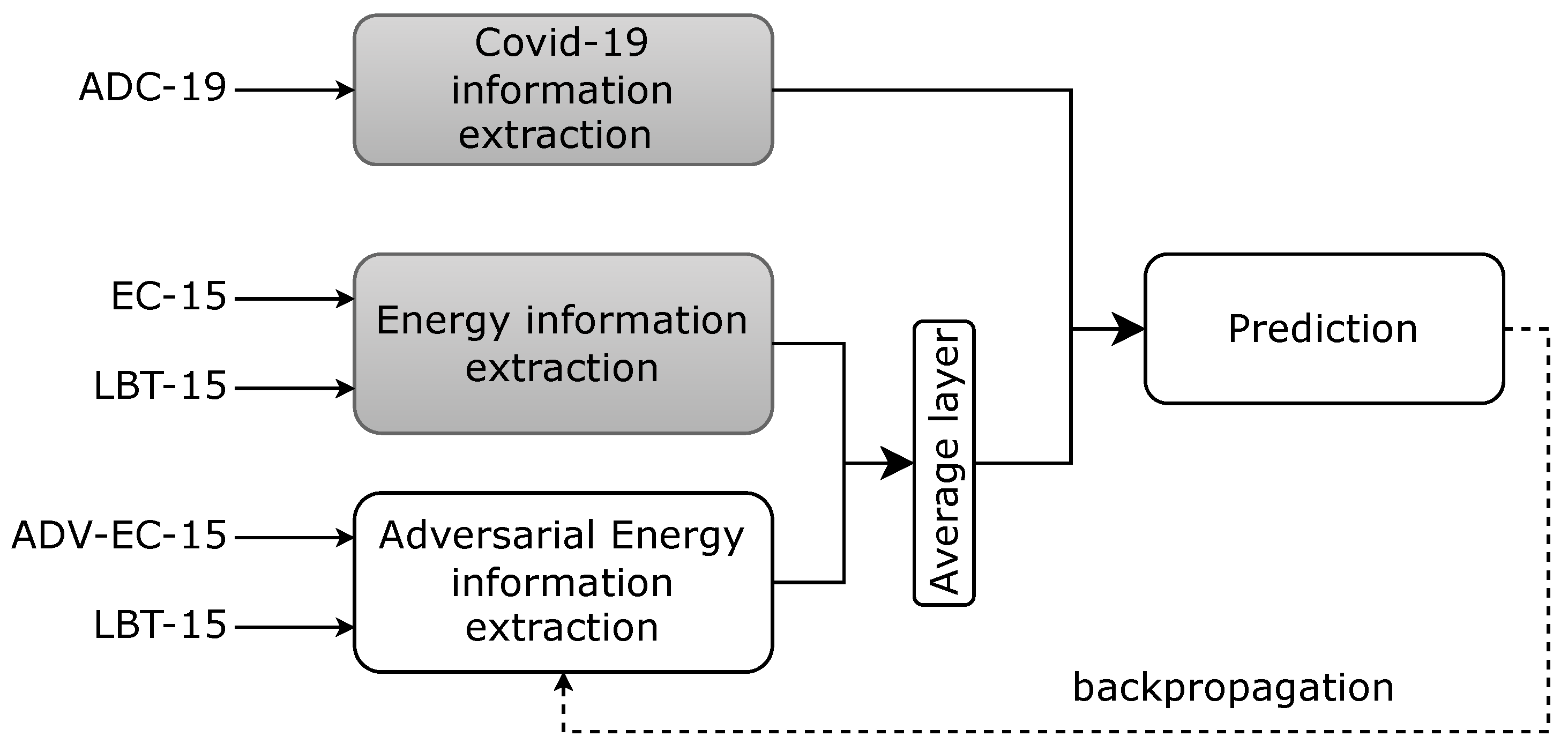
The overview architecture of is shown in Figure 7. In this model, we create one block called adversarial energy information extraction. The input is an adversarial dataset (referred to as 15) and the labeled time in 15-min intervals. Initially, this block duplicates from the energy information extraction all related information such as architecture, weights, etc. There is an average layer that takes the output from energy information extraction blocks () and its adversarial blocks () for enhancing the model in noisy conditions. In particular, the output of this layer is computed as Equation (6).
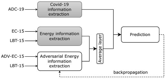
Figure 7.
The overall training workflow of model. The gray block indicates that they freeze.
In the training process, the COVID-19 information extraction and energy information extraction blocks are frozen to preserve their original ability. The adversarial energy information extraction is trained to inherit the energy information and capture the noisy information with adversarial energy consumption and labeled time within 15 min. The output is averaged with the original energy information before being used to finetune the prediction stage. The loss is kept the same as the loss of .
In general, the designed data preprocessing, architecture of the model, and training strategy aim to improve the robustness of the trained model in a noisy environment. In addition, they do not affect the original model.
5. Baseline Models
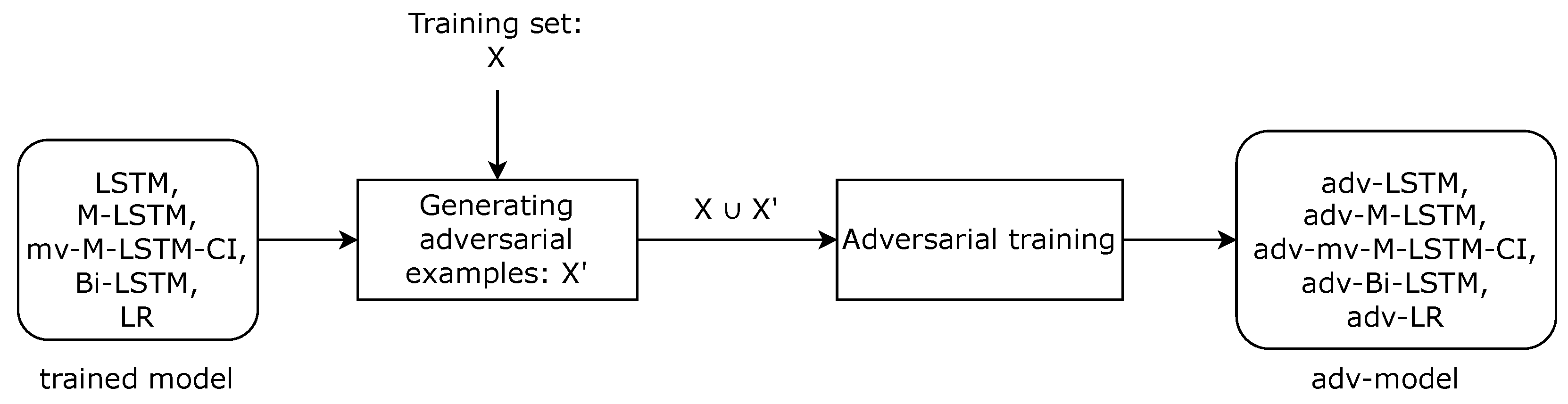
In this research, the proposed model is compared with the base model: and adversarial training of trained models from our previous research [20]: multivariate multilayered long short-term memory (M-LSTM), long short-term memory (LSTM), bidirectional long short-term memory (Bi-LSTM), and linear regression (LR). As shown in Figure 8, adversarial training comprises two primary phases. In the first phase, an adversarial examples set () is generated using trained forecasting models and the original training dataset (), which were previously established in our prior research [20]. This process results in an augmented training dataset (). In the second phase, the trained models undergo further training using the expanded training dataset, leading to the final models labeled with the prefix “adv-”. Note that the model architectures are kept as its origins. The details of these models are described as follows:

Figure 8.
The process of adversarial training in baseline models.
adv-LSTM: This model is obtained from the LSTM model with a single LSTM layer through adversarial training. This is a specialized recurrent neural network architecture known for its ability to capture and retain long-range dependencies in sequential energy consumption. In the adversarial generation, the average noise levels for 1, 2, and 3 are 3.84 , 1.30 , and 1.43 , respectively.
Adv-M-LSTM: This model is obtained from M-LSTM [46] model through adversarial training, a multivariate multilayer LSTM model with one follow to process energy consumption information with labeled time to predict future energy consumption. In the adversarial generation, the average noise levels for 1, 2, and 3 are 4.80 , 2.40 , and 2.03 , respectively.
: This model is obtained from through adversarial training. is a multivariate LSTM model with two branches: energy information extraction and COVID-19 information extraction for forecasting energy usage during COVID-19 pandemic. In the adversarial generation, the average noise levels for 1, 2, and 3 are 2.29 , 3.50 , and 2.24 , respectively. These numbers are similar to the noise described in Section 4.4.
adv-Bi-LSTM: This model is obtained from the Bi-LSTM model through adversarial training. Bi-LSTM is a variant of the LSTM architecture that processes input sequences in both forward and backward directions simultaneously. This dual processing capability enables it to capture contextual information from past and future energy consumption. In the adversarial generation, the average noise levels for 1, 2, and 3 are 1.44 , 3.20 , and 3.97 , respectively.
adv-LR: This model is obtained from the LR model through adversarial training. LR is employed to establish relationships between historical energy consumption and future consumption. This model is simple and effective when there is a linear relationship between variables. In the adversarial generation, the average noise levels for 1, 2, and 3 are 0.99 , 1.33 , and 0.50 , respectively.
6. Experiment
This experiment is carried out to exhibit the effectiveness of the proposed model in comparison to the baseline models, namely and , and “adv-” models as described in Section 5. Three distinct datasets are employed: Hawthorn Campus—ATC Building (referred to as 1), Hawthorn Campus—AMDC Building (referred to as 2), and Wantirna Campus—KIOSC Building (referred to as 3).
6.1. Metric
The evaluation is based on three key metrics: mean absolute percentage error (MAPE), normalized mean square error (NMSE), and the score. After training, the models generate predictions, which are then compared with the actual values using these metrics. This comparison helps assess each model’s performance and facilitates benchmarking against other models.
MAPE. The calculation of MAPE involves determining the absolute discrepancy between the forecasted and observed figures, succeeded by a process of dividing by the observed value. This process is repeated for all data points, and the resulting values are averaged across the dataset, as shown in Equation (7). This computation yields a solitary numerical value indicating the average percentage disparity between predictions and actual values. A lower MAPE value indicates superior model performance, as it signifies a reduced average percentage deviation between predictions () and actual values (), with the total number of instances being .
NRMSE: The NRMSE is a performance metric utilized to assess the accuracy of a prediction model. This metric gauges the normalized average size of the discrepancies or discrepancies between projected and observed values, as elucidated in Equation (8). By taking the square root of the mean square errors (MSEs) and standardizing them, the NRMSE offers an assessment of the general disparity between predicted and actual values while accounting for the data’s magnitude, with are maximum and minimum values of actual values , respectively. A lower NRMSE value reflects the strong alignment of the model with the data, signifying heightened accuracy in predictions.
score. The score, denoted as the coefficient of determination, serves as a statistical metric that measures the extent to which the variance in the dependent variable can be explained by the predictor variables in a regression framework, as depicted in Equation (9). The value denotes the mean of the observed values and indicates the model’s appropriateness and capacity to accurately predict the target outcome. A high score denotes a favorable alignment of the model, suggesting that a significant proportion of the variance in the dependent variable can be ascribed to the predictor variables.
6.2. Results and Discussion
Table 2 presents a comprehensive insight into the performance evaluation of various models across three distinct datasets.
Table 2.
Evaluation of forecasting models based on three metrics across three datasets. Optimal values are bold for emphasis.
In 1, showcases its accuracy with an MPAE of 0.062 and an NRMSE of 0.049. These results, while strong, are slightly higher than those of its origin, , which records an MPAE of 0.061 and an NRMSE of 0.047. In detail, exhibited a slight increase in mean percentage absolute error (MPAE) of approximately 1.64% compared to . In NRMSE, displayed a minor increase of around 4.26%. It registered a marginal decrease of roughly 0.54% in score. However, it is essential to note that the difference is relatively minor. This difference is acceptable while considering the performance in 2 and 3. On the other hand, exhibited a more substantial decrease in performance with an MPAE increase of about 94.26%, an NRMSE increase of approximately 73.19%, and a substantial decrease in score by approximately 15.25%. In addition, in this dataset, delivers competitive performance, demonstrating its resilience and capacity to handle challenging scenarios. Moreover, it outperforms other adversarially trained models, including Adv-M-LSTM, Adv-LSTM, Adv-BiLSTM, and Adv-LR underscoring its enhanced accuracy and reliability.
In 2, demonstrates its remarkable performance with an MPAE of 0.065, NRMSE of 0.042, and an score of 0.878. This reflects an impressive improvement over the original model, , by approximately 30% in MPAE, 32% in NRMSE, and around 4.5% in score. Such notable enhancements underscore the robustness of while maintaining the high accuracy standards set by . When compared to other adversarially trained models, it significantly outperforms them, highlighting its potential for precise energy consumption forecasting even in challenging conditions.
Moving to 3, consistently outshines with an MPAE of 0.087, an NRMSE of 0.024, and an impressive score of 0.945. Here, showcases a substantial improvement over with a remarkable percentage improvement of approximately 45% in MPAE, 27% in NRMSE, and roughly 5.6% in score. These findings emphasize the model’s robustness while substantially improving accuracy compared to the baseline. The proposed model consistently outperforms other adversarially trained models, confirming its capability to provide highly accurate energy consumption forecasts, even in demanding scenarios.
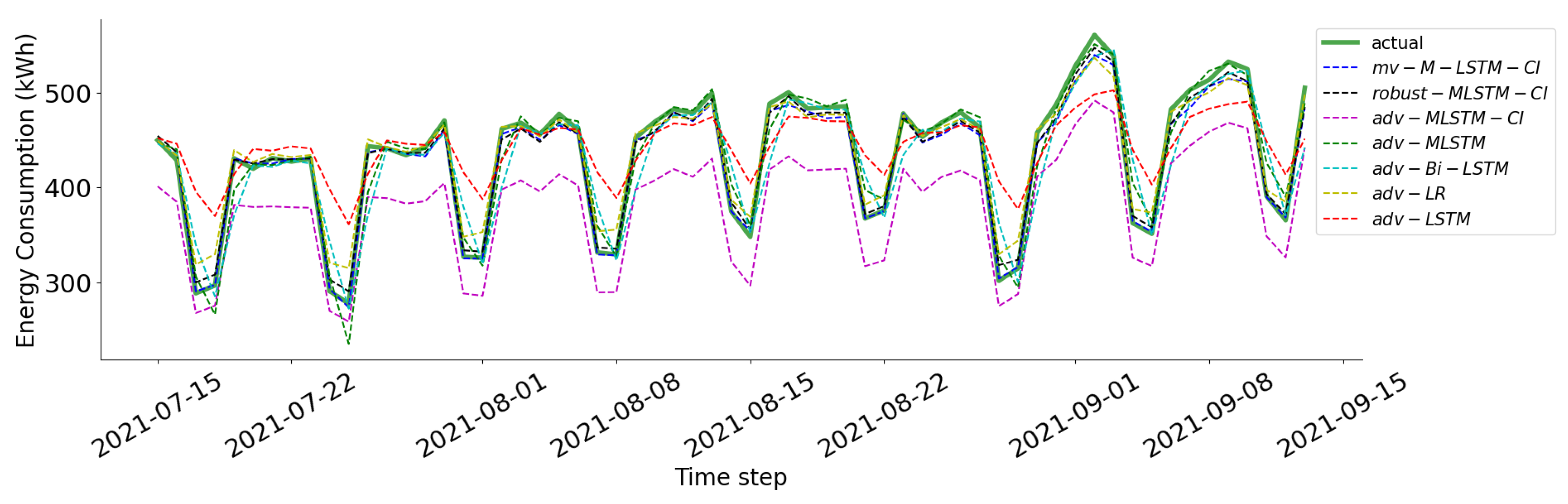
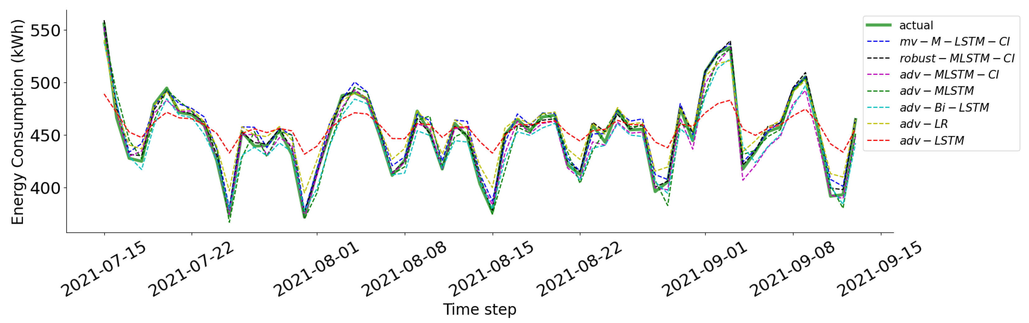
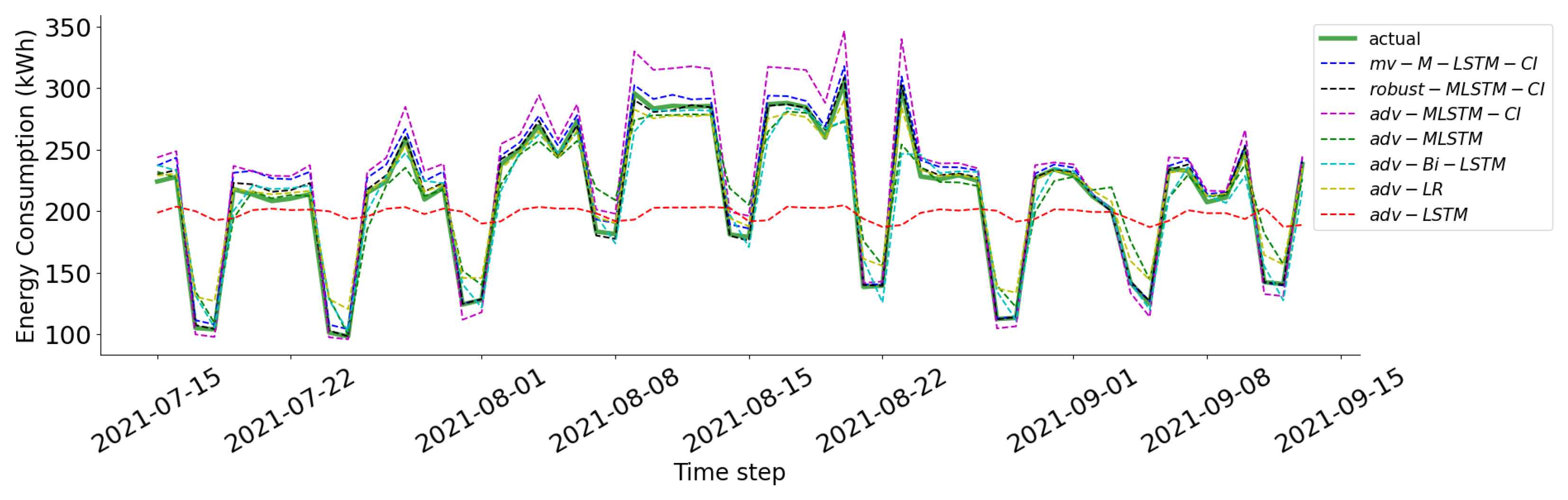
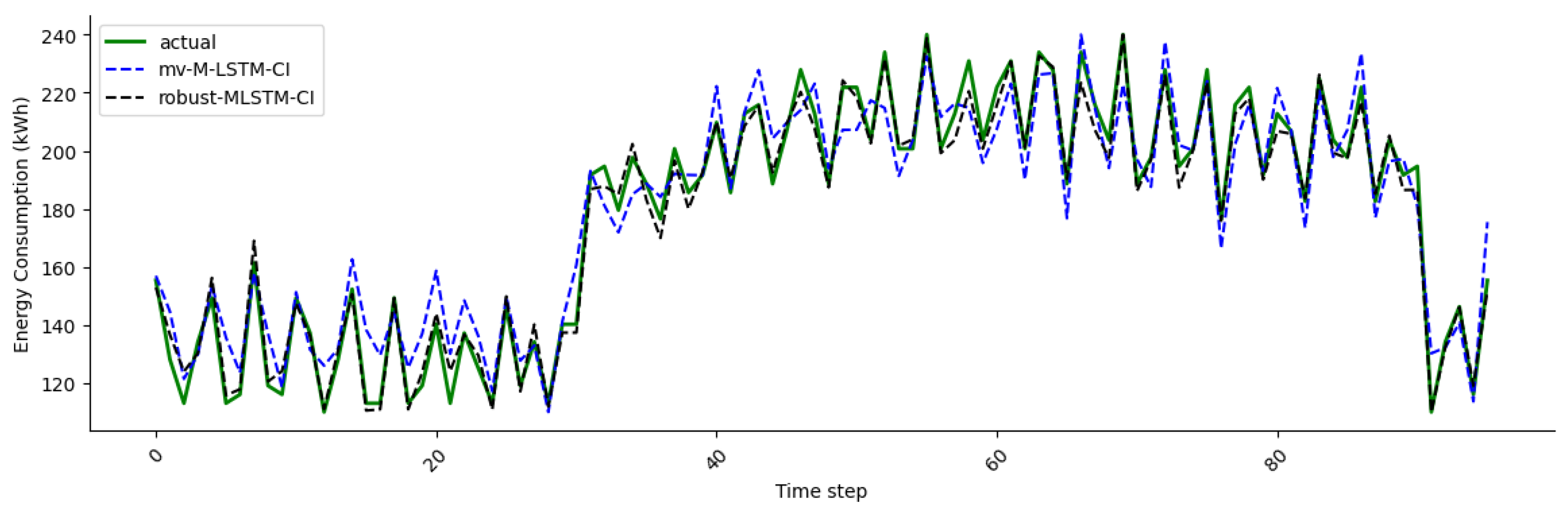
Furthermore, to enhance the clarity of visual representation, Figure 9, Figure 10, Figure 11 and Figure 12 depict the performance of the forecasting models spanning from 15 July 2021 to 15 September 2021. For better visualization, Figure 4 presents a zoomed-in view of every 15 min for a day from 17 July to 18 July 2021 on 3, comparing the two best-performing models, and . This detailed examination highlights their predictive accuracy over this specific period. These figures offer insights into the model’s performance trends over this time period. In a broad sense, the graphs distinctly portray that the proposed model consistently maintains a good fit when compared to the alternative models. However, it is noteworthy that the accuracy of the experiences a significant degradation, evident from its performance on the test sets.
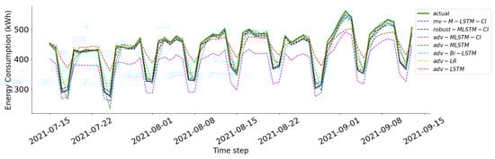
Figure 9.
Prediction for energy consumption every day of forecasting models on 1.
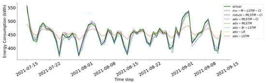
Figure 10.
Prediction for energy consumption every day of forecasting models on 2.
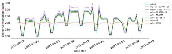
Figure 11.
Prediction for energy consumption every day of forecasting models on 3.

Figure 12.
The detail on prediction of and from 17 July and 18 July 2021.
Overall, the results highlight the consistent superiority of the proposed model across all three datasets. Its ability to minimize prediction errors and explain a higher proportion of variability positions it as a robust and accurate choice for time-series forecasting tasks. Furthermore, the results also reveal that the conventional adversarial training approach may lead to a decline in the performance of the original models.
7. Conclusions
In essence, this manuscript introduces an innovative predictive model with an adaptable design, designed for potential adjustments in forthcoming epidemic outbreaks and analogous emergency circumstances. The main idea is that the proposed method incorporates adversarial examples generated from the model by adding a new branch to process input with adversarial noise. Our research was centered on forecasting energy usage in three separate structures situated at the Hawthorn and Wantirna campuses: 1, 2, and 3. The experimental results demonstrate that the proposed model outperforms baseline models, including , conventional adversarial training models: , adv-M-LSTM, adv-LSTM, adv-Bi-LSTM, and adv-LR with three widely-used metrics: MAPE, NRMSE, and score. The results show that:
- In 1, achieved an MPAE of 0.062 and an NRMSE of 0.049, slightly higher than ’s MPAE of 0.061 and NRMSE of 0.047. Despite minor increases in error rates and a slight decrease in the score, the proposed model remains competitive and outperforms other adversarially trained models.
- In 2, showed superior performance with an MPAE of 0.065, NRMSE of 0.042, and an score of 0.878, improving significantly over . These results demonstrate ’s robustness and higher accuracy, outperforming other adversarially trained models.
- In 3, excelled with an MPAE of 0.087, NRMSE of 0.024, and score of 0.945, showing substantial improvements over . This highlights the model’s robustness and enhanced accuracy, consistently outperforming other adversarially trained models.
Our findings shed light on the potential limitations of adversarial training, which, when directly integrated into the energy consumption processing branch, may compromise the overall accuracy of the original model. However, by introducing a dedicated branch tailored for the processing of adversarial noise, the proposed model effectively bolsters accuracy, surpassing other “adv-” models across three datasets. The proposed model carries significant implications for efficient energy management and conservation within academic buildings. The versatility of this methodology may have the capacity to be applied to comparable educational establishments exhibiting similar energy usage trends, providing a beneficial resolution for energy governance within the academic sphere.
In the future, there is potential to explore how the proposed model can be tailored to different architectural frameworks, such as combinations of various architectures and heightened complexity levels. This exploration aims to pinpoint the optimal configuration for precise energy forecasting within specific scenarios. This could seek to identify the most suitable configuration for each specific energy forecasting scenario. In addition, in order to maximize the utility of the proposed model, it is worth considering experiments with datasets representative of diverse real-world conditions. This approach can facilitate broader applications of the model in energy forecasting for buildings.
Author Contributions
Individual Contribution: Conceptualization, T.N.D., G.S.T., M.S., S.M. and A.S.; Methodology, T.N.D., G.S.T. and M.S.; Software, T.N.D. and G.S.T.; Validation, M.S., A.S. and S.M.; Formal analysis, G.S.T., M.S., A.S. and S.M.; Investigation, G.S.T., M.S., S.M. and A.S.; Resources, M.S., A.S. and S.M.; Data curation, G.S.T., T.N.D. and M.S.; Writing-original draft preparation, T.N.D. and G.S.T.; Writing-review and Editing, M.S., S.M. and A.S.; Visualization, G.S.T., T.N.D. and M.S. All authors have read and agreed to the published version of the manuscript.
Funding
This research received no external funding.
Institutional Review Board Statement
Not applicable.
Informed Consent Statement
Not applicable.
Data Availability Statement
The data presented in this study are available on request from the corresponding author.
Conflicts of Interest
The authors declare no conflicts of interest.
References
- Sadigov, R. Rapid growth of the world population and its socioeconomic results. Sci. World J. 2022, 2022, 8110229. [Google Scholar] [CrossRef] [PubMed]
- Online Global Direct Primary Energy Consumption. Available online: https://ourworldindata.org/grapher/global-primary-energy (accessed on 8 November 2023).
- Online Buildings. Available online: https://www.iea.org/energy-system/buildings (accessed on 8 November 2023).
- Online Commercial Buildings Energy Consumption Baseline Study 2022. Available online: https://www.energy.gov.au/publications/commercial-buildings-energy-consumption-baseline-study-2022 (accessed on 8 November 2023).
- Online Electricity Prices Fall and COVID Spikes Residential Demand. Available online: https://www.accc.gov.au/media-release/electricity-prices-fall-and-covid-spikes-residential-demand (accessed on 8 November 2023).
- Online Working from Home’s Impact on Electricity Use in the Pandemic. Available online: https://www.nber.org/digest/202012/working-homes-impact-electricity-use-pandemic (accessed on 8 November 2023).
- Online Speed and Surprises: Decline and Recovery of Global Electricity Use in COVID’s First Seven Months. Available online: https://news.stanford.edu/2022/02/11/fall-rise-electricity-use-early-pandemic/ (accessed on 8 November 2023).
- IEA. Global Energy Review 2021—Analysis. 2021. Available online: https://www.iea.org/reports/global-energy-review-2021 (accessed on 18 July 2024).
- Grozinger, P.; Parsons, S. The COVID-19 Outbreak and Australia’s Education and Tourism Exports, Bulletin—December Quarter. Bulletin. 2020. Available online: https://www.rba.gov.au/publications/bulletin/2020/dec/the-covid-19-outbreak-and-australias-education-and-tourism-exports.html (accessed on 18 July 2024).
- Australian Energy Update 2021. Available online: https://www.energy.gov.au/publications/australian-energy-update-2021 (accessed on 17 May 2023).
- States and Territories. Available online: https://www.energy.gov.au/data/states-and-territories (accessed on 1 September 2023).
- Tracking Victoria’s Energy Transition 2020. Available online: https://www.sustainability.vic.gov.au/research-data-and-insights/research/research-reports/tracking-victorias-energy-transition-2020 (accessed on 1 September 2023).
- Jogunola, O.; Morley, C.; Akpan, I.J.; Tsado, Y.; Adebisi, B.; Yao, L. En-ergy Consumption in Commercial Buildings in a Post-COVID-19 World. IEEE Eng. Manag. Rev. 2022, 50, 54–64. [Google Scholar] [CrossRef]
- Abulibdeh, A.; Zaidan, E.; Jabbar, R. The impact of COVID-19 pandemic on electricity consumption and electricity demand forecasting accuracy: Empirical evidence from the state of Qatar. Energy Strategy Rev. 2022, 44, 100980. [Google Scholar] [CrossRef]
- Hosseini, S.M.; Carli, R.; Dotoli, M. Robust Optimal Demand Response of Energy-efficient Commercial Buildings. In Proceedings of the 2022 European Control Conference (ECC), London, UK, 12–15 July 2022; pp. 1–6. [Google Scholar] [CrossRef]
- Shin, S.-Y.; Woo, H.-G. Energy Consumption Forecasting in Korea Using Machine Learning Algorithms. Energies 2022, 15, 4880. [Google Scholar] [CrossRef]
- Di Piazza, M.C.; La Tona, G.; Luna, M.; Di Piazza, A. A two-stage Energy Management System for smart buildings reducing the impact of demand uncertainty. Energy Build. 2017, 139, 1–9. [Google Scholar] [CrossRef]
- Aldahdooh, A.; Hamidouche, W.; Fezza, S.A.; Déforges, O. Adversarial example detection for DNN models: A review and experimental comparison. Artif. Intell. Rev. 2022, 55, 4403–4462. [Google Scholar] [CrossRef]
- Bai, T.; Luo, J.; Zhao, J.; Wen, B.; Wang, Q. Recent Advances in Adversarial Training for Adversarial Robustness. In Proceedings of the Thirtieth International Joint Conference on Artificial Intelligence (IJCAI-21), Montreal, QC, Canda, 19–27 August 2021; pp. 4312–4321. [Google Scholar] [CrossRef]
- Dinh, T.; Thirunavukkarasu, G.; Seyedmahmoudian, M.; Mekhilef, S.; Stojcevski, A. Energy Consumption Forecasting in Commercial Buildings during the COVID-19 Pandemic: A Multivariate Multilayered Long-Short Term Memory Time-series Model with Knowledge Injection. Sustainability 2023, 15, 12951. [Google Scholar] [CrossRef]
- Bourdeau, M.; Zhai, X.; Nefzaoui, E.; Guo, X.; Chatellier, P. Modeling and forecasting building energy consumption: A review of data-driven techniques. Sustain. Cities Soc. 2019, 48, 101533. [Google Scholar] [CrossRef]
- Runge, J.; Zmeureanu, R. Forecasting Energy Use in Buildings Using Artificial Neural Networks: A Review. Energies 2019, 12, 3254. [Google Scholar] [CrossRef]
- Fathi, S.; Srinivasan, R.; Fenner, A.; Fathi, S. Machine learning applications in urban building energy performance forecasting: A systematic review. Renew. Sustain. Energy Rev. 2020, 133, 110287. [Google Scholar] [CrossRef]
- Liu, T.; Tan, Z.; Xu, C.; Chen, H.; Li, Z. Study on deep reinforcement learning techniques for building energy consumption forecasting. Energy Build. 2020, 208, 109675. [Google Scholar] [CrossRef]
- Somu, N.; Raman, M.G.; Ramamritham, K. A hybrid model for building energy consumption forecasting using long short term memory networks. Appl. Energy 2020, 261, 114131. [Google Scholar] [CrossRef]
- Gassar, A.A.A.; Cha, S.H. Energy prediction techniques for large-scale buildings towards a sustainable built environment: A review. Energy Build. 2020, 224, 110238. [Google Scholar] [CrossRef]
- Dong, Z.; Liu, J.; Liu, B.; Li, K.; Li, X. Hourly energy consumption prediction of an office building based on ensemble learning and energy consumption pattern classification. Energy Build. 2021, 241, 110929. [Google Scholar] [CrossRef]
- AEMO. Quarterly Energy Dynamics Q2 2020 Market Insights and WA Market Operations. July 2020. Available online: https://aemo.com.au/-/media/files/major-publications/qed/2020/qed-q2-2020.pdf?la=en (accessed on 18 July 2024).
- Statistical Review of World Energy, BP. 2021. Available online: https://www.bp.com/content/dam/bp/business-sites/en/global/corporate/pdfs/energy-economics/statistical-review/bp-stats-review-2021-full-report.pdf (accessed on 18 July 2024).
- Irena, Renewable Capacity Statistics. 2021. Available online: https://www.irena.org/-/media/Files/IRENA/Agency/Publication/2021/Apr/IRENA_RE_Capacity_Statistics_2021.pdf (accessed on 18 July 2024).
- Madhukumar, M.; Sebastian, A.; Liang, X.; Jamil, M.; Shabbir, M. Regression model-based short-term load forecasting for university campus load. IEEE Access 2022, 10, 8891–8905. [Google Scholar] [CrossRef]
- Zhang, C.; Li, J.; Zhao, Y.; Li, T.; Chen, Q.; Zhang, X. A hybrid deep learn-ing-based method for short-term building energy load prediction combined with an interpretation process. Energy Build. 2020, 225, 110301. [Google Scholar] [CrossRef]
- Zeng, A.; Ho, H.; Yu, Y. Prediction of building electricity usage using Gaussian Process Regression. J. Build. Eng. 2020, 28, 101054. [Google Scholar] [CrossRef]
- Massaoudi, M.; Refaat, S.; Chihi, I.; Trabelsi, M.; Oueslati, F.; Abu-Rub, H. A novel stacked generalization ensemble-based hybrid LGBM-XGB-MLP model for Short-Term Load Forecasting. Energy 2021, 214, 118874. [Google Scholar] [CrossRef]
- Zor, K.; Çelik, Ö.; Timur, O.; Teke, A. Short-Term Building Electrical Energy Consumption Forecasting by Employing Gene Expression Programming and GMDH Networks. Energies 2020, 13, 1102. [Google Scholar] [CrossRef]
- Zhu, Y.-R.; Wang, J.-G.; Sun, Y.-Q.; Wu, J.-J.; Zhao, G.-Q.; Yao, Y.; Liu, J.-L.; Chen, H.-L. Short-term Load Forecasting of CCHP System Based on PSO-LSTM. In Proceedings of the 2023 IEEE 12th Data Driven Control and Learning Systems Conference (DDCLS), Xiangtan, China, 12–14 May 2023; pp. 639–644. [Google Scholar] [CrossRef]
- Zhang, L.; Wen, J. Active learning strategy for high fidelity short-term da-ta-driven building energy forecasting. Energy Build. 2021, 244, 111026. [Google Scholar] [CrossRef]
- Yu, B.; Li, J.; Liu, C.; Sun, B. A novel short-term electrical load forecasting framework with intelligent feature engineering. Appl. Energy 2022, 327, 120089. [Google Scholar] [CrossRef]
- Zhang, J.M.; Harman, M.; Ma, L.; Liu, Y. Machine Learning Testing: Survey, Landscapes and Horizons. IEEE Trans. Softw. Eng. 2022, 48, 1–36. [Google Scholar] [CrossRef]
- Silva, S.; Najafirad, P. Opportunities and Challenges in Deep Learning Adversarial Robustness: A Survey. arXiv 2020, arXiv:2007.00753. [Google Scholar]
- Carlini, N.; Wagner, D. Towards Evaluating the Robustness of Neural Networks. In Proceedings of the 2017 IEEE Symposium on Security and Privacy (SP), San Jose, CA, USA, 22–26 May 2017; pp. 39–57. [Google Scholar] [CrossRef]
- Szegedy, C.; Zaremba, W.; Sutskever, I.; Bruna, J.; Erhan, D.; Goodfellow, I.; Fergus, R. Intriguing properties of neural networks. arXiv 2014, arXiv:1312.6199. [Google Scholar]
- Zhang, W.E.; Sheng, Q.Z.; Alhazmi, A.; Li, C. Adversarial Attacks on Deep-learning Models in Natural Language Processing: A Survey. ACM Trans. Intell. Syst. Technol. 2020, 11, 1–41. [Google Scholar] [CrossRef]
- Wu, S.; Xiao, X.; Ding, Q.; Zhao, P.; Wei, Y.; Huang, J. Adversarial Sparse Transformer for Time Series Forecasting. In Advances in Neural Information Processing Systems; Curran Associates, Inc.: Red Hook, NY, USA, 2020; Volume 33, pp. 17105–17115. [Google Scholar]
- Carlini, N.; Wagner, D. Adversarial Examples Are Not Easily Detected: Bypassing Ten Detection Methods. In Proceedings of the 10th ACM Workshop on Artificial Intelligence and Security, Dallas, TX, USA, 3 November 2017; pp. 3–14. [Google Scholar] [CrossRef]
- Dinh, T.N.; Thirunavukkarasu, G.S.; Seyedmahmoudian, M.; Mekhilef, S.; Stojcevski, A. Predicting Commercial Building Energy Consumption Using a Multivariate Multilayered Long-Short Term Memory Time-Series Model. Appl. Sci. 2023, 13, 7775. [Google Scholar] [CrossRef]
- Australia Bucket List Timeline of Every Victoria Lockdown (Dates & Restrictions). 2021. Available online: https://bigaustraliabucketlist.com/victoria-lockdowns-dates-restrictions/ (accessed on 18 July 2024).
- Victoria, P. State of Emergency Declared in Victoria over COVID-19. 2020. Available online: https://www.premier.vic.gov.au/state-emergency-declared-victoria-over-covid-19 (accessed on 18 July 2024).
- Association, N. COVID-19 Update|7 July 2020. Available online: https://www.nra.net.au/covid-19-update-7-july-2020 (accessed on 18 July 2024).
- 9NEWS Coronavirus: What Changes under Melbourne’s Stage 4 Restrictions. 2020. Available online: https://www.9news.com.au/national/coronavirus-melbourne-stage-4-restrictions-explained-curfews-lockdown-what-is-open-closed-changes-covid19/652ee0f9-cc22-41df-b465-9a765a45c496 (accessed on 18 July 2024).
- Australian Energy Update 2020. Department of Industry, Science, Energy and Resources, September 2020. Available online: https://www.energy.gov.au/sites/default/files/Australian%20Energy%20Statistics%202020%20Energy%20Update%20Report_0.pdf (accessed on 18 July 2024).
- Victoria, P. Statement from the Premier. 2021. Available online: https://www.premier.vic.gov.au/statement-premier-92 (accessed on 18 July 2024).
- 7News COVID Lockdown: Victoria Announces Major Restrictions to Combat Coronavirus Outbreak. 2021. Available online: https://7news.com.au/lifestyle/health-wellbeing/covid-lockdown-victoria-announces-major-restrictions-to-combat-coronavirus-outbreak-c-2148043 (accessed on 17 May 2023).
- Victoria, P. Extended Lockdown and Stronger Borders to Keep Us Safe. 2021. Available online: https://www.premier.vic.gov.au/extended-lockdown-and-stronger-borders-keep-us-safe (accessed on 18 July 2024).
- Victoria, P. Seven Day Lockdown to Keep Victorians Safe. 2021. Available online: https://www.premier.vic.gov.au/seven-day-lockdown-keep-victorians-safe (accessed on 18 July 2024).
- Zhou, L.; Zhao, C.; Liu, N.; Yao, X.; Cheng, Z. Improved LSTM-based deep learning model for COVID-19 prediction using optimized approach. Eng. Appl. Artif. Intell. 2023, 122, 106157. [Google Scholar] [CrossRef] [PubMed]
- Charfeddine, L.; Zaidan, E.; Alban, A.Q.; Bennasr, H.; Abulibdeh, A. Modeling and forecasting electricity consumption amid the COVID-19 pandemic: Machine learning vs. nonlinear econometric time series mod-els. Sustain. Cities Soc. 2023, 98, 104860. [Google Scholar] [CrossRef]
- Eykholt; Kevin; Evtimov, I.; Fernandes, E.; Li, B.; Rahmati, A.; Xiao, C.; Prakash, A.; Kohno, T.; Song, D. Robust Physical-World Attacks on Deep Learning Visual Classification. In Proceedings of the 2018 IEEE/CVF Conference on Computer Vision and Pattern Recognition, Salt Lake City, UT, USA, 19–21 June 2018; pp. 1625–1634. [Google Scholar] [CrossRef]
- Goodfellow, I.; Shlens, J.; Szegedy, C. Explaining and Harnessing Adversarial Examples. In Proceedings of the 3rd International Conference on Learning Representations, ICLR, San Diego, CA, USA, 7–9 May 2015. [Google Scholar]

Disclaimer/Publisher’s Note: The statements, opinions and data contained in all publications are solely those of the individual author(s) and contributor(s) and not of MDPI and/or the editor(s). MDPI and/or the editor(s) disclaim responsibility for any injury to people or property resulting from any ideas, methods, instructions or products referred to in the content. |
© 2024 by the authors. Licensee MDPI, Basel, Switzerland. This article is an open access article distributed under the terms and conditions of the Creative Commons Attribution (CC BY) license (https://creativecommons.org/licenses/by/4.0/).