Abstract
As society becomes increasingly concerned with sustainable development, the demand for high-efficiency, low-cost, and green technology makes air–land multimodal transportation one of the effective means of fast freight transportation. In the actual transportation business, some orders will have overlapping transportation routes, and transporting each order separately will result in resource waste, high costs, and carbon emissions. This paper proposes a multimodal transportation scheme optimization model considering order consolidation to improve transport efficiency and reduce costs and carbon emissions. An improved genetic algorithm incorporating the ride-sharing scheduling method is designed to solve the model. The results show that order consolidation will reduce multimodal transport costs and carbon emissions but increase transportation time slightly, and the advantages in cost and carbon emission reduction will vary with origin–destination scenarios, which are ranked in order of single-origin single-destination, single-origin multi-destinations, multi-origin single-destination, and multi-origin multi-destination. For the fourth scenario, the cost and carbon emissions decrease by 16.6% and 26.69%, respectively, and the time increases by 5.56% compared with no consolidation. For the sensibility of customer demands, it is found that order consolidation has the advantage for price-sensitive, time- and price-sensitive, and time- and carbon emission-sensitive customers; however, it is specifically beneficial for time-sensitive customers only in single-origin single-destination scenarios.
1. Introduction
For the sustainable development of the express freight market, higher requirements are placed on transportation efficiency, transportation costs, and green transportation. Traditional multimodal transportation methods are increasingly unable to meet these demands, whereas air–land intermodal transport shows significant advantages in terms of transportation efficiency. For the actual transportation business diversity, some orders will have overlapping transportation routes, which will result in resource waste and high costs and carbon emissions for transporting each order individually. In the process of multimodal transport, issues such as time delays, schedule constraints, uncertain transfer times, the diversity of product orders, and the multiplicity of customer demands will also affect the transport schemes, which brings further challenges to the optimization of transportation plans. But few studies consider the optimization of air–land multimodal transport schemes considering order consolidation coupling with the effects of uncertain delay times and customer demands. The focus of the present study will contribute to enhancing overall transportation efficiency, reducing costs, and mitigating carbon emissions in practical multimodal transport operations.
Multimodal transport involves a wide range, long transport distance, many transport nodes, complex intermediate links, and so on. In the process of transport, it will face the impact of uncertain conditions such as transport time delays, schedule limitations, and uncertain transit times [1,2]. Lu et al. [3] proposed an optimal organization of routes and transportation modes in a multimodal transportation network considering the uncertainties of freight volumes, expenses, time, and carbon emissions. They established a multi-objective chance-constrained model that aims to minimize total transportation costs. Xu et al. [4] developed a hybrid robust stochastic optimization model and designed a catastrophic adaptive genetic algorithm based on Monte Carlo sampling to solve the problem. Lu et al. [5] addressed the optimization of rail–road intermodal plans under uncertain transportation time and capacity, using triangular fuzzy numbers to represent uncertain parameters. Qi et al. [6] studied the characteristics of high-speed rail and air transportation networks in China with a weighted network approach. Li et al. [7] establish a multi-objective fuzzy nonlinear programming model considering mixed time window constraints by taking cost, time, and carbon emissions as optimization objectives. The experimental results show that considering uncertainty factors can increase the reliability of route planning results. Savoji et al. [8] studied the robustness of green biofuel supply chains under uncertain conditions based on carbon emissions and fuel demand. Zhou et al. [9] proposed an approach for dynamically calculating multimodal transport line parameters based on a “Witness” software simulation, and established a multi-objective multimodal transport efficiency evaluation framework to assess route performance under various multimodal transport schemes. Ziaei et al. [10] proposed a multi-objective robust optimization approach for green location routing planning of multimodal transportation systems under uncertainty. Peng et al. [11] investigated the routing optimization of the multimodal transportation network, considering the uncertainty of transportation duration between nodes.
Customer demand is also a key factor affecting the multimodal transport scheme. Customer preferences primarily reflect the differences in transportation service quality and orders. Transportation service quality includes economic efficiency, timeliness, and environmental friendliness. Order-related characteristics include shipment time, delivery time window, freight volume, and type of goods. Boyaci et al. [12] investigated a bi-objective multicommodity model for multimodal transportation of hazardous materials. Sun et al. [13] used the soft time window to reflect the customers’ demand for just-in-time transportation. Aiming at improving customer satisfaction and reducing vehicle logistics transportation costs, Zhao et al. [14] established a vehicle logistics route optimization model under the soft time window, and obtained the optimal multimodal transportation scheme meeting the time requirements. Xiao et al. [15] considered the flexible delivery time demand of customers, introduced the soft time window factor into the optimization study of the multimodal transport scheme, constructed the optimization model, and designed the genetic algorithm to solve it, thus obtaining the transport scheme with the best satisfaction. Luo et al. [16] investigated the multi-route planning problem of multimodal transportation for oversize and heavyweight cargo based on reconstruction (MM-OHC-R). Zheng et al. [17] analyzed and integrated the characteristics of multimodal transportation and cold chain logistics, took punctuality and the quality of cold chain foods as indicators of customer satisfaction, and built a path model aiming at maximizing customer satisfaction.
The existing literature mainly studies the influence of uncertain conditions, time window constraints, and carbon emissions on multi-order transportation scheme optimization. Sun et al. [18] established a multicommodity flow bus–railway intermodal transport path optimization model and explored the effects of the fuzzy soft time window and transport time uncertainty on path optimization. Wang et al. [19] proposed an effective triple-phase generate route method (TPGR) to produce a feasible multimodal transport path sequence based on an AOG. Qi et al. [20] constructed a multicommodity flow multimodal transportation scheme optimization model for the multicommodity flow path optimization problem. Kumar et al. [21] proposed an optimization model for designing a sustainable supply chain management (SSCM) network using a multi-objective mixed integer linear programming (MILP) formulation. To develop low-carbon transport and promote sustainable economic development, Zhu et al. [22] took the uncertainty in highway transport speed and trans-shipment time into account in the actual transport process and established multi-objective path-decision models of multimodal transport under different carbon policies. Zweers et al. [23] established a multimodal transport route model with random travel time and overbooking to balance transport time and cost and minimize total cost. Chen et al. [24] studied container usage costs during container shortages and established a multi-objective multimodal transportation optimization model to minimize transportation time and costs. Zhang et al. [25] proposed multivariate multi-scale distribution entropy (MMSDE) and evaluated the complexity of transportation systems using the complexity entropy causal plane (CEPE). Nousson et al. [26] presented a scenario analysis of the future of passenger transport in Europe by assessing the potential impact of energy consumption and CO2 emissions. Liu [27] studied the optimization of cold-chain container multimodal transport routes considering carbon emissions in time-varying networks, and the results showed that the dynamic model of time-varying networks could more truly reflect the transport situation of multimodal networks.
As domestic bulk cargo transportation gradually matures, the characteristics of freight transport will shift from large batches to small batches with high frequency. Ignoring order consolidation during transportation will result in the severe waste of transportation resources and affect transportation efficiency. Among the existing studies on the optimization of multimodal transportation plans for multiple orders, few have considered order consolidation during transportation. Lv et al. [28] addressed the optimization of multimodal transportation plans for small-batch goods with multiple origins and multiple destinations, considering order consolidation, constructing a multimodal transportation plan optimization model to minimize total transportation costs, and designing a genetic algorithm to solve it. Li et al. [29] considered soft time windows for order arrivals and order consolidation with network capacity constraints, establishing a multimodal transportation optimization model to minimize total costs. However, they have overlooked the impact of time window constraints, uncertain freight volumes, and multiple origins and destinations of customer orders on the effectiveness of order consolidation.
Therefore, in this study, to reduce transportation costs and carbon emissions and improve transportation efficiency, all orders are regrouped, and orders with overlapping transportation routes are consolidated for transportation while managing diverse customer demands and considering uncertain conditions. The air–land intermodal transport method is adopted as the main transportation method. The optimization model of a multimodal transport scheme considering order consolidation is constructed, and the improved genetic algorithm combined with the task-riding method is designed to solve it. The results of the study provide decision support for the optimization and sustainable development of an actual multimodal transport scheme.
2. Mathematical Modeling
2.1. Problem Description
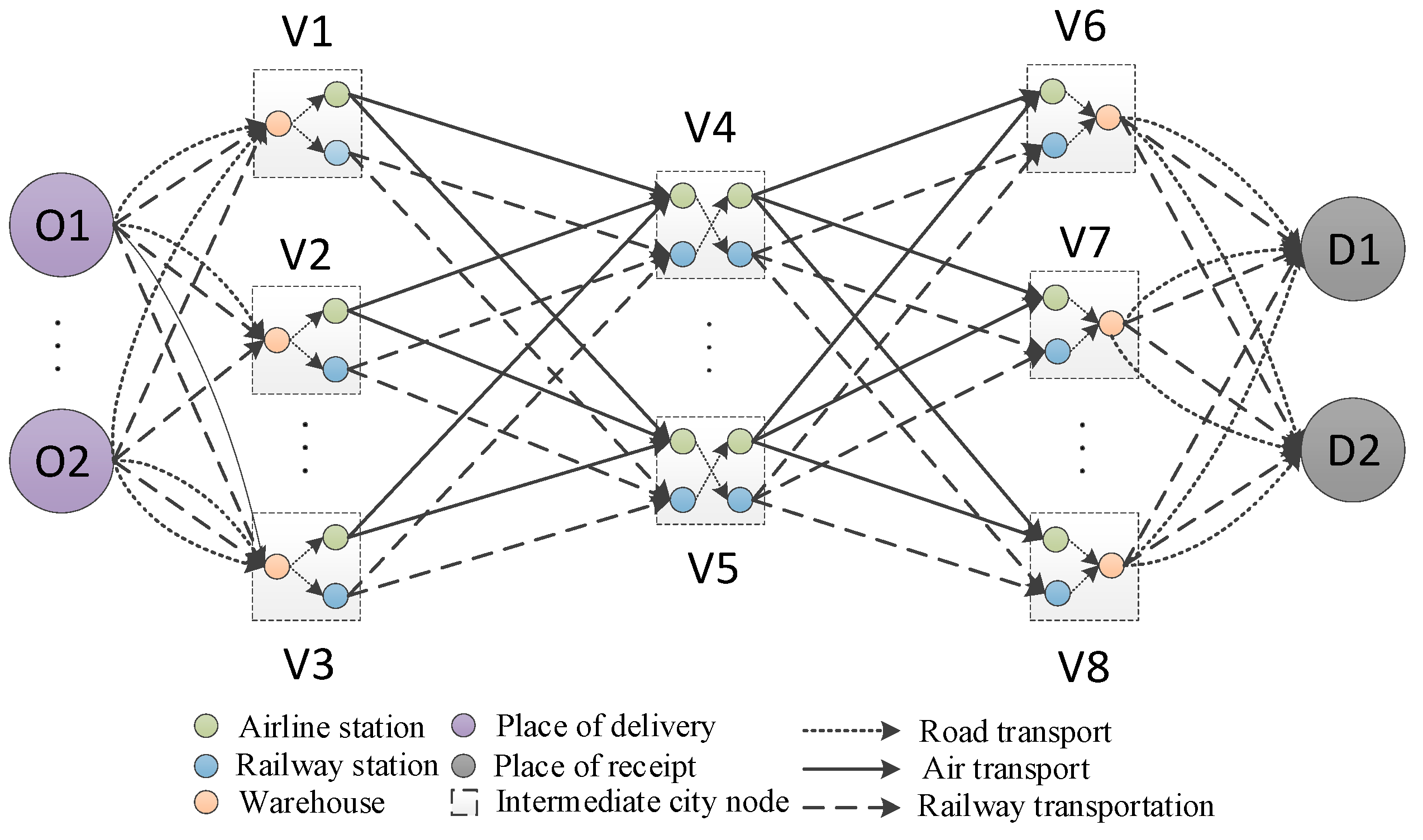
In the actual freight multimodal transportation system, facing the needs of different groups of customers, freight transportation enterprises often need to transport a batch of goods from multiple starting points to multiple destinations. However, there will inevitably be partial overlap in the transportation paths of customer orders, and adopting separate transportation for overlapping orders will increase transportation costs and carbon emissions, resulting in greater waste of resources and reduced transportation efficiency. Order consolidation transportation will help solve this problem. The complete transportation path from the starting point to the destination by the combination of air and high-speed railway needs to be constructed, as illustrated in Figure 1. According to specific strategies, customer orders are consolidated and transported together in suitable segments. Within the shipping and receiving areas, high-speed railways are used. Between the hub nodes, air transport and high-speed railways are selected, both of which have fixed schedule constraints. Waiting for scheduled departures incurs storage costs. The transportation time, cost, and carbon emissions for each mode of transportation between nodes are different. The trans-shipment involves certain trans-shipment costs, time, and carbon emissions. Air and high-speed railways may have some uncertain delay times due to bad weather or breakdowns. When orders arrive beyond the customer’s required time window, a time penalty cost is incurred. The objective is to obtain the optimal combination of transportation modes and routes under different punctuality rates, and then minimize the total transportation cost, transportation time, and carbon emissions for all orders.
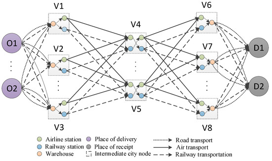
Figure 1.
Schematic diagram of the multimodal transportation network.
Considering the actual situation of multimodal transport and the convenience of mathematical modeling and solving, the following model assumptions are made:
- For the same order, goods should not be split and should only use one mode of transportation between any two nodes.
- Goods trans-shipment should only occur at nodes, and each node should only have one trans-shipment.
- Goods should only select one transportation route and one mode of transportation between two nodes.
- The in-transit transportation speed of each mode of transportation is constant and known.
- After completing trans-shipment at the current node, goods are transported to the next node by the next available schedule of the selected transportation mode.
- In this paper, only flight and high-speed railway time delays are considered, excluding road time delays.
- In-transit and trans-shipment delay times are random variables following a log-normal distribution.
2.2. Order Consolidation Strategy
Assuming a multimodal transport enterprise has several freight orders that need to be transported within a planning period, the initial step is to develop an initial transportation plan for each order. Each initial transportation plan must meet the basic needs of the customer (hereafter, the transportation plans are collectively referred to as tasks in this section). Following a set of rules, one primary task is selected from the N tasks, and the remaining N-1 tasks are referred to as sub-tasks. According to the order consolidation strategy, it is then determined sequentially whether each of the N-1 sub-operations meets the consolidation criteria. If the criteria are met, the task is consolidated, ultimately generating a consolidated transportation plan.
2.2.1. Primary Task Selection Strategy
To enhance the efficiency of order consolidation, the primary task should have characteristics such as large freight volume, long transportation routes, and multiple transportation nodes. Here, the percentage of the traffic volume, line length, and transportation node number of the task in the value of total tasks are defined as , respectively.
Then, the evaluation factor of the task is defined as , where are the weights of each evaluation factor, and .
The following flexible selection strategy is used for choosing the main task: firstly, the variable evaluation factor of each transportation task is calculated and arranged in descending order; then, a fixed constant, , is chosen, randomly generating a lower bound, ; each task is checked one by one starting from the first task, and the coefficient is generated randomly; if , then the task is the main transportation task.
2.2.2. Order Consolidation Conditions
- Time Coordination Constraint: After order consolidation, the transportation plan must satisfy the time coordination constraint, which means the sub-task must arrive at the consolidation point and complete the trans-shipment before the primary task departs from that point.
- Capacity Constraint: After order consolidation, the transportation plan must satisfy the capacity constraint. The consolidation may cause cargo to concentrate in certain advantageous routes, potentially leading to capacity issues.
- Objective Function Optimization: After order consolidation, the value of the objective function must be better than before consolidation.
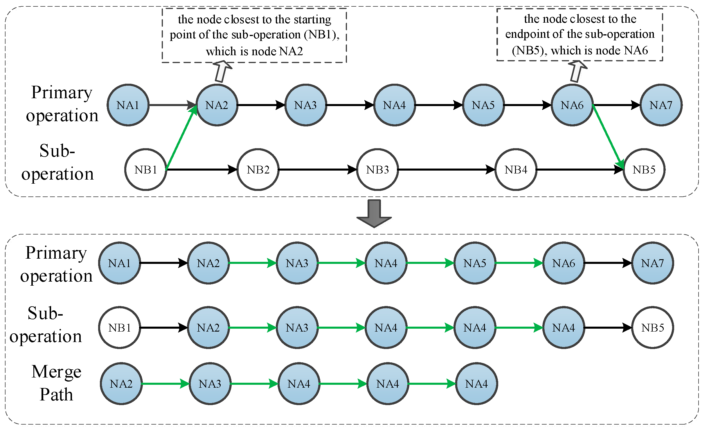
The specific order consolidation strategy is depicted in Figure 2. Consider a primary task, NA1-NA2-NA3-NA4-NA5-NA6-NA7, and a sub-task, NB1-NB2-NB3-NB4-NB5. Initially, all nodes on the primary task route are examined, and the Floyd algorithm is employed to identify the node closest to the starting point of the sub-task (NB1), which corresponds to node NA2. The time coordination constraint is then verified for this node; if satisfied, it is designated as the consolidation point; otherwise, the search continues. Subsequently, all nodes on the primary task route after node NA2 are explored to find the node closest to the endpoint of the sub-task (NB5), identified as node NA6. Consequently, the sub-task route transitions from NB1 to NA2 (via shortest path), proceeds along the primary task route from NA2 to NA6, and finally extends from NA6 to NB5. Following this, verification of capacity constraints takes place; if met, an assessment of whether or not objective function value optimization has been achieved for consolidated transportation plans follows. If not optimized, these steps are repeated until all nodes on the primary task route have been traversed.
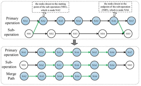
Figure 2.
Order consolidation strategy.
2.2.3. Order Consolidation Scenarios
It is assumed that the order information is known in advance for a given planning period in this study. If the origin of the main order and the sub-order are the same, the multimodal transport operator can negotiate with the shipper to adjust the dispatch time, provided it does not exceed a four-hour window, without affecting the delivery time of the sub-order. This adjustment allows for the consolidation of orders, thereby improving transportation efficiency. Based on the above order consolidation strategy, the following scenarios 1~4 may arise during the order consolidation process:
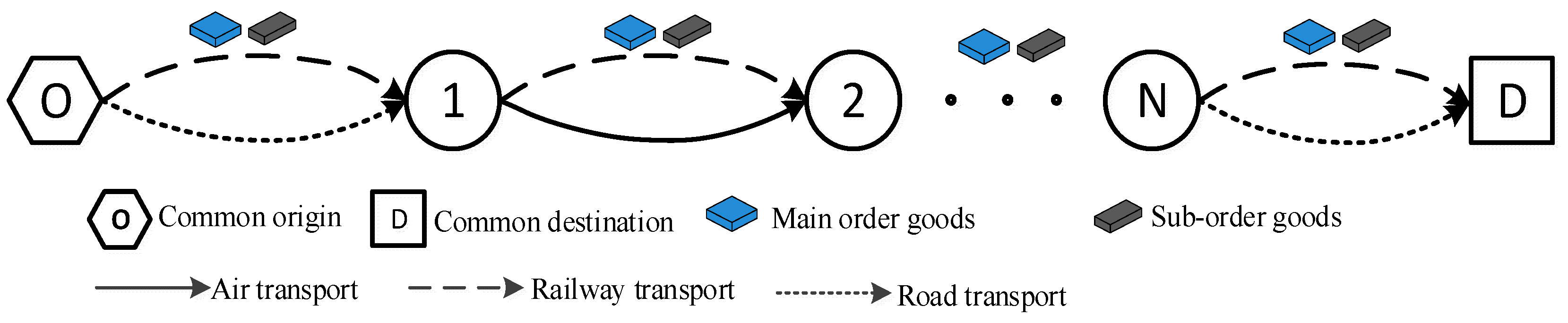
- Scenario 1: Sub-orders and master orders have the same origin and destination. In this scenario, the sub-order is directly combined with the main order for transportation, and the sub-order has the same transportation path and transportation mode as the main order. The specific combined transportation method is shown in Figure 3.
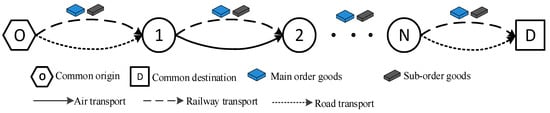 Figure 3. Scenario 1 with the same origin and destination of main orders and sub-orders.
- Scenario 2: Sub-orders and main orders have the same origin but different destinations. In this scenario, the sub-order and the main order are first combined and transported from the origin O to the nearest city node I of the destination of the sub-order, and then they are transported separately from that node to their destinations. The specific combined transportation method is shown in Figure 4.

Figure 4.
Scenario 2 with the same origin and different destinations of main orders and sub-orders.
Figure 4.
Scenario 2 with the same origin and different destinations of main orders and sub-orders.
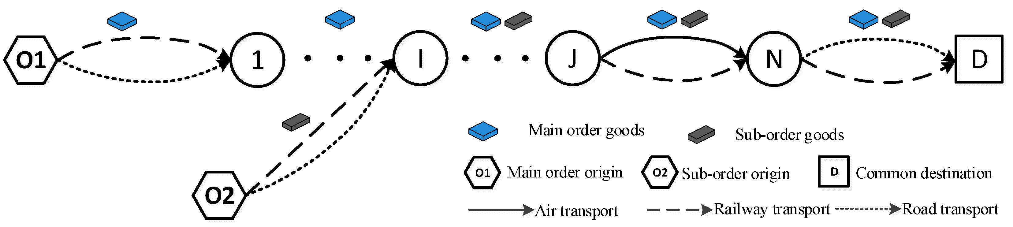
- Scenario 3: Orders have different origins but the sub-order and the main order have the same destination. In this scenario, the sub-order is first transported from its origin to the consolidation city node I on the transportation route of the main order. This node should be the closest city node to the origin of the sub-order that satisfies the time coordination constraint. From this node, the sub-order is consolidated with the main order and they are transported together to the common destination D. The specific consolidation method is illustrated in Figure 5.
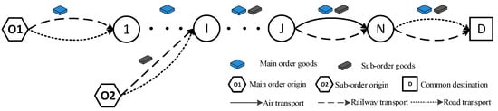
Figure 5.
Scenario 3 with different origins and the same destination of main orders and sub-orders.
Figure 5.
Scenario 3 with different origins and the same destination of main orders and sub-orders.
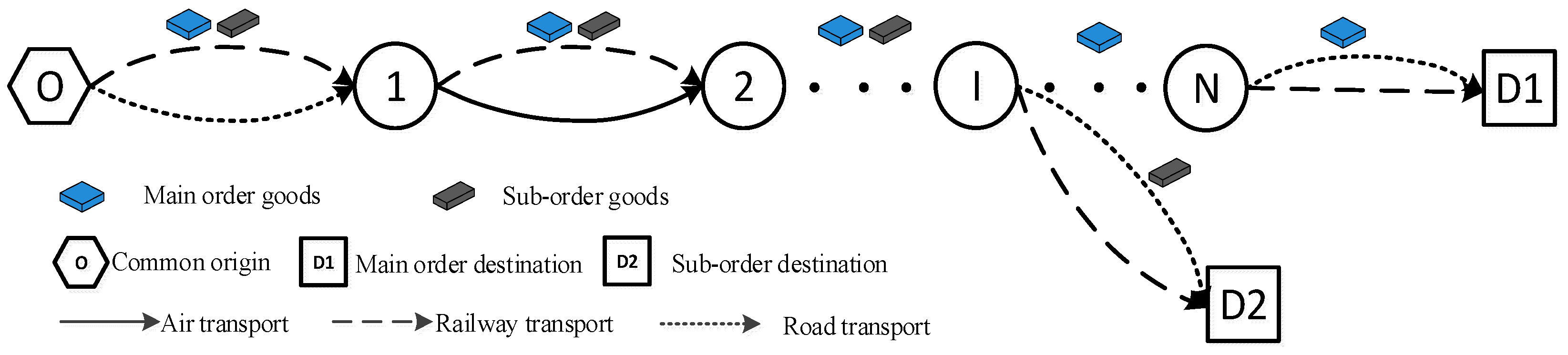
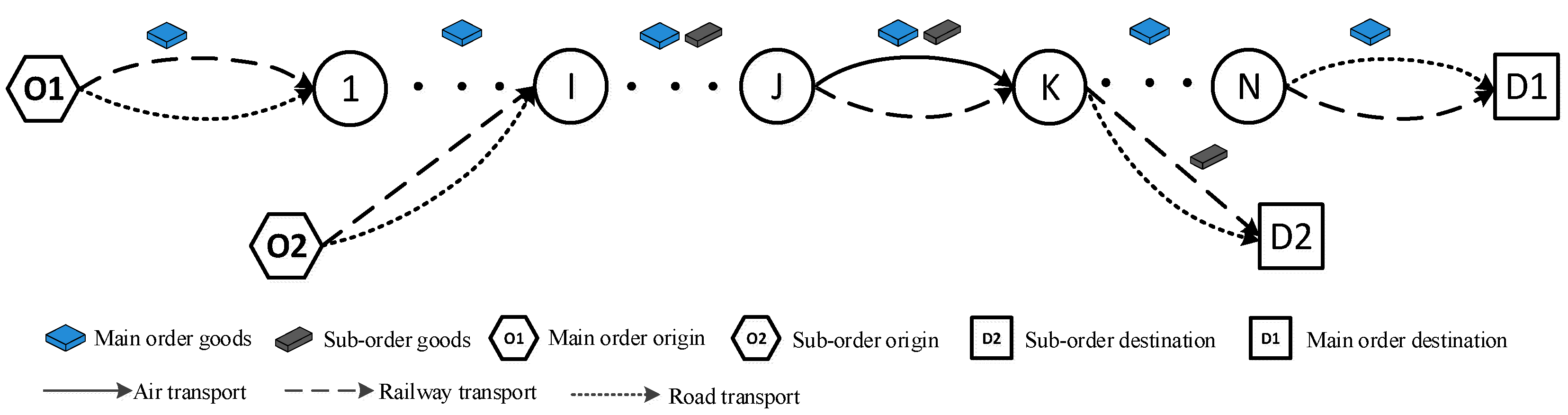
- Scenario 4: The sub-order and main order have different origins and destinations. In this scenario, the sub-order is first transported from its origin, O1, to the consolidation city node I on the main order’s transportation route (this consolidation node should be the closest city node to the origin of the sub-order that satisfies the time coordination constraint). Then, the sub-order is consolidated with the main order and they are transported together to the separation point, K (the separation city node should be the closest city node to the destination of the sub-order). From this node, the sub-order is transported separately to its final destination. The specific consolidation method is illustrated in Figure 6.
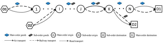 Figure 6. Scenario 4 with different origins and destinations of main orders and sub-orders.
2.3. Model Construction
2.3.1. Symbol Description
The multimodal transport network is abstracted as a graph, , as shown in Figure 1, where is the set of nodes in the network; is the set of transportation modes; and is the set of transportation arcs between two nodes. Each transportation arc includes four types of weights: transportation cost, transportation time, carbon emissions, and transportation distance. Considering order consolidation under uncertain conditions and customer demand differences, the symbols used in the multimodal transport scheme optimization model and their definitions are shown in Table 1.

Table 1.
Symbol descriptions.
2.3.2. Objective Functions
The model constructed in this study aims to minimize transportation cost, transportation time, and carbon emissions while meeting transportation demands. Therefore, the total objective function is established, including transportation cost, total transportation time, and carbon emissions, which will be described in detail separately below.
- 1.
- Transportation cost
- 2.
- Transportation time
- 3.
- Carbon emissions
2.3.3. Constraints
To facilitate the solution of the model and to consider the impact of order consolidation on the model, the following constraints are established.
where Equation (18) indicates that no more than one mode of transport can be used between any two nodes. Equation (19) states that trans-shipment can occur at most once at any node. Equation (20) ensures transportation continuity. Equation (21) represents the balance of freight flow at nodes. Equation (22) specifies the normal transportation time between two nodes. Equation (23) indicates that the required freight volume at any node should be less than the transportation capacity of the mode . Equation (24) represents the total time for order to travel from the origin to a node using the transportation mode . Equation (25) represents the total time for order to travel from the origin to a node and complete the trans-shipment from mode to mode . Equation (26) indicates the total days order spends to reach node using a transportation mode . Equation (27) specifies whether order chooses the schedule of a transportation mode from node to node . Equation (28) represents the time that order waits at node for transport mode to depart, and is 0 when no trans-shipment occurs or trans-shipment is by road. Equation (29) states that the probability of delivering goods within the specified time should be no less than α. Equation (30) indicates no trans-shipment occurs at the origin and destination. Equation (31) represents the 0–1 binary variables. Equations (32) and (33) specify that the total freight volume between two nodes should meet the lower and upper limits of the selected billing level. Equation (34) indicates that for any consolidated order set, the sub-order should arrive at the consolidation node and complete trans-shipment before the main order departs from the consolidation node. Equation (35) states that the objective function value after order consolidation should be less than the objective function value before consolidation. In Equation (36), represents the unit carbon emissions of the transportation mode on the segment ; represents the initial unit carbon emissions of the transportation mode ; represents the number of order consolidations on the segment ; represents the in-transit carbon emissions discount factor, with , , and the discount factor decreases with an increasing number of consolidations. It should be noted that trans-shipment carbon emissions were ignored in the order consolidation and fixed schedules were used, which will have some limitations in the actual transportation. Dynamic scheduling should be considered in future research.
2.3.4. Deterministic Transformation of the Model Based on Fuzzy Credibility
Considering that the model constructed in this paper includes fuzzy freight volume parameters, the model is converted to a deterministic form using chance-constrained programming methods [30]. The objective value is the optimal value of the objective function under the condition that the confidence level is greater than . Therefore, the optimization model with fuzzy parameters can be expressed in the form of Equation (37).
where is the decision variable; is the vector of fuzzy parameters; Pos{} denotes the probability of the event inside the brackets; is the objective function with fuzzy parameters; represents the constraints with fuzzy parameters; is the confidence level of the objective function; is the confidence level of the constraints.
Therefore, a solution to the problem is feasible only if the probability of the constraints is not less than . If the objective function includes fuzzy parameters, multiple possibilities satisfy the condition . Hence, for the minimization problem, the value of the objective function in the optimization model can be expressed in the form of Equation (38).
Since the objective function value and constraints of the constructed model include fuzzy freight volume parameters, the above fuzzy chance-constrained programming method can be used to transform the multimodal transport planning model into the following form:
Objective function:
Constraints:
where Equation (40) represents the minimum value achievable under the confidence level , and Equation (41) indicates that the probability of the freight volume between city nodes and node exceeding their capacity limit is not less than the confidence level .
According to Sun et al. [31], when a deterministic number and a trapezoidal fuzzy number are given, using fuzzy credibility, they have the following relationship:
Based on Equation (42), the objective function and constraints containing fuzzy numbers can be clarified. It is known that when the confidence level of the customer’s fuzzy freight volume is , and , the parameter in the objective function and constraints can be converted to
When the confidence level of the customer’s fuzzy freight volume is , and , the parameter in the objective function and constraints can be converted to
3. Solution Algorithm Design
In this section, we design a basic genetic algorithm (GA), develop an improved genetic algorithm based on stochastic simulation techniques to address the characteristics of the model with random delay times, and then propose an improved genetic algorithm based on the task riding method for order consolidation.
3.1. Basic Genetic Algorithm
- 1.
- Coding and Decoding
This paper adopts a real-number coding method. A single order consists of two chromosome segments: the first segment is the transportation node coding, and the second segment is the transportation mode coding. The transportation modes are represented by 1, 2, and 3, corresponding to air, rail, and road transportation modes, respectively. Figure 7 illustrates the encoding and decoding process. Suppose there are orders in total. The individual transportation plans for each order are combined to generate a multi-order transportation plan individually, as shown in Figure 8.
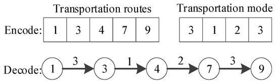
Figure 7.
Encoding and decoding.
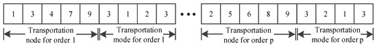
Figure 8.
Composition of multiple chromosomes.
- 2.
- Population Initialization
The population initialization method is designed based on the characteristics of the multimodal transport network. The specific steps are as follows:
- Step 1: Generate the adjacency matrix and the matrix of transportation modes existing between any two nodes based on the multimodal transport network. For the adjacency matrix, nodes are connected if there is a transportation mode between two nodes.
- Step 2: Generate legitimate transportation paths based on the topological sorting rules combined with the adjacency matrix . The node numbers in the path are used as the coding for chromosome segment one. Then, randomly select any transportation mode between nodes from the matrix to generate chromosome segment two, thus obtaining the single-order transportation plan chromosome. This process is repeated until the desired number of single-order transport plan chromosomes is generated, and they are combined to obtain the individuals of the initial population.
- Step 3: Stop if the population size meets the requirement; otherwise, return to step 2.
- 3.
- Selection Operation
To avoid irrationality in the selection of populations, the selection method was improved and is as follows: first, sort the individuals in the population in descending order of fitness values; then, duplicate the top 25% of individuals to form 50% of the new population; directly place the individuals ranged from 25% to 50% into the new population; calculate the similarity of all individuals in the population to the current optimal individual; sort the individuals in descending order of similarity; and select the individuals with the highest similarity to complete the new population. The similarity calculation method is shown in Equation (45).
In the formula, D represents the similarity, n represents the number of objective functions, represents the value of the objective function for the individual , and represents the value of the current best individual’s objective function.
- 4.
- Crossover Operation
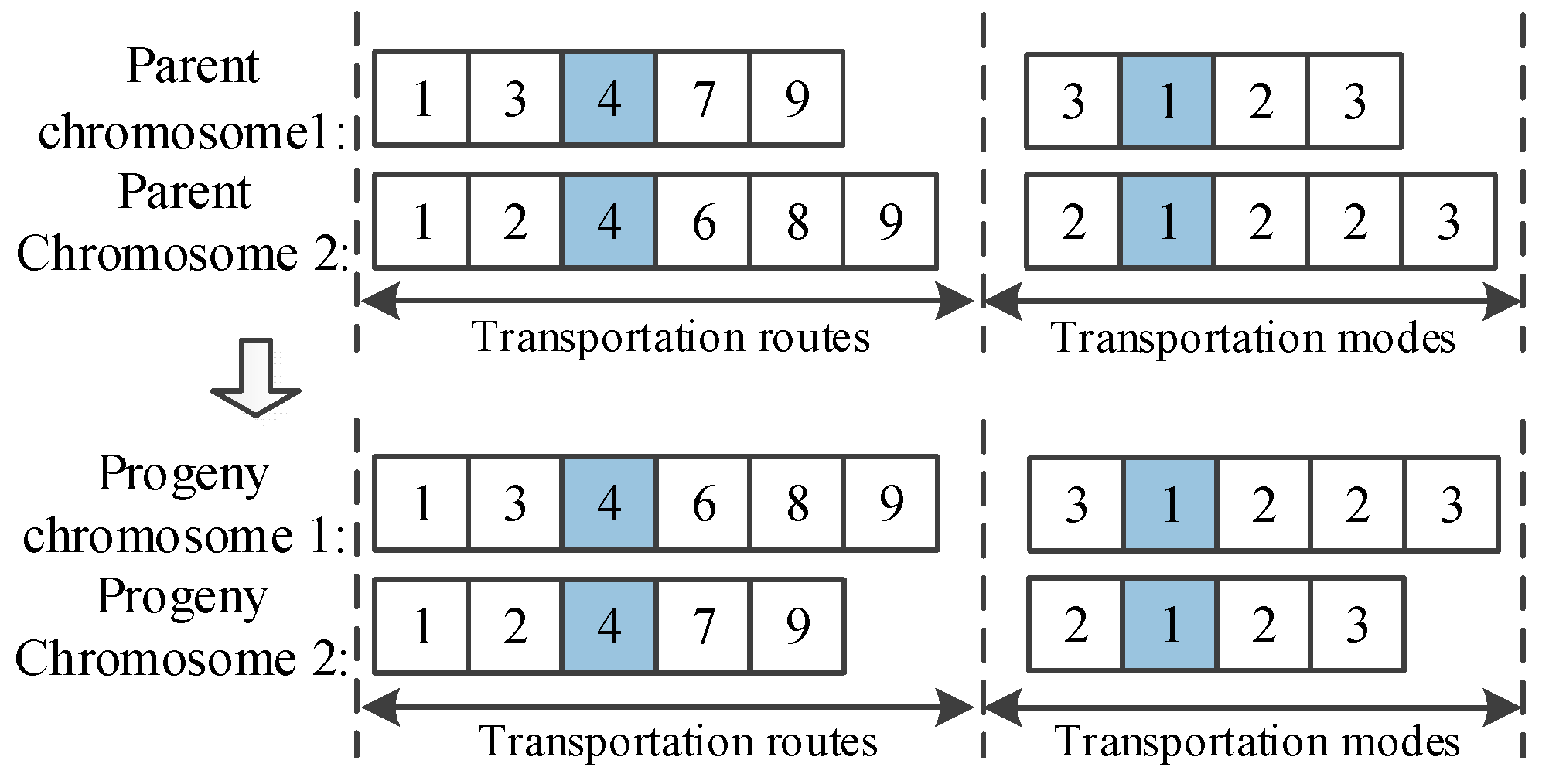
There are two cases of chromosome crossover selection. The first case is that there are the same nodes between the two parent chromosomes except the origin and the endpoint. The second case is that there is no node in common between the two parent chromosomes. In order to prevent errors in the starting and ending point information, an improved single-point crossover method is designed in this paper.
For the first case, a common node from the parent chromosomes is chosen as the crossover point. If there are multiple common nodes, one is randomly selected, and then the gene segments after the crossover point are exchanged to produce two new chromosomes. These two chromosomes are feasible, which is illustrated in Figure 9.
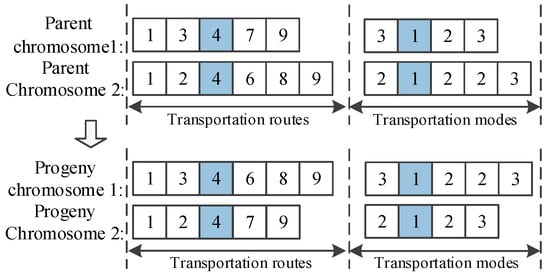
Figure 9.
Crossover at the same node for the first case.
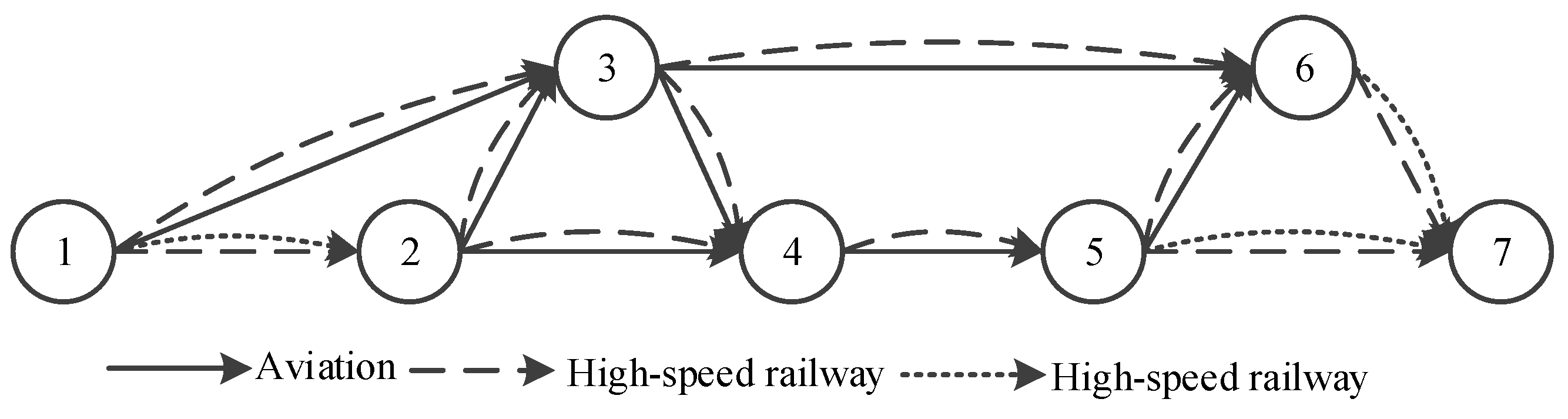
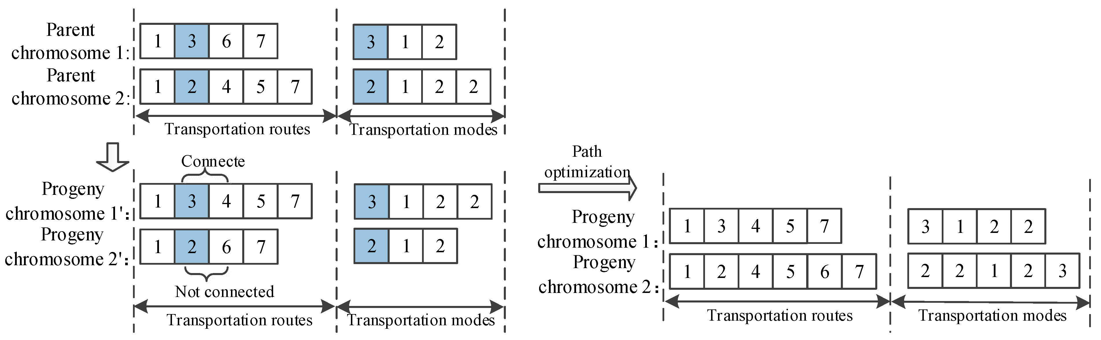
Since real-world networks are often incomplete, illegal individuals may be generated during the crossover process for the second case. As shown in Figure 10, node 1 is the origin, and node 7 is the destination. Two legal paths, 1-3-6-7 and 1-2-4-5-7, are selected as parent chromosomes. From Figure 11, a gene position {3,2} is randomly selected for the crossover operation. However, because there is no transportation arc connecting nodes 2 and 6, the resulting sub-path 2 is an illegal path. Therefore, the Floyd algorithm must be used to find a valid path from node 2 to node 6, making the offspring chromosome 2 a valid transportation plan.

Figure 10.
Schematic diagram of multimodal transport network.
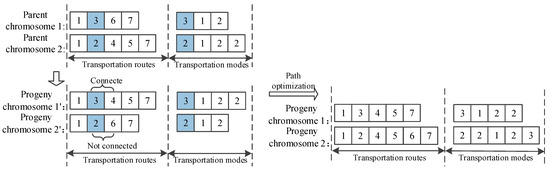
Figure 11.
Crossover at the same gene position for the second case.
- 5.
- Mutation Operation
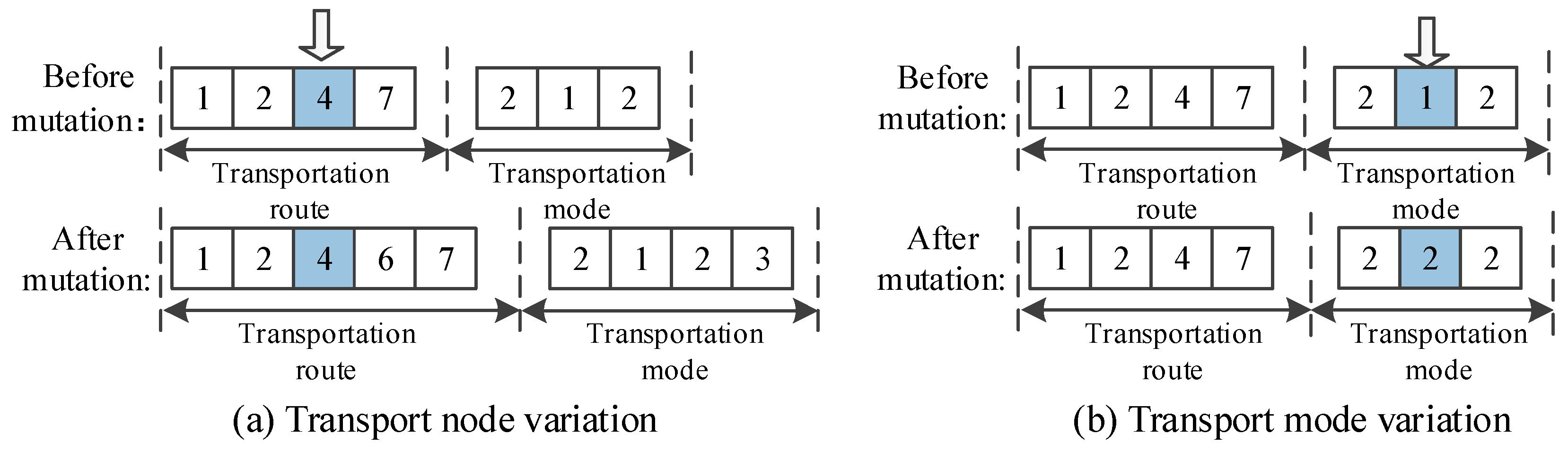
Before mutation, the individuals in the population are first decomposed into clusters in order, and then the mutation operation is performed within each order cluster. Two cases need to be equally considered in the mutation process: the first case is that the mutation point is in chromosome segment one, and the second case is that the mutation point is in chromosome segment two.
For the first case, as shown in Figure 12a, a random node (e.g., node 4) is selected. The Floyd algorithm is used to find a valid path from node 4 to node 7. Chromosome segment two then randomly fills in valid genes according to the mutated genes in chromosome segment one to complete the mutation.
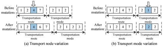
Figure 12.
Chromosome mutation.
For the second case, as shown in Figure 12b, a mutation position is randomly selected from chromosome segment two. It is then determined whether there are other transportation modes available between the corresponding nodes. If there are, a new transportation mode is randomly selected to replace the original mode; otherwise, no mutation occurs.
3.2. Improved Genetic Algorithm Based on Stochastic Simulation Technique
- 1.
- Objective Function Value Calculation
Considering the uncertainty of delay times represented by random variables, the objective function value of the transportation scheme cannot be accurately calculated. A stochastic simulation technique is introduced in the present study. By performing multiple simulations, a sufficient number of samples for the objective function values are obtained and the final objective function value of the scheme is estimated through the average value of the sample. The stochastic simulation algorithm is shown in Table 2.
Table 2.
Stochastic simulation algorithm.
- 2.
- Fitness Values and Constraint Handling
The model built in this paper has a total of three objective function values, and all of them have the minimum value as the optimization objective; therefore, the inverse of the objective function is used as the fitness function, as shown in Equation (46).
To achieve the purpose of deleting illegal solutions, this paper assigns the objective function values to the individuals that do not satisfy the constraints. In this case, the on-time rate of the individual is calculated as follows:
- Step 1: Input the individual, assuming there are p orders to be decided.
- Step 2: Uniformly generate N samples based on the delay time probability distribution function.
- Step 3: Calculate the transportation time of each order in the individual under each sample.
- Step 4: Count the number of samples where the transportation time of each order is within the delivery time window.
- Step 5: Calculate the punctuality rate of each order in the individual, .
- Step 6: Calculate the individual’s punctuality rate . If the punctuality rate constraint is not met, set the fitness to zero; otherwise, .
3.3. Improved Genetic Algorithm Based on Task-Riding Method
Based on the above algorithm, the transportation plans (hereinafter referred to as “tasks”) that meet the basic conditions for each order are obtained, and then an initial main task is selected from these tasks. The remaining tasks become sub-tasks. Then, one sub-task is selected to determine if it meets the order consolidation conditions. If it does, the sub-task is included in the order consolidation set; otherwise, the remaining sub-tasks are sequentially selected to determine if they can be consolidated. This process continues until all sub-tasks have been examined, resulting in the first-order consolidation set. A new main task is then selected from the remaining non-consolidated tasks, and the above steps are repeated to generate the second-order consolidation set. This iterative process continues until the entire order consolidation transportation plan is generated. The specific flow is shown in Table 3.
Table 3.
Task-riding algorithm.
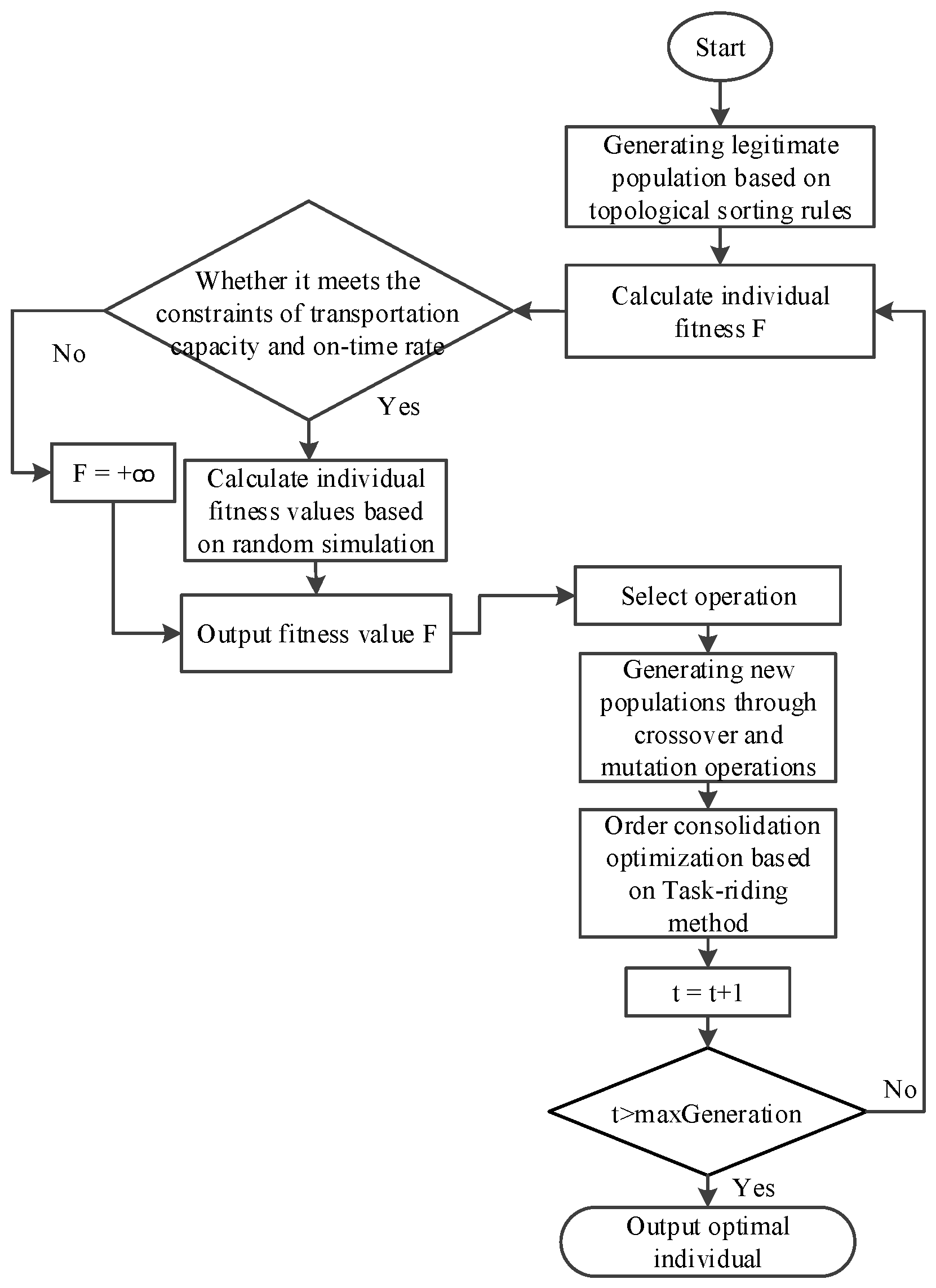
3.4. Algorithm Flowchart
The overall process of the improved genetic algorithm combined with the task-riding method is shown in Figure 13.
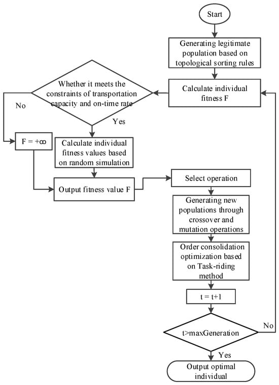
Figure 13.
Flowchart of improved genetic algorithm for solving the order consolidation problem.
4. Case Analysis
4.1. Case Description and Parameter Setting
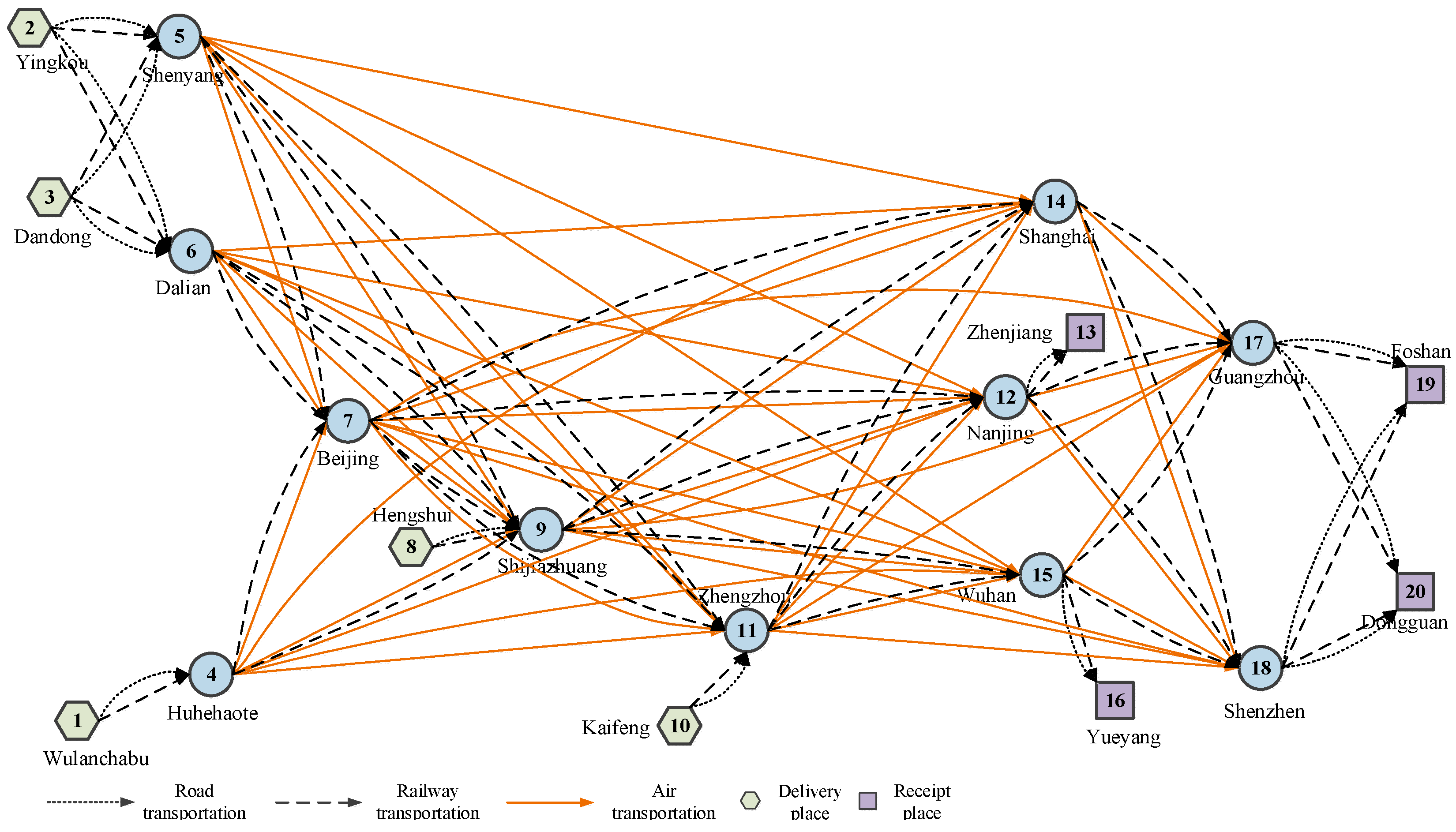
Consider that in reality, within a planning period, orders received by a multimodal transport company may be dispersed and have different starting and receiving points. To better align with actual conditions and explore the impact of multiple origins and destinations on the benefits of order consolidation, five shipping points and four receiving points are set, with some of these points located in the middle of the network. The specific structure of the multimodal transport network is shown in Figure 14. The order details and related parameters for transportation are shown in Table 4, Table 5, Table 6, Table 7, Table 8, Table 9, Table 10 and Table 11. Table 4 provides the transportation distance data between node pairs. Table 5 shows the capacity constraints data of different modes of transportation in each transport arc, which determines the final transportation times and order combination mode. Table 6 is the baseline order information, including the origin–destination, dispatch time, delivery deadline, and fuzzy freight weight. Table 7 gives the four order consolidation scenarios as introduced in Section 2.2.3, but the information on dispatch time, delivery deadline, and fuzzy freight weight are the same as in Table 6. Table 8, Table 9, Table 10 and Table 11 give the parameters of the time, speed, cost, and carbon emissions in each transport mode.
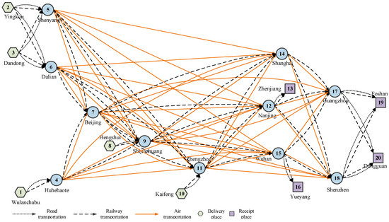
Figure 14.
Multimodal transport network diagram.
Table 4.
Transportation distance data between node pairs.
Table 5.
Capacity constraints of different modes of transportation in each transport arc.
Table 6.
Baseline Order details.
Table 7.
Origin and destination of orders in each scenario.
Table 8.
Parameters related to transportation modes.
Table 9.
Schedule of departures.
Table 10.
Parameters related to trans-shipment.
Table 11.
Parameters for trans-shipment and in-transit transportation delays.
4.2. Results Analysis of Scheme Optimization with and without Order Consolidation
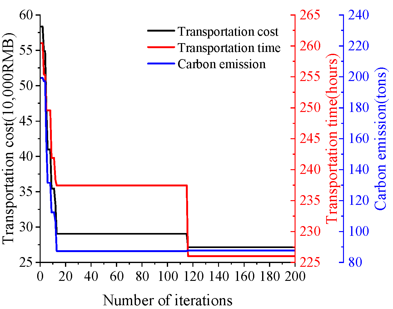
Taking Order Scenario 4 as an example, the solution was obtained using MATLAB R2022a. After repeated pre-testing, the number of random simulations N was set to 1000, the initial population size was 100, the maximum number of genetic iterations was 200, the crossover probability was 0.9, the mutation probability was 0.3, the probability of the opportunity constraint for on-time delivery was 0.6, the fuzzy preference value for demand quantity was 0.6, and the weights of the objective functions were all 1/3. The convergence of each objective function is shown in Figure 15, where convergence was reached at around iteration 118. The optimal transportation scheme for order consolidation is shown in Figure 16.

Figure 15.
Convergence of objective function values.
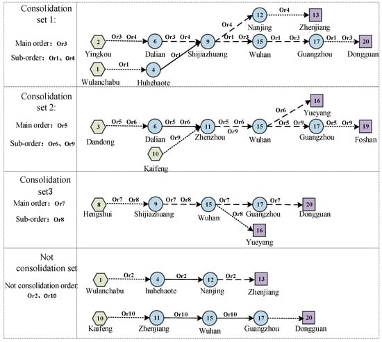
Figure 16.
Combined transportation plan for orders.
To investigate the effect of order consolidation on the optimization results of the transportation scheme, the percentage change in the objective function value before and after order consolidation was defined as shown in Equation (47).
where is the scheme objective function value after consolidation, and is the scheme objective function value before consolidation.
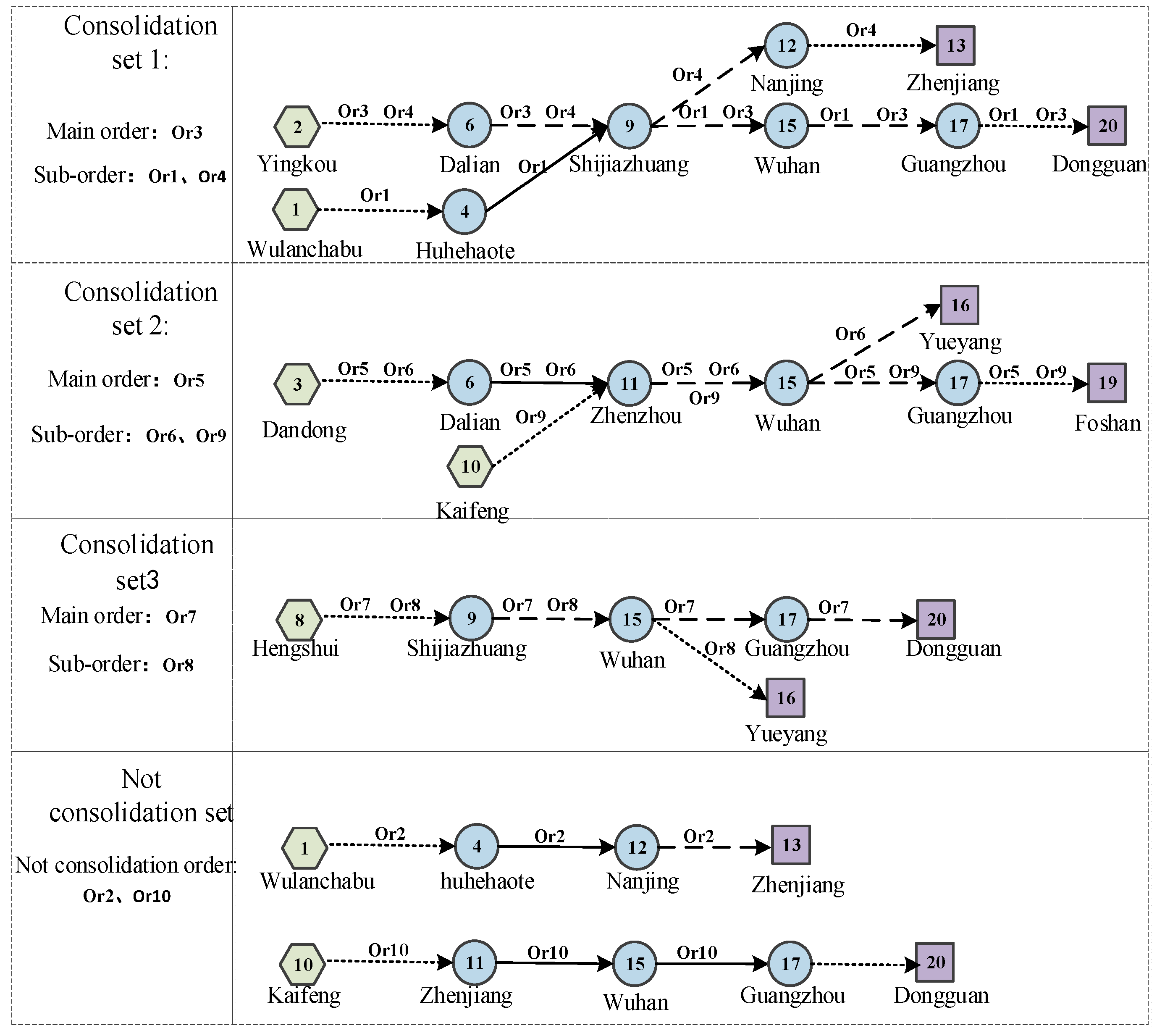
The total transportation cost, time, and carbon emissions of the scheme before and after order consolidation were calculated, as well as the value of each order, respectively. The results are shown in Table 12. It can be seen that after the consolidation, the total cost is 271,577 RMB, which has a decrease of 16.6%; the total carbon emission is 87.8 t, which has a decrease of 24.69%; the total time is 211.04 h, which has an increase of 5.56%. Most of the orders have decreased in transportation cost and carbon emissions and increased in transportation time compared with no consolidation, such as Or1, Or3, Or6, Or7, etc. However, a single order may increase the transportation cost and carbon emissions and reduce transportation time, such as Or10, which indicates that in order to seek the overall optimization of the scheme, the benefits of some orders may be lost with order consolidation. The above results verify the advantages of the designed order consolidation strategy and algorithm in reducing transportation costs and carbon emissions. This also suggests that intermodal operators need to consider the global situation and uniformly transport and plan multiple orders with different origin and destination and time window constraints to seek overall optimization.
Table 12.
Comparative analysis of results with and without order consolidation.
4.3. Impact of Customer Preferences on Order Consolidation
To explore the impact of customer preferences on order consolidation, the parameters for different customer types were calculated, which include four customer types, i.e., price-sensitive type 1, time-sensitive type 2, timeand price-sensitive type 3, and time- and carbon emission-sensitive type 4. The results are shown in Figure 17, and the values of the customer categories and the corresponding weights are shown in Table 13.

Figure 17.
Results of the parameters for different customer types.
Table 13.
Objective function value weights for different types of customers.
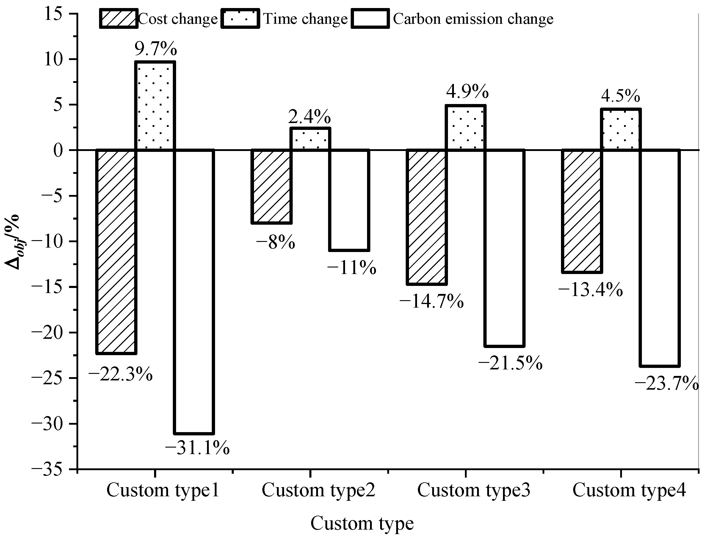
From Figure 17, for all four customer types, both transportation cost and carbon emissions decrease, while transportation time increases compared with no order consolidation. For time-sensitive customers, a 2.4% increase in transportation time, an 11% decrease in transportation cost, and an 8% decrease in carbon emissions occur after order consolidation compared with no consolidation, which is the smallest compared with the other customer types. This is because order consolidation may increase the transportation time for each order, and when customers have high expectations for transportation time, the orders of consolidated transportation will decrease. But for cost-sensitive customers, a 9.7% increase in transportation time, a 22.3% decrease in transportation cost, and a 31.1% decrease in carbon emissions occur after order consolidation compared with no consolidation, which is the largest compared with the other customer types. The reason is that order consolidation can directly reduce transportation costs, and when customers have a strong preference for reducing costs, they are more likely to choose plans with more consolidated orders. The changes in the values of the objective functions for timeand price-sensitive customers and timeand carbon emission-sensitive customers are intermediate. This indicates that order consolidation has positive effects for all customer types, and the effects become more significant as the preferences increase of customers for cost and carbon emissions.
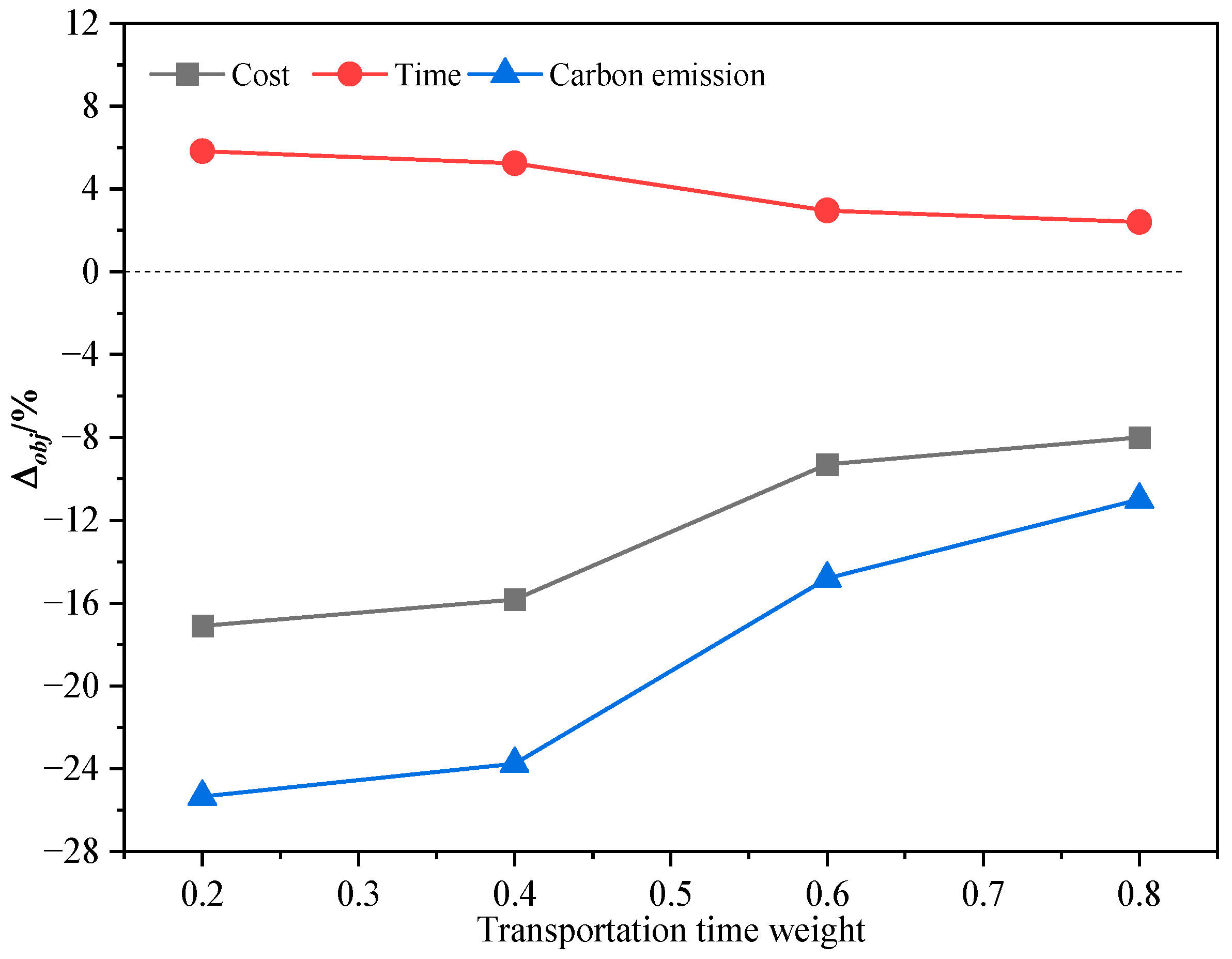
To further investigate the influence of the transportation time preference degree on order consolidation, four scenarios with different weights of 0.2, 0.4, 0.6, and 0.8 for the time objective function are set sequentially, and the other objective function values are the average value of the remaining weights that can be assigned. The values of each objective function with the increase in the transportation time weight are shown in Figure 18. It can be seen that compared with no order consolidation, with the increase in the transportation time weight, the increase rate of total transportation time and the decrease rate of total transportation cost and carbon emission both decrease. This indicates that when the degree of customers’ preference for transportation time is greater, their expectation of order consolidation is smaller, and order consolidation transportation will be less frequent.
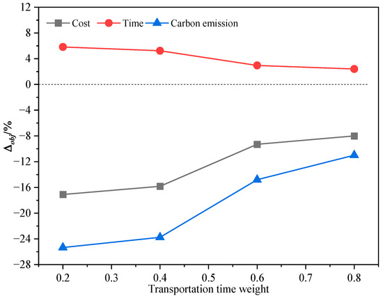
Figure 18.
The variation trend in with increasing transportation time weight.
4.4. Analysis of Order Consolidation Results under Different Scenarios
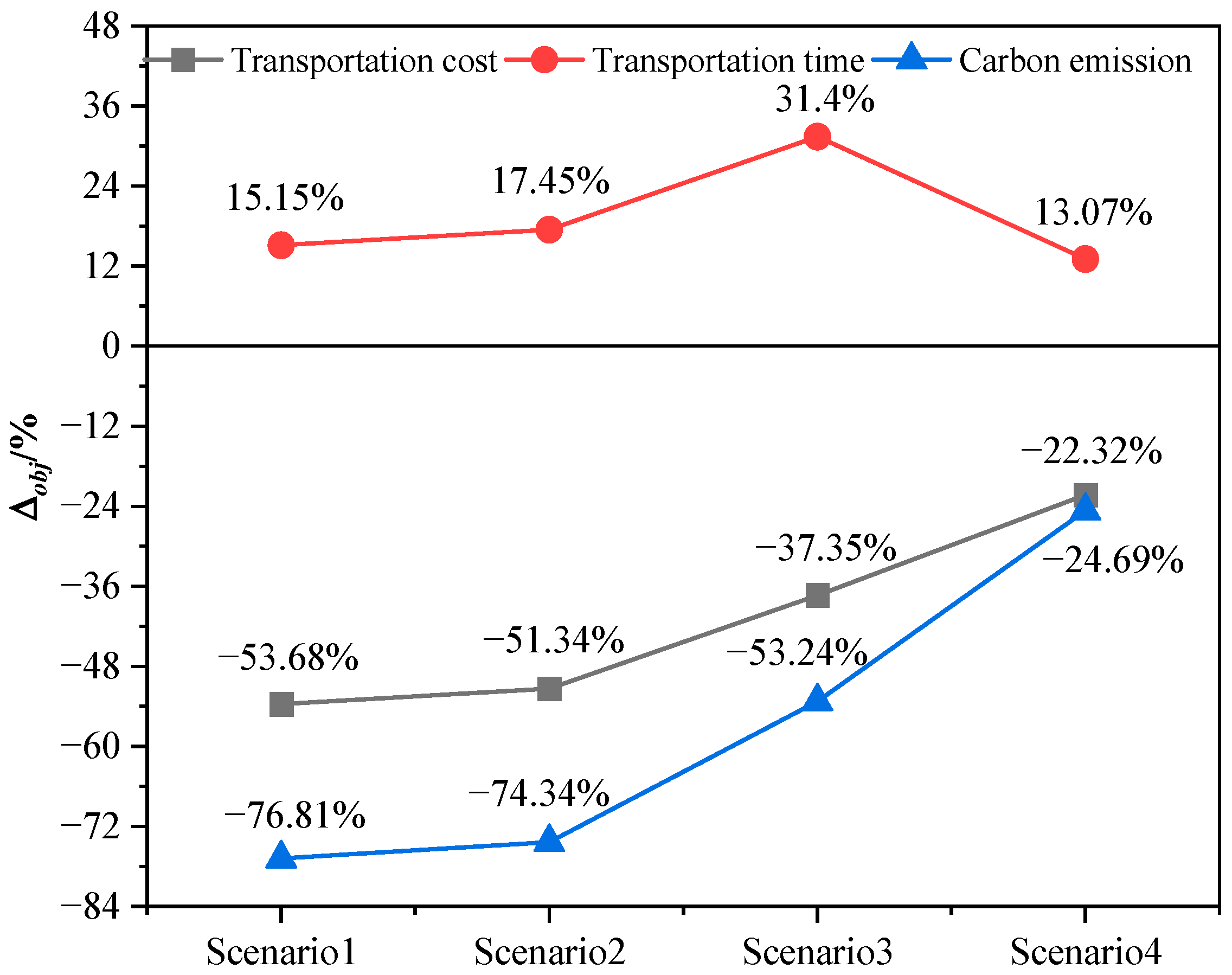
The influences of order consolidation for different transportation scenarios shown in Section 2.2.3 are further analyzed here. Figure 19 shows the results of the percentage change in the objective function values of different scenarios before and after consolidation. It can be seen that the transportation cost and carbon emissions both decrease, but the transportation time increases after consolidation. For the transportation cost and carbon emissions under different scenarios, the most significant reduction was obtained for Scenario 1 with decreases of 53.68% and 76.81%, followed by Scenario 2, Scenario 3, and Scenario 4. For Scenario 1, with the same origin and destination of main orders and sub-orders, the merging transportation of the whole path can be easily completed through the appropriate adjustment of sub-order shipment time. With the gradual increases in origins and destinations for other scenarios, the transportation time will increase due to the search for the separation points, increasing transit time, and the waiting time of the main order for the sub-orders, which eventually leads to the decrease in the reduction in the transportation cost and carbon emissions.

Figure 19.
Benefits of order consolidation in different scenarios.
For transportation time under different scenarios, the value of Scenario 3, with different origins and the same destination of main orders and sub-orders, is the largest, at 31.4%, and the value increases gradually from Scenario 1 to Scenario 3, but the smallest value occurs for Scenario 4. Compared with Scenario 2, with the same origin and different destinations, the transportation time of Scenario 3 shows a 16.25% increase, which indicates that the time consumed waiting for the main order at the merging point is much longer than that consumed for the splitting of sub-orders to transport them from the separating point. Multimodal operators should try to avoid time constraints when formulating a transportation plan for order merging for time-sensitive customers. The percentage change in the transportation time of Scenario 4 is smaller than that of Scenario 1, which may be due to the increased restrictions on order consolidation, resulting in more unconsolidated orders. Therefore, when developing a consolidated transportation plan for orders, multimodal operators should try to avoid orders with different origins, especially those with long distances between origins.
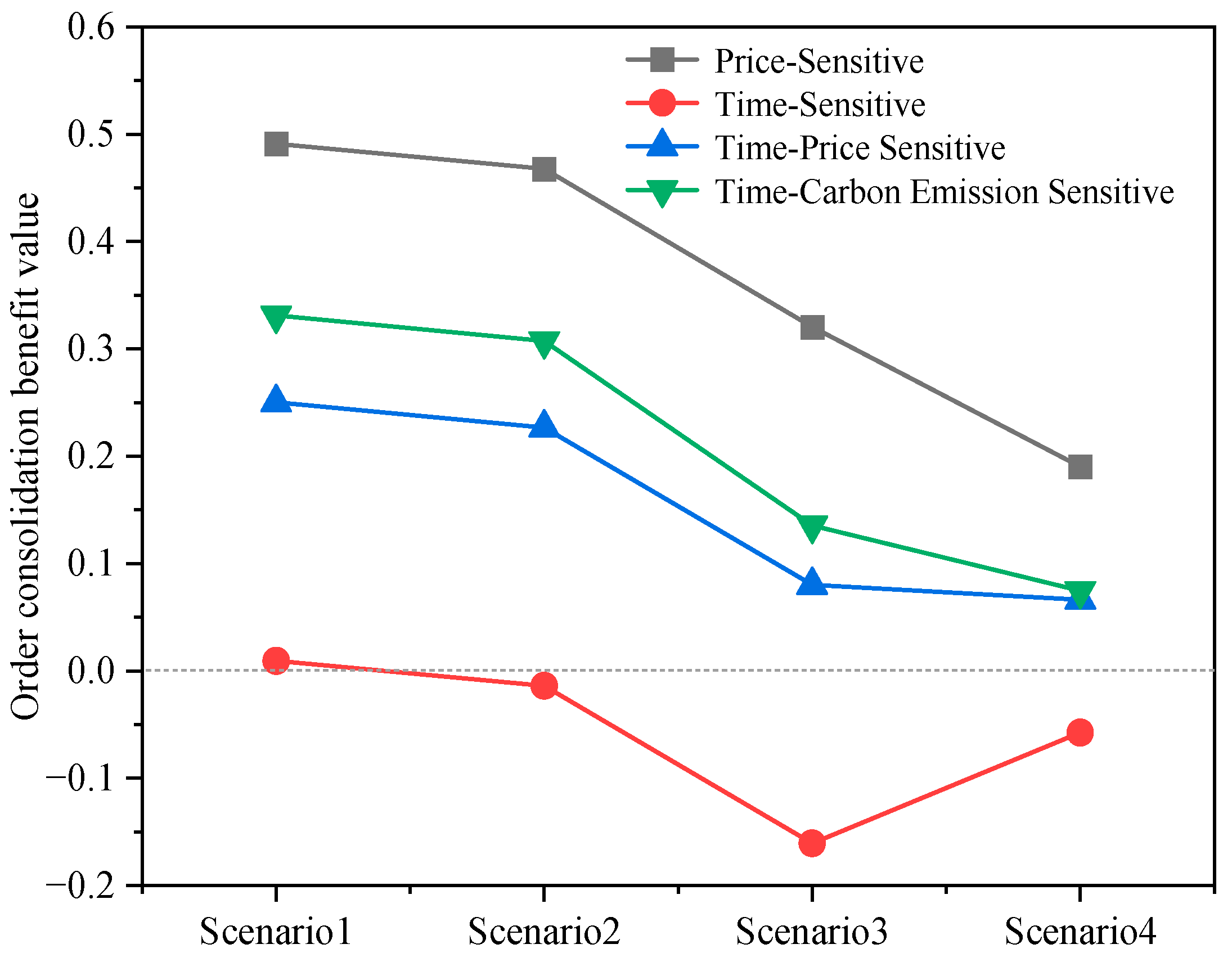
To further explore the preference levels of different customer types for order consolidation in various scenarios, the order consolidation benefit value is defined as shown in Equation (48).
where , , and represent the percentage changes in transportation cost, transportation time, and carbon emissions, respectively, after consolidation, and , , and are the weights of customer preferences for transportation cost, transportation time, and carbon emissions, . And then, substituting the percentage changes in the objective function value in each scenario into Equation (43), the order consolidation benefit values will be obtained for different customer types in various scenarios, as shown in Figure 20. It can be seen that the price-sensitive, time and price-sensitive, and time and carbon emission-sensitive merger benefit values are all greater than 0, which indicates that all three types of customers are willing to engage in order consolidation under each scenario. For time-sensitive customers, only order consolidation under Scenario 1 is meaningful, and the consolidation benefit values under the rest of the scenarios are negative, which indicates that under Scenario 2, Scenario 3, and Scenario 4, time-sensitive customers have negative attitudes towards order consolidation; therefore, when planning transportation scenarios, multimodal operators should fully consider the differentiated needs of the customers and reasonably formulate transportation scenarios for different order scenarios.
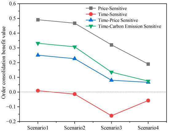
Figure 20.
Order consolidation benefit values for different customer types in each scenario.
5. Conclusions
This paper examines the optimization of multimodal transport schemes, considering order consolidation under uncertainty conditions. Air and high-speed railway multimodal transport is selected, and uncertain delay times, time window constraints, and differentiated customer needs are also considered. The optimization model aims to minimize total transportation cost, time, and carbon emissions while meeting delivery time windows, punctuality rates, and capacity constraints. An improved genetic algorithm combined with a ride-sharing scheduling method is designed. Empirical verification demonstrates both the feasibility of the optimization model and the effectiveness of the solution method.
The results show that with the increase in the number of origin–destination pairs, order consolidation will reduce multimodal transport costs and carbon emissions but increase transportation time, and the advantages of cost and carbon emission reduction will vary with different origin–destination scenarios, which are ranked in the order of single-origin single-destination, single-origin multi-destination, multi-origin single-destination, and multi-origin multi-destination. Taking the fourth scenario as an example, the cost and carbon emissions decrease by 16.6% and 26.69%, respectively, and the time increases by 5.56% compared with no consolidation. This validates the benefits of the proposed order consolidation strategy and algorithm in mitigating transportation costs and carbon emissions, aiming for an overall optimal solution through task consolidation and multi-order planning. In addition, for the sensibility of customer demands, it is found that order consolidation has an advantage for price-sensitive, time and price-sensitive, as well as time and carbon emission-sensitive customers for all order scenarios; however, it is specifically beneficial for time-sensitive customers only in single-origin single-destination scenarios.
In the future, further studies will focus on the dynamic scheduling constraints of air and high-speed rail transportation to improve the model’s potential to solve real-world complex scenarios. Then, we will try to develop an application-type interface for users to provide technical support to multimodal transport operators.
Author Contributions
Conceptualization, P.Z. and Q.S.; methodology, P.Z., C.K. and X.L.; software, X.L. and C.K.; validation, P.Z. and W.C.; formal analysis, P.Z.; investigation, P.Z. and X.L.; resources, Q.S.; data curation, C.K. and X.L.; writing—original draft preparation, C.K. and X.L.; writing—review and editing, P.Z., Q.S. and W.C.; visualization, C.K. and X.L.; supervision, P.Z.; project administration, P.Z.; funding acquisition, P.Z. and Q.S. All authors have read and agreed to the published version of the manuscript.
Funding
This research was funded by the National Natural Science Foundation of China, grant number U2233208, the Opening Fund of the Key Laboratory of Civil Aviation Thermal Disaster Prevention and Emergency, Civil Aviation University of China, grant number RZH2021-KF-02, the Opening Fund of the Key Laboratory of Civil Aviation Emergency Science & Technology (CAAC), Nanjing University of Aeronautics and Astronautics, grant numbers NJ2022022 and NJ2023025.
Institutional Review Board Statement
Not applicable.
Informed Consent Statement
Not applicable.
Data Availability Statement
The original contributions presented in the study are included in the article; further inquiries can be directed to the corresponding author.
Conflicts of Interest
The authors declare no conflict of interest.
References
- Ralf, E.; Jan, P.M.; Johannes, R. Tactical network planning and design in multimodal transportation—A systematic literature review. Res. Transp. Bus. Manag. 2020, 35, 100462. [Google Scholar]
- Delbart, T.; Molenbruch, Y.; Braekers, K.; Caris, A. Uncertainty in intermodal and synchromodal transport: Review and future research directions. Sustainability 2021, 13, 3980. [Google Scholar] [CrossRef]
- Lu, Y.P.; Chen, F.; Zhang, P. Multi-objective Optimization of Multimodal Transportation Route Problem Under Uncertainty. Eng. Let. 2022, 30, 1640–1646. [Google Scholar]
- Xu, Z.; Jin, F.Y.; Yuan, X.M.; Zhang, H.Y. Low-Carbon Multimodal Transportation Path Optimization under Dual Uncertainty of Demand and Time. Sustainability 2021, 13, 8180. [Google Scholar] [CrossRef]
- Lu, Y.; Lang, M.X.; Sun, Y.; Li, S.Q. A fuzzy intercontinental road-rail multimodal routing model with time and train capacity uncertainty and fuzzy programming approaches. IEEE Access 2020, 8, 27532–27548. [Google Scholar] [CrossRef]
- Qi, Q.Y.; Kwon, O.K. Exploring the Characteristics of High-Speed Rail and Air Transportation Networks in China A Weighted Network Approach. J. Int. Logist. Trade 2021, 19, 96–114. [Google Scholar] [CrossRef]
- Li, L.; Zhang, Q.W.; Zhang, T.; Zou, Y.B.; Zhao, X. Optimum Route and Transport Mode Selection of Multimodal Transport with Time Window under Uncertain Conditions. Mathematics 2023, 11, 3244. [Google Scholar] [CrossRef]
- Savoji, H.; Mousavi, S.M.; Antucheviciene, J.; Pavlovskis, M. A Robust Possibilistic Bi-Objective Mixed Integer Model for Green Biofuel Supply Chain Design under Uncertain Conditions. Sustainability 2022, 14, 13675. [Google Scholar] [CrossRef]
- Zhou, Q.; Wang, Z.; Chen, J.M.; Tseng, M.L.; Luan, H.M.; Ali, M.H. Modelling green multimodal transport route performance with witness simulation software. J. Clean. Prod. 2020, 248, 119245. [Google Scholar]
- Ziaei, Z.; Jabbarzadeh, A. A multi-objective robust optimization approach for green location-routing planning of multi-modal transportation systems under uncertainty. J. Clean. Prod. 2021, 291, 125293. [Google Scholar] [CrossRef]
- Peng, Y.; Yong, P.C.; Luo, Y.J. The route problem of multimodal transportation with timetable under uncertainty: Multi-objective robust optimization model and heuristic approach. RAIRO-Oper. Res. 2021, 55, S3035–S3050. [Google Scholar] [CrossRef]
- Boyaci, A.C.; Gencer, C. A bi-objective multi-commodity model for multimodal transportation of hazardous materials: A case study of Turkey. J. Fac. Eng. Archit. Gaz. 2021, 36, 13–26. [Google Scholar]
- Sun, Y.; Liang, X.; Li, X.Y.; Chen, Z. A Fuzzy Programming Method for Modeling Demand Uncertainty in the Capacitated Road–Rail Multimodal Routing Problem with Time Windows. Symmetry 2019, 11, 91. [Google Scholar] [CrossRef]
- Zhao, W.Y. Optimal Fixed Route for Multimodal Transportation of Vehicle Logistics in Context of Soft Time Windows. Sci. Program. 2021, 2021, 2657918. [Google Scholar] [CrossRef]
- Xiao, H.; Gong, H.J.; Wang, X.K.; Hang, B. Routes Choice in the International Intermodal Networks under the Soft Time Window. Wirel. Commun. Mob. Com. 2022, 2022, 3355883. [Google Scholar] [CrossRef]
- Luo, Y.; Zhang, Y.G.; Huang, J.X.; Yang, H.Y. Multi-route planning of multimodal transportation for oversize and heavyweight cargo based on reconstruction. Comput. Oper. Res. 2021, 128, 105172. [Google Scholar] [CrossRef]
- Zheng, C.J.; Sun, K.; Gu, Y.H.; Shen, J.X.; Du, M.Q. Multimodal Transport Path Selection of Cold Chain Logistics Based on Improved Particle Swarm Optimization Algorithm. J. Adv. Transport. 2022, 2022, 5458760. [Google Scholar] [CrossRef]
- Sun, Y.; Li, X.Y. Fuzzy Programming Approaches for Modeling a Customer-Centred Freight Routing Problem in the Road-Rail Intermodal Hub-and-Spoke Network with Fuzzy Soft Time Windows and Multiple Sources of Time Uncertainty. Mathematics 2019, 7, 739. [Google Scholar] [CrossRef]
- Wang, Z.Z.; Zhang, M.H.; Chu, R.J.; Zhao, L.Y. Modeling and Planning Multimodal Transport Paths for Risk and Energy Efficiency Using AND/OR Graphs and Discrete Ant Colony Optimization. IEEE Access 2020, 8, 132642–132654. [Google Scholar] [CrossRef]
- Qi, Y.X.; Harrod, S.; Psaraftis, H.N.; Lang, M.X. Transport service selection and routing with carbon emissions and inventory costs consideration in the context of the Belt and Road Initiative. Transport. Res. E-Log. 2022, 159, 102630. [Google Scholar] [CrossRef]
- Kumar, A.; Kumar, K. A multi-objective optimization approach for designing a sustainable supply chain considering carbon emissions. Int. J. Syst. Assur. Eng. 2024, 15, 1777–1793. [Google Scholar] [CrossRef]
- Zhu, C.; Zhu, X.N. Multi-Objective Path-Decision Model of Multimodal Transport Considering Uncertain Conditions and Carbon Emission Policies. Symmetry 2022, 14, 221. [Google Scholar] [CrossRef]
- Zweers, B.G.; van der Mei, R.D. Minimum costs paths in intermodal transportation networks with stochastic travel times and overbookings. Eur. J. Oper. Res. 2022, 300, 178–188. [Google Scholar] [CrossRef]
- Chen, D.; Zhang, Y.; Gao, L.P.; Thompson, R.G. Optimizing Multimodal Transportation Routes Considering Container Use. Sustainability 2019, 11, 5320. [Google Scholar] [CrossRef]
- Zhang, Y.; Shang, P. The complexity–entropy causality plane based on multivariate multiscale distribution entropy of traffic time series. Nonlinear Dynam. 2019, 95, 617–629. [Google Scholar] [CrossRef]
- Noussan, M.; Tagliapietra, S. The effect of digitalization in the energy consumption of passenger transport: An analysis of future scenarios for Europe. J. Clean. Prod. 2020, 258, 120926. [Google Scholar] [CrossRef]
- Liu, S.C. Multimodal Transportation Route Optimization of Cold Chain Container in Time-Varying Network Considering Carbon Emissions. Sustainability 2023, 15, 4435. [Google Scholar] [CrossRef]
- Lv, B.W.; Yang, B.; Zhu, X.L.; Li, J. Operational optimization of transit consolidation in multimodal transport. Complut. Ind. Eng. 2019, 129, 454–464. [Google Scholar] [CrossRef]
- Li, Z.J.; Liu, Y.; Yang, Z. An effective kernel search and dynamic programming hybrid heuristic for a multimodal transportation planning problem with order consolidation. Transport. Res. E-Log. 2021, 152, 102408. [Google Scholar] [CrossRef]
- Men, J.K.; Jiang, P.; Xu, H. A chance constrained programming approach for HazMat capacitated vehicle routing problem in Type-2 fuzzy environment. J. Clean. Prod. 2019, 237, 117754. [Google Scholar] [CrossRef]
- Sun, Y.; Li, X.Y.; Liang, X.; Zhang, C. A Bi-Objective Fuzzy Credibilistic Chance-Constrained Programming Approach for the Hazardous Materials Road-Rail Multimodal Routing Problem under Uncertainty and Sustainability. Sustainability 2019, 11, 2577. [Google Scholar] [CrossRef]


Disclaimer/Publisher’s Note: The statements, opinions and data contained in all publications are solely those of the individual author(s) and contributor(s) and not of MDPI and/or the editor(s). MDPI and/or the editor(s) disclaim responsibility for any injury to people or property resulting from any ideas, methods, instructions or products referred to in the content. |
© 2024 by the authors. Licensee MDPI, Basel, Switzerland. This article is an open access article distributed under the terms and conditions of the Creative Commons Attribution (CC BY) license (https://creativecommons.org/licenses/by/4.0/).