Biomass Partitioning, Carbon Storage, and Pea (Pisum sativum L.) Crop Production under a Grewia optiva-Based Agroforestry System in the Mid-Hills of the Northwestern Himalayas

Abstract

A well-designed tree-based culture provides multiple benefits, aiding in achieving sustainable development goals (SDGs), especially SDG1 (no poverty), SDG2 (zero hunger), SDG13 (climate action), and SDG15 (life on land). A split-plot field experiment near Solan, Himachal Pradesh, tested the following Grewia optiva tree spacings as main plots: S₁ 10 m × 1 m, S₂ 10 m × 2 m, S₃ 10 m × 3 m, and sole cropping (S₀—Open) of pea (Pisum sativum L.). Pea cultivation included the following six fertilizer treatments as subplots: control (no application), farmyard manure (FYM), vermicompost (VC), Jeevamrut, FYM + VC, and the recommended dose of fertilizers (RDFs), each replicated three times. The results indicated that the leaves, branches, total biomass, carbon density, and carbon sequestration rate of G. optiva alleys at 10 m × 1 m were greater than those at the other spacings. However, peas intercropped at 10 m × 3 m produced the highest yield (5.72 t ha⁻¹). Compared with monocropping, G. optiva-based agroforestry significantly improved soil properties. Among fertilizers, FYM had the highest yield (6.04 t ha⁻¹) and improved soil health. The most lucrative practice was the use of peas under a 10 m × 1 m spacing with FYM, with economic gains of 2046.1 USD ha⁻¹. This study suggests integrating pea intercropping with G. optiva at broader spacing (10 m × 3 m) and using FYM for optimal carbon sequestration, soil health, and economic returns, and this approach is recommended for the region’s agroecosystems.

1. Introduction

The world has experienced a population surge in recent years, creating unprecedented demand for food and resources [1]. According to an estimate by the FAO [2], to sustain the global population in 2050, there would need to be a 70% increase in the current level of worldwide food production. To address this rising global food demand in the face of extreme weather events and climate change, traditional agricultural frameworks will require more chemical and nutrient use, which will have a negative impact on the ecosystem [3,4,5]. In response to this challenge, agroforestry appears to be a promising agricultural practice, ensuring the eco-friendly production of edible and non-edible products [6,7,8] and simultaneously contributing to the implementation of several sustainable development goals (SDGs) [9] and the sequestration/storage of carbon at the farm level [10].

Notably, in agroforestry interventions, the biophysical interactions between trees and plant-altering growth conditions are continual [11,12]. A successful tree-based intercropping system minimizes competing interactions and maximizes facilitative interactions among the components [13], which can usually be accomplished by management techniques such as pollarding, thinning, or pruning [14]. Thus, it has become vital to comprehend the nature and management of these interactions to optimize a tree-based cropping system. Grewia optiva J. R. Drumm. Ex Burret, often known locally as the beul, is a Tiliaceae family member and is considered a noteworthy multifunctional tree in agroforestry systems (AFSs) of the western Himalayas. The tree provides highly nutritious and palatable fodder (2.77 kg dry leaf matter tree⁻¹ yr⁻¹) in India, especially during the lean period, i.e., the winter season, when green fodder is deficient [15]. This characteristic can prove advantageous in mitigating the nation’s fodder scarcity, which is 12% and 13% for green and dry fodder, respectively [16]. Simultaneously, the tree also supplies fruits, fuel wood (1.08 t ha⁻¹ yr⁻¹) with a high calorific value (4920 kcal kg⁻¹), and natural fiber for weaving [17].

Given the current state of affairs, agroecology, which entails a holistic approach to studying the ecological, economical, and social aspects of food systems [18], has emerged as a viable solution to intensive agriculture [19]. It combines traditions with scientific methods and technology to increase yield while maintaining high living standards [20]. Organic agriculture, practiced with agroecological principles in mind, is a substantial part of the agroecological movement [21], making it an excellent alternative to the myriad of environmentally destructive practices. Fertilization with manure at the appropriate rate for vegetable crops helps farmers attain improved financial and agronomic gain [22]. Similarly, practicing organic vegetable farming within agroforestry systems using organic nutrient inputs can be a sustainable and cost-effective approach.

Pisum sativum L. (pea), an herbaceous annual in the family Fabaceae and commonly known as the garden pea, is the principal vegetable crop farmed worldwide. The plant is native to Europe and West Asia, but its wild counterpart is Ethiopia [23]. Peas are high in protein, carbohydrates, vitamins such as B1, B2, and C, and minerals (Ca, P, and Fe). With respect to the area and production of peas, India is second in area to China. Many studies have been conducted with conventional organic manures and biofertilizers in the production of vegetables [24,25] and with various intercrops cultivated under G. optiva [26].

Nonetheless, the search for new organic nutrient sources in vegetable cultivation in association with the tree component continues. The key to successful crop production in agroforestry is to reduce the negative effects of trees, such as shading and nutrient competition, while maximizing niche separation [27,28,29]. Moreover, the potential for biomass production and carbon storage in both tree and crop components within agroforestry systems play a significant role in quantifying system performance and estimating carbon sequestration potential for climate change mitigation [30,31]. Several tree–crop combinations have long been studied, identified, and disseminated to farmers, but information regarding the capacity of these systems to amass biomass and store carbon is scarce. Hence, biomass and carbon stock assessment studies have become imperative for understanding the productivity and economic value of agroforestry interventions.

Therefore, the present study investigated biomass partitioning, carbon storage, and pea crop production at different tree densities of G. optiva using different combinations of organic inputs. Overall, the primary objective of this study was to evaluate the influence of G. optiva tree spacing on biomass productivity (component-wise), carbon storage potential, and productivity of a pea crop. This study’s precise objectives included (a) determining the effect of tree density on the biomass allocation and carbon storage potential of G. optiva trees; (b) assessing the interactive influence of tree density and different organic and inorganic nutrient sources on pea growth, productivity, and quality; (c) evaluating how trees and nutrient inputs influence soil health and soil organic carbon; and (d) conducting bioeconomic appraisals of agroforestry systems.

2. Materials and Methods

2.1. Study Location

An on-field trial on a G. optiva-based AFS with pea as an intercrop was conducted in 2020–2021 at Dr. YS Parmar University of Horticulture and Forestry, Solan’s experimental farm, HP, India. The site has an altitude of 1200 m above mean sea level (30°51′ N, 76°11′ E; Survey of India Toposheet Number 53F/1) in the subtropical, subhumid agroclimatic zone of Himachal Pradesh. The region has a transition zone between subtropical and temperate climates, with an annual mean temperature of 17.4 °C and annual rainfall ranging between 1000 and 1400 mm, the maximum of which occurs during the monsoon season (July to September). Throughout the investigation period, 163.3 mm of precipitation was recorded, with a maximum of 59.7 mm occurring in February. The temperature in the region fluctuates tremendously, ranging from a low of 1 °C in winter to a high of 37 °C in the months of May and June. The soil type is gravelly sandy loam (order Inceptisol and Typic Eutochrept) with a slightly acidic pH (6.73–6.90), high organic carbon (1.1–1.2%), medium available nitrogen (N) (268.3–308.3 kg ha⁻¹) and potassium (K) contents (190.9–200.9 kg ha⁻¹), and high available phosphorus (P) content (30.5–49.6 kg ha⁻¹). The leaf area index under the different tree densities before pollination ranged between 0.11 and 0.31.

2.2. Trial Establishment

The G. optiva trees were established in July 2004 using naked root seedlings in an east–west row planting pattern at three different spacings. The experiment was established in a 16-year-old G. optiva-based agroforestry system during the first week of October 2020 in a split-plot design, each replicated thrice. The main plot treatments consisted of G. optiva trees planted at three distinct spacings, viz., S₁: 10 m × 1 m; S₂: 10 m × 2 m; and S₃: 10 m × 3 m, along with sole cropping of pea without trees (S₀) (Figure 1). The subplots included six fertilizer treatments, namely, T₀: control; T₁: farmyard manure (FYM) equivalent (equiv.) (@ 20.00 t ha⁻¹); T₂: vermicompost (VC) equivalent (@ 1.67 t ha⁻¹); T₃: jeevamrut; T₄: 50% FYM (@ 10.00 t ha⁻¹) + 50% VC equivalent (@ 0.84 t ha⁻¹); and T₅: recommended dose of fertilizer (RDF). The recommended doses of nitrogen (N: 25 kg ha⁻¹), phosphorus (P₂O₅: 60 kg ha⁻¹), and potassium (K₂O: 60 kg ha⁻¹) were applied basally through urea, single super phosphate, and muriate of potash, respectively.

The seeds of the GS-10 pea cultivar were sown manually on the 5th of October 2020 at a rate of 60 kg ha⁻¹ in plots 4 m × 2 m in length at a spacing of 0.60 m × 0.075 m, both in the alleys of G. optiva trees and under open field conditions (sole cropping). Following the sowing process, the experimental plots were subjected to randomized administration of varying doses of organic and inorganic manures. The crop was cultivated according to the standard package of practices set by the university for the region. The crop was well supported with stakes, and a range of intercultural operations, including two hand weedings (four weeks after germination and before flowering), were conducted during its growth to ensure its vitality. Furthermore, irrigation was carried out manually to maintain the moisture saturation level. To safeguard the crop from disease, plant protection chemicals, namely, 10 g of Streptomycin per 100 L and 100 g of Bavistin per 100 L, were used. Additionally, protective nets were utilized throughout the field’s boundary to deter herbivorous animals. Moreover, G. optiva trees were pollarded at approximately 2 m in November, i.e., one month after the sowing of pea seeds. The pea crop was harvested on the 4th of March 2021, i.e., 150 days after planting.

2.3. Observation Recorded

The plants were regularly monitored, and pea crop growth, yield, and quality data were recorded at the harvesting stage following the standard methodology described by Bhutia et al. [32]. The height (cm) of five randomly chosen plants was measured from the ground to the highest tip of the shoot in each treatment using a measuring tape. Simultaneously, the average number of branches per plant was determined by counting the primary branches of the selected plants. The days to 50% flowering was recorded by noting the duration until 50% of the plants in the plots displayed at least one flower. The total soluble solids (TSSs) (°Brix) were measured using a refractometer. The process involved grinding the peas to extract the juice, which was then placed on the refractometer to measure TSSs by determining the index of refraction. The number of pods from five individually selected plants per treatment was counted and summed at every harvest and then averaged to obtain the mean number of pods per plant. Similarly, for pod length (cm) and diameter (mm) measurement, twenty pods were selected per treatment and measured using a measuring scale and digital caliper, respectively. At every picking (since four pickings were performed), the green pod yield per plant was recorded by weighing the harvested pods from the selected individuals in each plot, except for the diseased and infested ones. The yield of all harvested plants was then summed and averaged to obtain the total pod yield per plant. The total yield from each plot was weighed at every harvest using a weighing balance and summed to obtain the pod yield per plot, which was further calculated on a per-hectare basis. The shelling percentage was computed using the following formula:

$$Shelling percentage={\displaystyle \frac{Grain weight}{\mathrm{P}\mathrm{o}\mathrm{d} \mathrm{w}\mathrm{e}\mathrm{i}\mathrm{g}\mathrm{h}\mathrm{t}}}\times 100$$

The crop biomass was estimated by extracting the plants from each plot at the time of harvesting and oven-drying at 65 ± 5 °C to reach a constant weight. Simultaneously, the growth and development traits of G. optiva trees were measured according to standard procedures at the time of initiation of the experiment. Tree height was measured with a calibrated Ravi Multimeter, recording the vertical distance from the base to the canopy apex. The diameter was measured at collar height using a Vernier caliper, with two perpendicular measurements taken to ensure accuracy. The volume of the trees was estimated using a volumetric equation developed by the Forest Survey of India [33]. To determine stem biomass, the following volume equation specific to the Grewia optiva present in the agroforestry system was employed [31]:

V/D2 = 0.007602/D2 − 0.033037/D + 1.868567 + 4.483454 × D

For branch biomass, each tree in the sample plot had its branches individually numbered and categorized into the following three classes based on basal diameter: <6 cm, 6–10 cm, and >10 cm. Three sample branches from each diameter class were selected, weighed, and subsequently oven-dried at 80 ± 5 °C until a constant weight was achieved for dry biomass determination. Following this, the total branch biomass per sample tree, either fresh or dry, was calculated using the following formula:

B_bt = n₁b_w1 + n₂b_w2 + n₃b_w3 − ∑ nibwi

where B_bt denotes the total branch biomass per tree, n_i is the number of branches in the i^th branch group, and b_w is the average weight of branches in the i^th group [34].

A similar process was used to estimate leaf biomass, where the first moisture content of the leaf was measured with the following formula:

M₁ = (W_lf − W_ld)/W_ld

where M₁ is leaf moisture content, W_lf is the fresh weight of leaves, and W_ld is the oven-dried weight of leaf samples.

Further, leaf biomass per stem was estimated by the following equation:

B_ls = T_s × B_lt,

where B_ls is leaf biomass per stem, T_s is the number of twigs per tree, and B_lt is the mean dry weight of leaves.

The mean dry weight of leaves per twig was obtained after converting the leaf fresh weight to dry weight. This conversion was achieved by dividing the fresh leaf weight (W_lf) by (1 + M₁) [34].

Estimating aboveground biomass (AGB) for the stem involved utilizing specific gravity and expansion factors, which were developed for the nondestructive assessment of AGB in trees [35,36,37,38].

Stem biomass (Mg ha⁻¹) = Over bark volume × Volume-weighed wood density

AGB (Mg ha⁻¹) = Stem biomass (Mg ha⁻¹) × Biomass expansion factor

Belowground biomass (BGB) = AGB × root: shoot ratio.

The total biomass was determined by adding the AGB and BGB. The total biomass carbon stock was determined by multiplying the default value of 0.5 [36] by the measured total biomass. The soil carbon density (SCD) was calculated by multiplying the soil organic carbon (SOC) percentage by the bulk density and soil depth using the following formula given by Nelson and Sommers [39]:

SCD (Mg ha⁻¹) = SOC (%) × bulk density (g cm⁻³) × soil depth (cm)

The methodology developed by Rogelj et al. [40] was employed to determine the rate of C sequestration in different components of agroforestry systems. Particularly, the biomass of the different components was multiplied by a coefficient of 0.5 to determine the carbon stock and C sequestration by dividing the carbon stock by age.

2.4. Soil Analysis

Soil samples weighing 250 g were taken from the 0–15 cm soil depth using a soil auger from each subplot of various treatments, both prior to and following the pea crop harvest. Three samples were taken from each plot and then consolidated to form a composite sample for each treatment, which was used to assess soil physicochemical properties. Subsequently, the soil samples were air dried and sifted through a 2 mm sieve before being analyzed for various soil physicochemical parameters, viz., soil pH measured with a digital pH meter by the 1:2 soil–water suspension method [41] (Jackson 1973), electrical conductivity with a digital EC meter by the 1:2 soil–water suspension method [41] (Jackson 1973), bulk density by the core sampler method, organic carbon by the Walkley and Black wet digestion method [42] (Walkley and Black, 1934), available N by the alkaline KMnO4 method [43] (Subbiah and Asija, 1956), P by the Olsen method [44] (Olsen et al., 1954), and K content by the ammonium acetate method [45] (Merwin and Peech, 1951). The initial physicochemical values (before experimentation) were subtracted from those recorded after crop harvest for each trait to determine changes in soil physicochemical properties. Simultaneously, the soil carbon density was quantified using the methodology developed by Nelson and Sommers [39].

2.5. Photosynthetic Active Radiation (PAR)

From October 2020 to March 2021, the photosynthetic active radiation (PAR) was measured every two weeks using an ACCUPAR LP-80 Ceptometer (Decagon Devices, Inc., Pullman, WA, USA) at noon on clear, bright days. Measurements were taken at ten random locations uniformly spread across each subplot, and the average values were used for reporting.

2.6. Bioeconomic Analysis

The financial analysis of the G. optiva-based agroforestry systems was assessed on a per-hectare basis. The establishment and maintenance cost of the G. optiva plantation, which has spread over 50 years, was reduced by 8% to determine the annual cost of peas at different densities of G. optiva, assuming a productivity of at least 50 years for the plantation. The cost of cultivation for peas under agroforestry and sole cropping systems also included the labor and mechanical power requirements for key operations such as plowing, harrowing, weeding, and harvesting, quantified per hectare in accordance with prevailing market rates. Seed costs were calculated by multiplying the quantity required per hectare by the prevailing market price per unit. Input costs were calculated based on the actual quantities of treatments applied to the land-use system. Returns on pea harvests were computed by deducting real expenditures incurred at market prices. The yearly yield of branch and leafy biomass at each density of G. optiva was also used to estimate the returns. All costs (USD ha⁻¹) were subtracted from gross returns (USD ha⁻¹) to obtain the net returns (USD ha⁻¹) for each density of G. optiva and solo cropping.

2.7. Statistical Analysis

The collected data for pea parameters and soil characteristics were analyzed through the analysis of variance of a split-plot experimental design following the methodology outlined by Gomez and Gomez [46]. SPSS software (version 29.2.0) was used to analyze the treatment mean at the 5% significance level, and Microsoft Excel 2021was used to prepare the graphics.

3. Results

3.1. Effect of Tree Density on Growth and Biomass Partitioning

Table 1. Variations in the spacing of the growth parameters of G. optiva in the agroforestry system.

Sr. No.	Parameters	Spacing (m2)
		S1 (10 m × 1 m)	S2 (10 m × 2 m)	S3 (10 m × 3 m)
		Mean	Mean	Mean
1.	Height (m)	4.67 ± 0.14	4.33 ± 0.17	3.60 ± 0.33
2.	Collar diameter (cm)	19.21 ± 1.30	20.44 ± 1.41	22.88 ± 1.51
3.	Crown spread (m)	3.51 ± 0.12	3.70 ± 0.23	3.73 ± 0.28
4.	No. of primary branches tree−1	2.27 ± 0.36	2.87 ± 0.36	3.27 ± 0.37
5.	Stem biomass (Mg ha−1)	145.54 ± 22.56	83.47 ± 10.08	71.98 ± 10.48
6.	Leaf biomass (Mg ha−1)	3.05 ± 0.13	1.79 ± 0.07	1.52 ± 0.12
7.	Branch biomass (Mg ha−1)	12.18 ± 0.32	6.60 ± 0.28	5.08 ± 0.22
8.	Above-ground biomass (Mg ha−1)	160.78 ± 22.71	91.86 ± 9.97	78.58 ± 10.62
9.	Below-ground biomass (Mg ha−1)	51.45 ± 7.27	29.40 ± 3.19	25.15 ± 3.40
10.	Total biomass (Mg ha−1)	212.23 ± 29.98	121.26 ± 13.16	103.73 ± 14.02
11.	Total biomass carbon stock (Mg ha−1)	106.11 ± 14.99	60.63 ± 6.58	51.86 ± 7.01

Mean followed by ±standard error of the mean. Here, tree spacing—S₁ (10 m × 1 m), S₂ (10 m × 2 m), S₃ (10 m × 3 m).

shows the spatial variability in the tree traits of G. optiva alleys established at three densities and reveals that the height growth of the pollarded trees decreased with increasing intra-tree spacing within the rows. However, the collar diameter, crown spread, and branch number increased with increasing spacing/density. Various biomass traits, i.e., leaf, branch, above-ground, below-ground, and total biomass and total carbon stock, showed wide variability among the three densities. All the studied biomass traits consistently followed the order S₁ > S₂ > S_3, indicating that the closure spacing had a greater capacity for the accumulation of total biomass and allocation of the different components compared with trees planted with wider spacing. The leaf biomass of G. optiva alleys established at S₁ (10 m × 1 m) was 70.39% and 100.65% greater than that at S₂ and S₃, respectively. Similarly, trees planted at the closest spacing generated the maximum mean stem (145.54 Mg ha⁻¹) and branch (12.18 Mg ha⁻¹) biomass. As anticipated, the biomass output per unit area was highest at the closest spacings, although the production per plant declined as the within-row spacings became closer.

3.2. Carbon Storage and C Sequestration Potential of the G. optiva AFS

The data presented in

Table 2. Overview of the total carbon stock (Mg ha⁻¹) of the different tree spacings under the grewia-based agroforestry system.

Spacing	Component			Rate of C Sequestration in Biomass (Mg ha−1 yr−1)	Total (A + B + C)	Carbon Sequestration Rate (Biomass + Soil) (Mg ha−1 yr−1)
	Crop (A)	Tree (B)	Soil (C)
S0 (Open)	0.94 ± 0.21	-	31.15 ± 5.66	0.94	32.09	0.94
S1 (10 m × 1 m)	1.04 ± 0.20	106.11 ± 27.14	31.27 ± 4.19	6.63	138.42	6.64
S2 (10 m × 2 m)	1.06 ± 0.25	60.63 ± 25.49	32.55 ± 4.99	3.79	94.24	3.88
S3 (10 m × 3 m)	1.20 ± 0.42	51.86 ± 58.04	32.25 ± 3.46	3.25	85.31	3.32

Mean followed by ±standard deviation of the mean. Here, S₀—sole cropping; tree spacing—S₁ (10 m × 1 m), S₂ (10 m × 2 m), S₃ (10 m × 3 m).

show that the G. optiva planted at three alley densities (10 m × 1 m, 10 m × 2 m, 10 m × 3 m) stored significantly more biomass carbon than did the monocropping system. Among the three planting densities, the 10 m × 1 m (S₁) alleys had markedly greater biomass carbon density (106.11 Mg ha⁻¹) than both the S₂ (60.63 Mg ha⁻¹) and S₃ (51.86 Mg ha⁻¹) alleys. A similar pattern was noted for the total carbon (plant plus soil) densities of G. optiva alleys and sole cropping. Furthermore, the rate of C sequestration in plant and soil components also varied appreciably and followed the order S₁ (6.64 Mg ha⁻¹ yr⁻¹) > S₂ (3.88 Mg ha⁻¹ yr⁻¹) > S₃ (3.32 Mg ha⁻¹ yr⁻¹). However, the variation in soil carbon density and C sequestration in the soil pool among the G. optiva alleys and sole cropping systems was negligible.

3.3. Performance of the Pea Crop

The tree density of the G. optiva-based agroforestry system significantly (p < 0.05) influenced plant height, branch number per plant, days to 50% flowering, pod weight per plant, pods per plant, yield per hectare, and TSS (°Brix) (

Table 3. Effect of tree spacing and nutrient sources on growth, yield, and development parameters of peas under the grewia-based agri-silviculture system.

Treatment	Plant Height (cm)	Number of Branches	Days to 50% Flowering	Pod Length (cm)	Pod Diameter (mm)	Pod Weight (g)	100-Seed Weight (g)
Tree Spacing
S0 (Open)	44.61 b ± 4.47	2.83 b ± 0.41	96.33 b ± 3.03	9.57 ± 0.22	10.57 ± 0.26	5.48 b + 0.34	38.85 ± 1.63
S1 (10 m × 1 m)	47.03 b ± 4.49	2.91 b ± 0.31	98.72 b ± 1.14	9.64 ± 0.19	10.59 ± 0.19	5.73 b ± 0.34	39.24 ± 2.66
S2 (10 m × 2 m)	54.06 a± 4.17	3.89 a ±0.47	100.33 ab ± 2.37	9.66 ± 0.25	10.73 ± 0.25	5.94 ab ± 0.38	39.65 ± 2.03
S3 (10 m × 3 m)	55.08 a ± 2.47	3.90 a ± 0.52	103.17 a ± 3.32	9.79 ± 0.16	10.89 ± 0.37	6.29 a ± 0.15	40.68 ± 2.17
CD0.05	5.43	0.45	4.39	NS	NS	0.53	NS
Fertilizer Treatment
T0 (Control)	48.23 b ± 4.69	3.15 ± 0.56	99.92 ± 2.30	9.37 c ± 0.12	10.32 b ± 0.03	5.54 b ± 0.55	38.18 ± 0.97
T1 (FYM)	55.29 a ± 1.73	3.57 ± 0.86	99.75 ± 1.62	9.63 ab ± 0.09	10.78 a ± 0.43	5.94 ab ± 0.42	40.38 ± 1.55
T2 (VC)	51.33 ab ± 8.43	3.28 ± 0.68	100.33 ± 6.02	9.68 ab ± 0.21	10.64 a ± 0.09	5.78 b ± 0.38	39.49 ± 1.33
T3 (Jeevamrut)	48.29 b ± 5.12	3.27 ± 0.95	100.33 ± 3.37	9.79 ab ± 0.14	10.63 ab ± 0.22	5.64 b ± 0.31	38.23 ± 1.49
T4 (FYM + VC)	49.02 b ± 6.73	3.42 ± 0.77	99.25 ± 3.03	9.92 a ± 0.06	11.01 a ± 0.16	6.32 a ± 0.21	41.11 ± 1.39
T5(RDF)	49.04 b ± 6.96	3.62 ± 0.35	98.25 ± 5.06	9.61 bc ± 0.15	10.79 a ± 0.15	5.93 ab ± 0.33	40.26 ± 3.96
CD0.05	4.86	NS	NS	0.29	0.38	0.43	NS

Mean followed by ±standard deviation of the mean. The values with different alphabetical superscripts (^a–c) within the columns above differ significantly among themselves (p < 0.05); NS—non-significant; CD—critical difference; Here, S₀—sole cropping; tree spacing—S₁ (10 m × 1 m), S₂ (10 m × 2 m), S₃ (10 m × 3 m); fertilizer treatment—T₀—control; T₁—farmyard manure; T₂—vermicompost (VC); T₃—jeevamrut; T₄—farmyard manure + vermicompost; T₅—recommended dose of fertilizer.

and

Table 4. Effect of tree spacing and nutrient sources on growth, yield, and development parameters of peas under the grewia-based agri-silviculture system.

Treatment	Number of Grains Pod−1	Number of Pods Plant−1	Green Pod Yield Plant−1 (g)	Shelling Percentage (%)	Yield Per Hectare (t ha−1)	TSS (°Brix)
Tree Spacing
S0 (Open)	7.45 b ± 0.18	17.17 a ± 2.85	69.67 c ± 15.6	46.48 ± 2.91	4.51 c ± 0.77	16.59 a ± 0.85
S1 (10 m × 1 m)	7.63 b ± 0.19	16.01 a ± 2.12	75.03 bc ± 9.52	47.02 ± 3.49	4.73 bc ± 0.67	17.24 a ± 1.26
S2 (10 m × 2 m)	7.86 ab ± 0.20	18.24 a ± 3.77	87.61 ab ± 20.75	48.02 ± 3.47	5.56 ab ± 0.77	17.28 a ± 0.56
S3 (10 m × 3 m)	8.10 a ± 0.33	21.53 ± 2.79	90.91 a ± 16.33	49.03 ± 4.5	5.72 a ± 0.74	18.08 ± 1.05
CD0.05	0.43	2.93	15.64	NS	0.92	0.73
Fertilizer Treatment
T0 (Control)	7.47 c ± 0.24	15.40 c ± 3.07	65.92 c ± 2.98	44.24 c ± 1.70	4.47 b ± 1.13	16.23 b ± 0.61
T1 (FYM)	7.94 ab ± 0.46	22.17 a ± 3.91	102.32 a ± 20.45	49.35 ab ± 2.55	6.04 a ± 0.46	17.48 a ± 0.42
T2 (VC)	7.76 abc ± 0.18	17.93 abc ± 2.26	78.35 bc ± 14.04	46.75 bc ± 2.69	5.21 ab ± 1.09	17.77 a ± 1.41
T3 (Jeevamrut)	7.60 c ± 0.33	17.55 bc ± 1.20	72.52 bc ± 11.26	46.56 bc ± 2.22	4.60 b ± 0.37	18.02 a ± 0.83
T4 (FYM + VC)	7.96 a ± 0.37	19.93 abc ± 2.91	90.20 abc ± 13.29	50.73 ab ± 4.05	5.25 ab ± 0.73	17.30 ab ± 1.16
T5(RDF)	7.81 abc ± 0.20	16.45 bc ± 3.45	75.53 bc ± 15.34	48.21 ab ± 4.78	5.23 ab ± 0.58	16.98 ab ± 1.07
CD0.05	0.28	4.40	18.98	3.88	0.85	1.15

Mean followed by ± standard deviation of the mean. The values with different alphabetical superscripts (^a–c) within the columns above differ significantly (p < 0.05); NS—non-significant; CD—critical difference. Here, S₀—sole cropping; tree spacing—S₁ (10 m × 1 m), S₂ (10 m × 2 m), S₃ (10 m × 3 m); fertilizer treatment—T₀—control; T₁—farmyard manure; T₂—vermicompost (VC); T₃—jeevamrut; T₄—farmyard manure + vermicompost; T₅—recommended dose of fertilizer.

). The maximum plant height (55.08 cm), number of branches per plant (3.90), days required for 50% flowering (103.17 days), pod weight per plant (6.29 g), number of pods per plant (21.53), yield (5.72 t ha⁻¹), and TSS (18.08 °Brix) for the pea crop were recorded under the 10 m ×3 m spacing, while the minimum values were observed under monocropping.

Furthermore, among the fertilizer treatments, the highest values of plant height (55.29 cm), number of pods per plant (22.17), and yield (6.04 t ha⁻¹) were recorded with the application of FYM. However, the pod weight (6.32 g) was greatest under the combined application of FYM and VC, which was appreciably greater (p < 0.05) than that under the T₀ (control), T₂, and T₃ treatments alone. TSS (°Brix) (18.02) was greatest with the application of jeevamrut but was significantly (p < 0.05) greater than that of the control only (T₀).

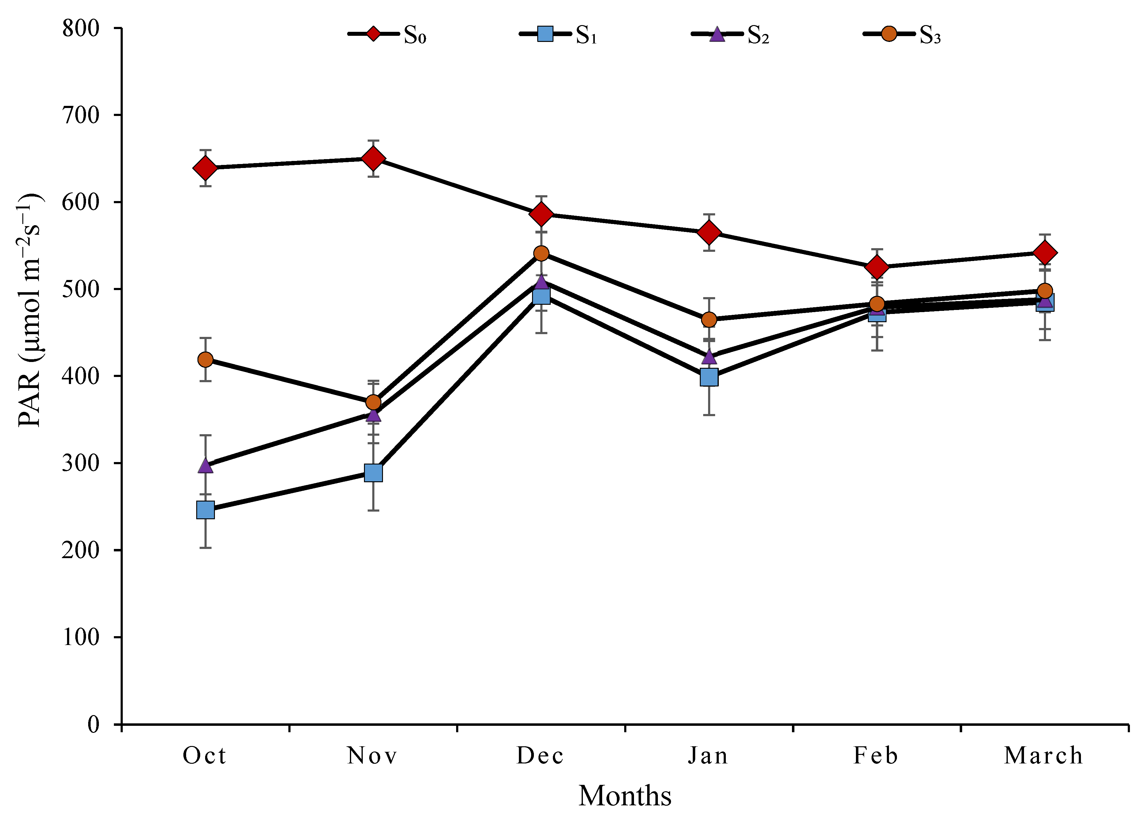
3.4. Photosynthetic Active Radiation (µmol m⁻² s⁻¹)

Photosynthetic active radiation (PAR) gradually increased with increasing tree spacing (Figure 2). The maximum value (584.5 µmol m⁻² s⁻¹) of PAR was observed in S₀ (open), while in agroforestry interventions, it ranged between 397.5 and 462.68 µmol m⁻² s⁻¹.

3.5. Soil Physicochemical Properties

The data in

Table 5. Effects of tree spacing and nutrient sources on soil physicochemical properties.

Treatment	pH	EC (dS m−1)	Bulk Density (gm cm−3)	Organic Carbon (%)	SOC (Mg ha−1)	Available N (kg ha−1)	Available P (kg ha−1)	Available K (kg ha−1)
Tree Spacing (A)
S0 (Open)	7.20 (+) 0.30	0.170 (+) 0.02	1.26 (−) 0.01	1.65 (+) 0.55	31.15 (+) 10.19	303.11 (+) 34.81	51.29 b (+) 20.79	198.99 b (+) 8.09
S1 (10 m × 1 m)	7.16 (+) 0.34	0.174 (+) 0.024	1.25 (−) 0.006	1.67 (+) 0.57	31.27 (+) 10.48	333.24 a (+) 24.94	59.74 ab (+) 24.64	202.91 b (+) 10.11
S2 (10 m × 2 m)	7.12 (+) 0.23	0.175 (+) 0.015	1.23 (−) 0.005	1.76 (+) 0.62	32.55(+) 11.35	334.30 a (+) 52.70	65.75 a (+) 25.05	239.34 ab (+) 42.44
S3 (10 m × 3 m)	7.08 (+) 0.35	0.207 (+) 0.050	1.22 (−) 0.024	1.77 (+) 0.57	32.25 (+) 9.93	348.82 a (+) 58.02	69.61 a(+) 23.31	253.03 a (+) 52.13
CD0.05	NS	NS	NS	NS	NS	29.93	12.64	41.99
Fertilizer Treatment (B)
T0 (Control)	7.13 (+) 0.29	0.153 (−) 0.002	1.27 a (+) 0.01	1.56 (+) 0.43	29.64 (+)8.33	298.30 (+) 11.05	51.14 c(+) 12.99	186.82 c (−) 8.56
T1 (FYM)	7.11 (+) 0.28	0.211 (+) 0.057	1.21 b (−) 0.05	1.90 (+) 0.76	34.32 (+) 13.0	347.82 a (+) 60.57	72.67 a(+) 34.52	252.43 a (+) 57.06
T2 (VC)	7.14 (+) 0.30	0.172 (+) 0.018	1.24 ab (−) 0.008	1.73 (+) 0.59	32.09 (+) 10.77	341.63 a (+) 54.38	62.90 b (+) 24.75	200.18 bc (+) 4.80
T3 (Jeevamrut)	7.20 (+) 0.36	0.164 (+) 0.010	1.26 a (+) 0.005	1.64 (+) 0.51	30.77 (+) 9.45	327.84 a (+) 40.59	53.47 c (+) 15.32	197.32 b (+) 1.94
T4 (FYM+VC)	7.11(+) 0.27	0.189 (+) 0.035	1.24 ab (−) 0.01	1.74 (+) 0.60	32.17 (+) 10.85	333.13 a (+) 45.88	65.28 ab (+) 27.13	266.05 a (+) 70.68
T5(RDF)	7.16 (+) 0.32	0.199 (+) 0.045	1.23 b (−) 0.02	1.72 (+) 0.59	31.83 (+) 10.51	330.48 a (+) 43.23	64.13 b (+) 25.98	238.63 ab (+) 43.25
CD0.05	NS	NS	0.03	NS	NS	25.56	7.9	46.16

The mean followed by (+/−) is the change at the end of experimentation over the initial ones, where the (+) sign indicates an increase and the (−) sign indicates a decrease. The values carrying different alphabetical superscripts (^a–c) within the columns above differ significantly among themselves (p < 0.05); NS—non-significant; CD—critical difference. Here, S₀—sole cropping; tree spacing—S₁ (10 m × 1 m), S₂ (10 m × 2 m), S₃ (10 m × 3 m); fertilizer treatment—T₀—control; T₁—farmyard manure; T₂—vermicompost (VC); T₃—jeevamrut; T₄—farmyard manure + vermicompost; T₅—recommended dose of fertilizer.

indicate that the G. optiva-based AFS appreciably (p < 0.05) improved the availability of N, P, and K. The available N (348.82 kg ha⁻¹), P (69.61 kg ha⁻¹), and K (253.03 kg ha⁻¹) were significantly greater (p < 0.05) under G. optiva planted at a spacing of 10 m × 1 m than under sole cropping (open field conditions). Regardless of the agroforestry system, applying fertilizer appreciably (p < 0.05) impacted the bulk density and available N, P, and K. The highest value for bulk density (1.27 g cm⁻³) was recorded in the T₀ treatment (control), which was significantly greater than that in the T₂ treatment (FYM) alone. Compared with the control treatment, the application of fertilizer (all treatments) significantly (p < 0.05) increased the available N. The maximum levels of available N (347.82 kg ha⁻¹) and P (72.67 kg ha⁻¹) were recorded in the T₁ treatment (FYM). In contrast, the maximum available K (266.05 kg ha⁻¹) was observed in the T₄ treatment (FYM + VC), which was greater than that in the T₀ (control), T₂, and T₃ treatments. The interaction effect between the spacing and treatments was significant and had the greatest effect on the available N (403.80 kg ha⁻¹) and P (88.77 kg ha⁻¹) contents when the pea crop was intercropped at the S₃ tree spacing (10 m × 3 m) and supplied with T₁ (FYM) (Figure 3). However, the maximum available K (337.33 kg ha⁻¹) content was observed in the S₂ treatment (10 m × 2 m) and the T₁ (FYM) treatment. Moreover, there was no significant (p < 0.05) increase or decrease in the physicochemical status during the period of the investigation (Table 5). However, fertilizer application significantly (p < 0.05) influenced/altered the bulk density, OC (%), and available N, P, and K status. The bulk density increased under the T₀ control (0.01 g cm⁻³) and T₃ (jeevamrut) treatments but decreased under the other treatments—T₁, T₂, T₄, and T₅. The maximum increase in OC and available N and P was observed in treatment T₁ (FYM), while the maximum increase (70.68 kg ha⁻¹) in available K occurred in treatment T₄ (FYM + VC).

3.6. Bioeconomic Appraisal

An economic analysis of the G. optiva-based AFS (Figure 4) demonstrated that on average, net returns of 1560.76 (S₁), 1310.78 (S₂), and 1239.79 (S₃) USD ha⁻¹ yr⁻¹ were calculated for pea intercropping under G. optiva, which was 1.82–2.29 times greater than that for sole cropping (678.91 USD ha⁻¹ yr⁻¹) (Tables S1–S8). Regardless of G. optiva tree spacing, the maximum net return (1683.94 USD ha⁻¹ yr⁻¹) was achieved with the application of T₁ (FYM), followed by T₄, T₃, T₀, T₂, and T₅. The interaction effect showed maximum net returns (2046.99 USD ha⁻¹ yr⁻¹) when the pea crop was intercropped at the S₁ tree spacing (10 m × 1 m) and supplied with T₁ (FYM) (Table S9). At all spacing levels (S₁, S₂, S₃, and sole cropping), the application of FYM (T₁) resulted in greater net returns than did T₀, T₂, T₃, T₄, and T₅.

4. Discussion

4.1. Effect of Tree Density on Growth and Biomass Partitioning

The degree to which competition influences the height and shape of trees can be crucial for growing straight trees or regulating branch size. As density also affects the shape and height of trees, enhancing the initial stocking rate, i.e., the number of stems per ha, can result in greater tree height [47]. Height growth plays a key role in morphological adaptation to light competition in shaded environments [48], and plants tend to typically direct more photosynthates towards height growth rather than girth development [49]. This probably led to the increased height growth observed at shorter spacings (10 m × 1 m) compared with wider spacings (10 m × 3 m), with the opposite trend for diameter growth observed in the current investigation. Hence, trees can be managed with either closer or wider spacing, depending on the desired size of the final harvest, for instance, greater growth in height or diameter. On the other hand, trees responded well to the resources available at the widest spacing, such as better availability of soil, moisture, and light [50], which might have been responsible for improved tree growth features such as collar diameter, crown spread, and number of primary branches on a per-tree basis. Similarly, increased resource acquisition [51] and reduced above- and below-ground competition could have promoted the growth of trees with the widest spacing. Consistent with the results of this study, Chotchutima et al. [52] reported maximum diameter at the widest spacing in Leucaena trees, and Bernardo et al. [53] reported maximum diameter at the widest spacing in Eucalyptus trees. Moreover, Hein et al. [54] reported the narrowest and shortest crown of Pseudotsuga menziesii (Mirb.) Franco at the closest spacing, while Carter et al. [55] and Makinen and Hein [56] observed a greater number of branches in Douglas fir and Picea abies, consistent with the findings of the current investigation.

Among the above-ground tree components (stem, branch, and leaf), the stem contributed the most biomass, followed by the branches and leaves for all three plant spacings. A plausible reason for the observed trend of increasing biomass with increasing planting density is the different numbers of trees in each spacing. Moreover, per-tree biomass decreased at the closest spacing (S₁) but increased on a per-hectare basis because of the high stocking level (1000 trees) in S₁ (10 m × 1 m) compared with 500 trees in S₂ (10 m × 2 m) and 333 trees in S₃ (10 m × 3 m). The present findings substantiate the previous studies by Hegazy et al. [57], Benomar et al. [49], and Routray et al. [58] in Conocarpus erectus, Populus deltoides, and Acacia mangium, respectively, who also reported maximum biomass in closest spacing.

4.2. Carbon Storage and C Sequestration Potential of G. optiva AFSs

The integration of trees and shrubs in agroecosystems often creates congenial conditions and improves the productivity of AFSs, thereby providing opportunities for enhanced carbon sinks [59,60]. The present study revealed that G. optiva trees raised at different densities significantly enhanced the biomass carbon sink. The greater carbon sequestration within mixed intercropping systems than in monocropping systems can be linked to the annual inclusion of tree litter to the carbon pool, coupled with the greater growth and assimilation rates of trees relative to field crops [61]. The maximum biomass carbon density was recorded at the 10 m × 1 m spacing of G. optiva alleys. High biomass carbon density storage in closely spaced trees was also reported by Rabach et al. [62] in Calliandra in an on-station trial established at ICRAF, Kenya. Similarly, Nolte et al. [63] reported greater biomass carbon production at close spacing than at widely spaced spacing. In our investigation, biomass production ranged from 3.32 to 6.64 Mg ha⁻¹ yr⁻¹. Nair et al. [64] reported significant variability in the carbon sequestration potential of vegetation components, ranging from 0.29 Mg ha⁻¹ yr⁻¹ to 15.21 Mg ha⁻¹ yr⁻¹, in fodder bank agroforestry systems of the West African Sahel and mixed stands of Puerto Rico, respectively. Our findings align with these results, indicating that tree density is a crucial factor in the process of tree litter accumulation in the soil [65] and that higher tree density can lead to more significant carbon sequestration in the soil [66]. However, in our study, there was a slight change in the soil pool under different G. optiva densities and monocropping systems. The low carbon density and carbon sequestration rate in the soil under G. optiva planted at different densities could be attributed to the annual pollarding of trees by their highly nutritious leaves. Oelbermann and Voroney [67] reported that C sequestration in the soil is high if a significant quantity of litterfall is accredited annually. However, the variation is due to the chance deposition of leaf litter and root turnover over the years. This study highlights the importance of spatial configuration in influencing resource capture and competition in the northwestern Himalayas for sustainable agricultural practices and climate mitigation. By strategically selecting tree–crop combinations and managing spacing and canopy structure, it is possible to reduce resource-sharing competition and enhance biomass sequestration, thereby reducing atmospheric carbon dioxide levels and ensuring the long-term sustainability of agricultural practices in the region [68].

4.3. Performance of the Pea Crop

The greater plant height in agroforestry practices could be due to etiolation, where plants extend their stems to acquire light in low-irradiance environments [69,70]. In fact, Hossain et al. [71] discovered that some physiological processes usually operate under low-light conditions, resulting in better growth characteristics. Additionally, increased shade levels in agroforestry systems prolong the duration during which plants reach different phenological stages [72] and require more time for grain filling [73], thereby benefiting plants in terms of growth and yield. Factors such as enhanced vegetative growth and a greater number of branches in S₃ (10 m × 3 m) provided more sites for the translocation of photosynthates [74] and sufficient light, as well as timely lopping of the branches of trees for fodder, favoring photosynthesis and biomass partitioning to the economic parts of intercrop [75]. The high nutrient status of the soil resulted in improved growth, development, and yield characteristics of pea plants under agroforestry intervention. Zaki et al. [76] observed improved yields of peas under alley cropping with Sesbania and Leucaena compared with those under monocropping alone. Similar results for growth and productivity were proposed by Swamy et al. [77] for soybeans under tree shade, Arenas-Corraliza et al. [78] for barley and wheat under low irradiance, and Kabir et al. [79] for bell peppers under 30% shade, which validates our results.

The superiority of organic fertilizers, such as FYM, can be linked to the beneficial influence of organic manure in providing nutrients for a longer duration, particularly during the crucial stages of plant growth [80]. Unlike synthetic fertilizers that cause rapid nutrient release and depletion, organic fertilizers provide a steady nutrient supply, which is vital for better vegetative growth, culminating in higher yields. This approach could potentially enhance the healthy nutrient status of the soil by delivering optimal levels of macronutrients and micronutrients such as Zn, Cu, Fe, Mn, and Mg [81,82,83] because of the gradual decomposition process. Additionally, it could improve the soil’s physicochemical properties, including structure, porosity, and water-holding capacity, as well as its biological properties [82]. These enhancements, combined with the gradual nutrient release of organic manure, facilitate more efficient plant nutrient uptake and utilization. Similar results have been reported by Gill [84], Pandey et al. [85], Saket et al. [86], Gonmei et al. [87], Aher et al. [88], Solanki et al. [89], and Zalate and Padmani [90], who also registered higher yields with the application of organic manures. Furthermore, the application of FYM + VC may have improved pod traits by providing a sustained and synchronized supply of nutrients, potentially leading to enhanced protein synthesis and photosynthesis [91]. This conjoint application of organic manures (FYM + VC) likely promoted root proliferation and development. This improved root architecture would facilitate more efficient uptake of water and essential nutrients, which in turn would enhance food accumulation in plants [92]. The increased nutrient availability and improved plant vitality likely contributed to more robust pod development in peas, as supported by previous studies by Patil and Udmale [93], Gopinath and Mina [94], and Priyadarshini et al. [74]. Although this study was conducted over one growing season, further research on the long-term effects of different tree spacing and fertilizer treatments on soil fertility, tree growth, and overall system productivity is warranted.

4.4. Photosynthetic Active Radiation (µmol m⁻² s⁻¹)

The lower PAR under agroforestry practices is attributed to the shade produced by the tree canopy. Furthermore, PAR was at its maximum during December (541 µmol m⁻² sec⁻¹), just after the pollarding of G. optiva trees for leaves and other benefits. Pollarding, which involves removing the upper branches of trees, temporarily reduces canopy cover, allowing more sunlight to penetrate to the understory. This increase in PAR following pollarding highlights the importance of timing in agroforestry management to optimize light availability for crops. Additionally, PAR increases with greater tree spacing because wider spacing reduces canopy density and overlap, allowing more sunlight to penetrate through the gaps in the canopy, thus enhancing light availability for understory crops and improving their potential for photosynthesis and growth. Garima et al. [95] and Sharma et al. [96] reported a similar range of PAR under bamboo canopies for the mid-hill region of the northwestern Himalayas, highlighting the significant effect of canopy cover on PAR values.

4.5. Soil Physicochemical Properties

The annual deposition of leaf litter in the agroforestry system caused by G. optiva trees, and perhaps even the rapid decomposition of leaves [97], aids in the accretion of soil nutrients required for plant growth. Moreover, the presence of trees in soil systems positively influences the rhizosphere by stimulating soil organisms involved in mineralization via root exudates, leading to nutrient release and improved soil nutritional status [95,96]. Furthermore, G. optiva trees also modulate the loss of nutrients through volatilization and leaching. The current research findings are also consistent with those of Bisht et al. [98] and Kar et al. [99], who reported that the addition of nutrients (available N, P, and K) to the soil is generally higher in agroforestry systems compared with sole cropping, indicating improved nutrient availability in agroforestry.

Moreover, the reduction in bulk density could be due to increased root growth and biopores [95], increased soil microbial activity, and the external application of nutrient sources that render the soil porous and rich in carbon. Additionally, the input of organic matter to the soil leads to the addition of dry humic carbon into the soil, which helps to shorten the process of humus formation and accumulation. Furthermore, organic matter improves the synergistic interactions among soil aggregates, organic carbon, and carbon-related enzymes, favoring soil organic carbon sequestration [100]. The increased supply of soil nutrients can be linked to the fact that organic matter improves soil nutrients by reducing leaching and increasing soil biological and enzyme activities, which would have hastened the mineralization process [101]. Moreover, higher soil available nutrient levels could be a result of the gradual nutrient release from the FYM. Similar to our results, Ghosh et al. [102] reported an increase in soil nutrient availability following the incorporation of farmyard manure (FYM) in a rice–wheat cropping system. Concerning phosphorous, the parent material (dolomite limestone) of the soil [103] and the increased diversity of phosphate-solubilizing bacteria [88] act as major factors for increased phosphorous levels in the soil. It can be speculated that the interaction between these factors synergistically enhances the bioavailability of phosphorus within agroforestry systems. Edmeades [104] and Almeida et al. [105] reported that soil fertilization with animal manure can potentially supply P and K to plants. Other researchers, such as Biratu et al. [106] and Adekiya et al. [83], have reported improved soil N, P, and K contents with the inclusion of organic amendments.

4.6. Bioeconomic Appraisal

The maximum net returns from agroforestry intervention are attributed to the additional profits generated from woody components and the greater pea crop yield under pea–G. optiva intercropping systems than under monocropping systems. The incorporation of G. optiva resulted in additional sources of income through the sale of fodder and torchwood, hence improving overall profitability. In addition, their presence in the agricultural field improved the growing conditions for peas by creating a favorable microclimate, resulting in higher yields. Similarly, Kumar et al. [12] also reported greater economic returns in the intercropping of bhringraj (a medicinal plant) with G. optiva than in the monocropping of bhringraj under mid-hill conditions in the northwestern Himalayas. Kumar et al. [107], Singh et al. [108], and Chandana et al. [109] also reported that agroforestry systems are more economically feasible than monocropping systems. Hence, intercropping peas with G. optiva has greater economic potential than sole cropping.

5. Conclusions

Integrating suitable tree species at optimum tree density levels in an agroforestry framework coupled with an organic source of fertilizer can be a nature-based strategy for mitigating climate change and restoring soil health in the current scenario of environmental crisis. Planting G. optiva at a 10 m × 1 m spacing in agroforestry practices yielded markedly greater amounts of carbon stock, above-ground biomass, below-ground biomass, and total biomass than other tree densities. Similarly, the biomass carbon density (138.42 Mg ha⁻¹), as well as the rate of carbon sequestration (biomass + soil) (6.64 Mg ha⁻¹ yr⁻¹), also reached a maximum at the closest spacing. In the presence of G. optiva trees, pea and soil physicochemical qualities performed better than in the absence of these trees. Intercropping peas with G. optiva trees at a spacing of 10 m × 3 m and using FYM produced a much greater yield than the other treatments. However, parameters such as pod length, pod diameter, pod weight, number of grains per pod, and shelling percentage were greater with the application of FYM + VC. The intercropping of peas with G. optiva and the application of organic amendments (FYM, vermicompost, FYM + VC, and RDF) improved the physicochemical properties of the soil, including bulk density, organic carbon, and the availability of N, P, and K. G. optiva-based agroforestry also significantly enhanced the total carbon storage capacity, outperforming monocropping. Therefore, alleys of G. optiva established from 10 m × 1 m peas grown in an agroforestry framework along with the application of FYM are recommended for mitigating climate change, increasing pea crop productivity and soil health, and ensuring better economic returns in mid-hill Himalayan agroecosystems; however, other field crops also need to be tested at this spacing.

References

1. Singh, B.; Bishnoi, M.; Baloch, M.R.; Singh, G. Tree biomass, resource use and crop productivity in agri-horti-silvicultural Systems in the dry region of Rajasthan, India. Arch. Agron. Soil Sci. 2014, 60, 1031–1049. [Google Scholar] [CrossRef]
2. FAO. How to Feed the World in 2050. Food and Agricultural Organization of the United Nations. 2009. Available online: https://www.fao.org/fileadmin/templates/wsfs/docs/expert_paper/How_to_Feed_the_World_in_2050.pdf (accessed on 13 March 2022).
3. Licker, R.; Johnston, M.; Foley, J.A.; Barford, C.; Kucharik, C.J.; Monfreda, C.; Ramankutty, N. Mind the gap: How do climate and agricultural management explain the ‘yield gap’ of croplands around the world? Glob. Ecol. Biogeogr. 2010, 19, 769–782. [Google Scholar] [CrossRef]
4. Sharma, P.; Bhardwaj, D.R.; Singh, M.K.; Nigam, R.; Pala, N.A.; Kumar, A.; Verma, K.; Kumar, D.; Thakur, P. Geospatial technology in agroforestry: Status, prospects, and constraints. Environ. Sci. Pollut. Res. 2022, 30, 116459–116487. [Google Scholar] [CrossRef]
5. Verma, K.; Sharma, P.; Bhardwaj, D.R.; Kumar, R.; Kumar, N.M.; Singh, A.K. Land and environmental management through agriculture, forestry and other land use (AFOLU) system. In Land and Environmental Management through Forestry; Raj, A., Jhariya, M.K., Banerjee, A., Nema, S., Bargali, K., Eds.; Wiley: Hoboken, NJ, USA, 2023; pp. 247–271. [Google Scholar] [CrossRef]
6. Sharma, P.; Singh, M.; Tiwari, P.; Verma, K. Agroforestry systems: Opportunities and challenges in India. J. Pharmacogn. Phytochem. 2017, 7, 953–957. [Google Scholar]
7. Lehmann, L.M.; Smith, J.; Westaway, S.; Pisanelli, A.; Russo, G.; Borek, R.; Sandor, M.; Gliga, A.; Smith, L.; Ghaley, B.B. Productivity and economic evaluation of agroforestry systems for sustainable production of food and nonfood products. Sustainability 2020, 12, 5429. [Google Scholar] [CrossRef]
8. Bhardwaj, D.R.; Salve, A.; Kumar, J.; Kumar, A.; Sharma, P.; Kumar, D. Biomass production and carbon storage potential of agroforestry land use systems in high hills of northwestern Himalaya: An approach toward natural based climatic solution. Biomass Convers. Biorefinery 2023, 14, 18079–18092. [Google Scholar] [CrossRef]
9. Panwar, P.; Mahalingappa, D.G.; Kaushal, R.; Bhardwaj, D.R.; Chakravarty, S.; Shukla, G.; Thakur, N.S.; Chavan, S.B.; Pal, S.; Nayak, B.G.; et al. Biomass Production and Carbon Sequestration Potential of Different Agroforestry Systems in India: A Critical Review. Forests 2022, 13, 1274. [Google Scholar] [CrossRef]
10. Verma, K.; Sharma, P.; Kumar, D.; Vishwakarma, S.P.; Meena, N.K. Strategies sustainable management of agroforestry in climate change mitigation and adaptation. Int. J. Curr. Microbiol. Appl. Sci. 2021, 10, 2439–2449. [Google Scholar] [CrossRef]
11. Dufour, L.; Gosme, M.; Le Bec, J.; Dupraz, C. Does pollarding trees improve the crop yield in a mature alley-cropping agroforestry system? J. Agron. Crop Sci. 2020, 206, 640–649. [Google Scholar] [CrossRef]
12. Kumar, J.; Thakur, C.L.; Bhardwaj, D.R.; Kumar, S.; Dutt, B. Effects of integrated nutrient management on performance of bhringraj (eclipta prostrata l.) and soil fertility under the Grewia optiva Drummond. canopy in a mid-hill agroecosystem of north western Himalayas. Agrofor. Syst. 2023, 97, 711–726. [Google Scholar] [CrossRef]
13. Thevathasan, N.V.; Gordon, A.M. Ecology of tree intercropping systems in the North temperate region: Experiences from Southern Ontario, Canada. Agrofor. Syst. 2004, 61–62, 257–268. [Google Scholar] [CrossRef]
14. Nair, P.; Kumar, B.M.; Nair, V.D. An Introduction to Agroforestry: Four Decades of Scientific Developments; Springer: Berlin/Heidelberg, Germany, 2021. [Google Scholar]
15. Navale, M.R.; Bhardwaj, D.R.; Bishist, R.; Thakur, C.L.; Sharma, S.; Sharma, P.; Kumar, D.; Probo, M. Seasonal variations in the nutritive value of fifteen multipurpose fodder tree species: A case study of northwestern Himalayan mid-hills. PLoS ONE 2022, 17, e0276689. [Google Scholar] [CrossRef]
16. IGFRI. Vision 2050. 2013. Available online: https://www.igfri.res.in/2013/Vision-2050.pdf (accessed on 26 March 2022).
17. Khybri, M.L.; Gupta, R.K.; Ram, S.; Tomar, H.P.S. Crop yields of rice and wheat grown in rotation as intercrops with three tree species in the outer hills of western Himalaya. Agrofor. Syst. 1992, 17, 193–204. [Google Scholar] [CrossRef]
18. Francis, C.; Lieblein, G.; Gliessman, S.; Breland, T.A.; Creamer, N.; Harwood, R.; Salomonsson, L.; Helenius, J.; Rickerl, D.; Salvador, R.; et al. Agroecology: The ecology of food systems. J. Sustain. Agric. 2003, 22, 99–118. [Google Scholar] [CrossRef]
19. Pantera, A.; Mosquera-Losada, M.R.; Herzog, F.; Den Herder, M. Agroforestry and the environment. Agrofor. Syst. 2021, 95, 767–774. [Google Scholar] [CrossRef]
20. Wezel, A.; Casagrande, M.; Celette, F.; Vian, J.-F.; Ferrer, A.; Peigné, J. Agroecological practices for sustainable agriculture. A review. Agron. Sustain. Dev. 2014, 34, 1–20. [Google Scholar] [CrossRef]
21. Migliorini, P.; Wezel, A. Converging and diverging principles and practices of organic agriculture regulations and agroecology. A review. Agron. Sustain. Dev. 2017, 37, 63. [Google Scholar] [CrossRef]
22. Urra, J.; Alkorta, I.; Garbisu, C. Potential benefits and risks for soil health derived from the use of organic amendments in agriculture. Agronomy 2019, 9, 542. [Google Scholar] [CrossRef]
23. De Candolle, A. Origin of Cultivated Plants.; Honfer publishing Company: New York, NY, USA, 1886. [Google Scholar]
24. Kumari, A.; Singh, O.N.; Kumar, R. Effect of integrated nutrient management on growth, seed yield and economics of field pea (Pisum sativum L.) and soil fertility changes. J. Food Legum. 2012, 25, 121–124. [Google Scholar]
25. Rajput, R.; Khushwah, S. Effect of integrated nutrient management on yield of pea (Pisum sativum). Legume Res. 2005, 28, 231–232. [Google Scholar]
26. Bijalwan, A.; Dobriyal, M.J.R. Productivity of wheat (Triticum aestivum) as intercrop in Grewia optiva based traditional agroforestry system along altitudinal gradient and aspect in mid hills of Garhwal Himalaya, India. Am. J. Environ. Prot. 2014, 2, 89–94. [Google Scholar] [CrossRef]
27. Zubay, P.; Kunzelmann, J.; Ittzés, A.; Németh Zámboriné, É.; Szabó, K. Allelopathic effects of leachates of Juglans regia L., Populus tremula L. and Juglone on germination of temperate zone cultivated medicinal and aromatic plants. Agrofor. Syst. 2021, 95, 431–442. [Google Scholar] [CrossRef]
28. Verma, K.; Prasad, S.K.; Singh, M.K.; Sharma, P. Assessment of agronomic zinc biofortification of alley cropped pearl millet. Bangladesh J. Bot. 2023, 52, 203–209. [Google Scholar] [CrossRef]
29. Verma, K.; Prasad, S.; Singh, M.; Sharma, P. Response of alley-cropped pearl millet (Pennisetum Glaucum) to Nitrogen and Zinc schedules under semiarid regions. Indian J. Agron. 2023, 68, 105–109. [Google Scholar] [CrossRef]
30. Chaturvedi, O.; Handa, A.; Kaushal, R.; Uthappa, A.; Sarvade, S.; Panwar, P. Biomass production and carbon sequestration through agroforestry. Range Manag. Agrofor. 2016, 37, 116–127. [Google Scholar]
31. Verma, T.; Bhardwaj, D.R.; Sharma, U.; Sharma, P.; Kumar, D.; Kumar, A.; Kumar, A. Agroforestry systems in the mid-hills of the northwestern Himalaya: A sustainable pathway to improved soil health and climate resilience. J. Environ. Manag. 2023, 348, 119264. [Google Scholar] [CrossRef]
32. Bhutia, P.L.; Thakur, C.L.; Sarvade, S.; Bhardwaj, D.R.; Kaushal, R.; Bhutia, K.G. Varietal performance of pea (Pisum Sativum L.) under peach-based agroforestry system in mid hill conditions of Himachal Pradesh. Indian J. Agrofor. 2015, 17, 14–17. [Google Scholar]
33. FSI. Volume Equations for Forests of India, Nepal and Bhutan; FSI: Arlington, VA, USA, 1996. [Google Scholar]
34. Chidumayo, E.N. Above-ground woody biomass structure and productivity in a Zambezian woodland. For. Ecol. Manag. 1990, 36, 33–46. [Google Scholar] [CrossRef]
35. Smith, D.M. Maximum Moisture Content Method for Determining Specific Gravity of Small Wood Samples; No. Report 2014; U.S. Department of Agriculture: Washington, DC, USA, 1954. [Google Scholar]
36. IPCC. Good Practice Guidance for Land Use, Land-Use Change and Forestry; Institute for Global Environmental Strategies (IGES) for the IPCC: Arlington, VA, USA, 2003. [Google Scholar]
37. Cairns, M.A.; Brown, S.; Helmer, E.H.; Baumgardner, G.A. Root biomass allocation in the world’s upland forests. Oecologia 1997, 111, 1–11. [Google Scholar] [CrossRef]
38. Mokany, K.; Raison, R.J.; Prokushkin, A.S. Critical analysis of root: Shoot ratios in terrestrial biomes. Glob. Change Biol. 2006, 12, 84–96. [Google Scholar] [CrossRef]
39. Nelson, D.W.; Sommers, L.E. Total Carbon, Organic Carbon, and Organic Matter. In SSSA Book Series; Sparks, D.L., Page, A.L., Helmke, P.A., Loeppert, R.H., Soltanpour, P.N., Tabatabai, M.A., Johnston, C.T., Sumner, M.E., Eds.; Soil Science Society of America, American Society of Agronomy: Madison, WI, USA, 1996; pp. 961–1010. [Google Scholar] [CrossRef]
40. Rogelj, J.; Schaeffer, M.; Meinshausen, M.; Knutti, R.; Alcamo, J.; Riahi, K.; Hare, W. Zero emission targets as long-term global goals for climate protection. Environ. Res. Lett. 2015, 10, 105007. [Google Scholar] [CrossRef]
41. Jackson, M. Soil Chemical Analysis Prentice; Hall India Priv. Limited: New Delhi, India, 1967; p. 498. [Google Scholar]
42. Walkley, A.; Black, C. An examination of digestion of method for determining soil organic matter and a proposed modification of the chromic and titration method. Soil Sci. 1934, 37, 29–38. [Google Scholar] [CrossRef]
43. Subbiah, B.V.; Asija, G.L. A rapid procedure for the determination of available nitrogen in the soil. Curr. Sci. 1956, 25, 259–260. [Google Scholar]
44. Olsen, S.R.; Cole, C.V.; Watanabe, F.S.; Dean, L.A. Estimation of Available Phosphorus in Soils by Extraction with Sodium Bicarbonate; United States Department of Agriculture Circular 19: Washington, DC, USA, 1954; p. 939. [Google Scholar]
45. Merwin, H.D.; Peech, M. Exchangeability of soil potassium in sand, silt and clay fractions as influenced by the nature of the complimentary exchangeable cations. Soil Sci. Soc. Am. Proc. 1950, 15, 125–128. [Google Scholar] [CrossRef]
46. Gomez, L.; Gomez, A. Statistical Procedures for Agricultural Research; John Wiley and Sons: Singapore, 1984. [Google Scholar]
47. Antón-Fernández, C.; Burkhart, H.E.; Strub, M.; Amateis, R.L. Effects of initial spacing on height development of loblolly pine. For. Sci. 2011, 57, 201–211. [Google Scholar] [CrossRef]
48. Lanner, R.M. On the insensitivity of height growth to spacing. For. Ecol. Manag. 1985, 13, 143–148. [Google Scholar] [CrossRef]
49. Benomar, L.; DesRochers, A.; Larocque, G.R. The effects of spacing on growth, morphology and biomass production and allocation in two hybrid poplar clones growing in the boreal region of Canada. Trees 2012, 26, 939–949. [Google Scholar] [CrossRef]
50. Prasad, J.V.N.S.; Korwar, G.R.; Rao, K.V.; Mandal, U.K.; Rao, G.R.; Srinivas, I.; Venkateswarlu, B.; Rao, S.N.; Kulkarni, H.D. Optimum stand density of Leucaena Leucocephala for wood production in Andhra Pradesh, Southern India. Biomass Bioenergy 2011, 35, 227–235. [Google Scholar] [CrossRef]
51. Manasa, P.C.; Salimath, K.S.; Hegde, R.; Amanulla, B.; Kumar, C. Biomass and Carbon stock in forest plantations: Manipulation through spacing. J. Tree Sci. 2016, 35, 71. [Google Scholar] [CrossRef]
52. Chotchutima, S.; Kangvansaichol, K.; Tudsri, S.; Sripichitt, P. Effect of spacing on growth, biomass yield and quality of Leucaena leucocephala for renewable energy in Thailand. J. Sustain. Bioenergy Syst. 2013, 03, 48–56. [Google Scholar] [CrossRef]
53. Bernardo, A.L.; Reis, M.G.F.; Reis, G.G.; Harrison, R.B.; Firme, D.J. Effect of spacing on growth and biomass distribution in Eucalyptus camaldulensis, E. pellita and E. urophylla plantations in southeastern Brazil. For. Ecol. Manag. 1998, 104, 1–13. [Google Scholar] [CrossRef]
54. Hein, S.; Weiskittel, A.R.; Kohnle, U. Effect of wide spacing on tree growth, branch and sapwood properties of young Douglas-fir [Pseudotsuga Menziesii (Mirb.) Franco] in southwestern Germany. Eur. J. For. Res. 2008, 127, 481–493. [Google Scholar] [CrossRef]
55. Carter, R.E.; Miller, I.M.; Klinka, K. Relationships between growth form and stand density in immature Douglas-fir. For. Chron. 1986, 62, 440–445. [Google Scholar] [CrossRef]
56. Mäkinen, H.; Hein, S. Effect of wide spacing on increment and branch properties of young Norway spruce. Eur. J. For. Res. 2006, 125, 239–248. [Google Scholar] [CrossRef]
57. Hegazy, S.; Aref, I.; Al-Mefarrej, H.; Hamad & El-Juhany, L. Effect of spacing on the biomass production and allocation in Conocarpus erectus L. trees grown in Riyadh, Saudi Arabia. Saudi J. Biol. Sci. 2008, 15, 315–322. [Google Scholar]
58. Routray, S.; Bhol, N.; Nayak, R.; Mohapatra, S. Biomass production and carbon sequestraion of mangium (Acacia Mangium Willd.) under varying plant spacing. Indian For. 2018, 144, 527–531. [Google Scholar]
59. Albrecht, A.; Kandji, S.T. Carbon sequestration in tropical agroforestry systems. Agric. Ecosyst. Environ. 2003, 99, 15–27. [Google Scholar] [CrossRef]
60. Sharma, R.; Pradhan, L.; Kumari, M.; Bhattacharya, P. Assessment of Carbon Sequestration Potential of Tree Species in Amity University Campus Noida. Environ. Sci. Proc. 2021, 3, 52. [Google Scholar] [CrossRef]
61. Peichl, M.; Thevathasan, N.V.; Gordon, A.M.; Huss, J.; Abohassan, R.A. Carbon sequestration potentials in temperate tree-based intercropping systems, southern Ontario, Canada. Agrofor. Syst. 2006, 66, 243–257. [Google Scholar] [CrossRef]
62. Rabach, V.O.; Koske, J.; Muna, M.M.; Muriuki, J.; Ngare, I.O. Carbon sequestration in agroforestry systems between conservation agriculture and conventional practice in the Asal area of Machakos County, Kenya. J. Appl. Agric. Sci. Technol. 2020, 4, 118–133. [Google Scholar] [CrossRef]
63. Nolte, C.; Tiki-Manga, T.; Badjel-Badjel, S.; Gockowski, J.; Hauser, S.; Weise, S.F. Effects of calliandra planting pattern on biomass production and nutrient accumulation in planted fallows of southern Cameroon. For. Ecol. Manag. 2003, 179, 535–545. [Google Scholar] [CrossRef]
64. Nair, P.K.R.; Nair, V.D.; Mohan Kumar, B.; Showalter, J.M. Carbon Sequestration in Agroforestry Systems. In Advances in Agronomy; Elsevier: Amsterdam, The Netherlands, 2010; Volume 108, pp. 237–307. [Google Scholar] [CrossRef]
65. Fernández-Núñez, E.; Rigueiro-Rodríguez, A.; Mosquera-Losada, M.R. Carbon allocation dynamics one decade after afforestation with Pinus radiata D. Don and Betula alba L. under two stand densities in NW Spain. Ecol. Eng. 2010, 36, 876–890. [Google Scholar] [CrossRef]
66. Islam, M.; Dey, A.; Rahman, M. Effect of tree diversity on soil organic carbon content in the homegarden agroforestry system of northeastern Bangladesh. Small-Scale For. 2015, 14, 91–101. [Google Scholar] [CrossRef]
67. Oelbermann, M.; Voroney, R.P. Carbon and nitrogen in a temperate agroforestry system: Using stable isotopes as a tool to understand soil dynamics. Ecol. Eng. 2007, 29, 342–349. [Google Scholar] [CrossRef]
68. Luedeling, E.; Kindt, R.; Huth, N.I.; Koenig, K. Agroforestry systems in a changing climate—Challenges in projecting future performance. Curr. Opin. Environ. Sustain. 2014, 6, 1–7. [Google Scholar] [CrossRef]
69. Zhang, J.; Smith, D.; Liu, W.; Chen, X.; Yeng, W. Effects of shade and drought stress on soybean hormones and yield of main-stem and branch. Afr. J. Biotechnol. 2011, 10, 14392–14398. [Google Scholar] [CrossRef]
70. Rizwan, M.; Rauf, A.; Rahmawaty, E.N.A. Physiology Response of Soybean Variety to Various Types of Shading in Agroforestry System. In Proceedings of the 7th International Conference on Multidisciplinary Research, Medan, Indonesia, 5–6 September 2018; SCITEPRESS—Science and Technology Publications: Sumatera Utara, Indonesia, 2018; pp. 225–230. [Google Scholar] [CrossRef]
71. Hossain, M.A.; Akamine, H.; Ishimine, Y.; Teruya, R.; Aniya, Y.; Yamawaki, K. Effects of relative light intensity on the growth, yield and curcumin content of turmeric (Curcuma Longa L.) in Okinawa, Japan. Plant Prod. Sci. 2009, 12, 29–36. [Google Scholar] [CrossRef]
72. Kumar, R.; Sharma, S.; Ramesh, K.; Singh, B. Effects of shade regimes and planting geometry on growth, yield and quality of the natural sweetener plant stevia (Stevia Rebaudiana Bertoni) in northwestern Himalaya. Arch. Agron. Soil Sci. 2013, 59, 963–979. [Google Scholar] [CrossRef]
73. Hadi, H.; Ghassemi-Golez, K.; Khoei, F.R.; Valizadeh, M.; Shakib, M.R. Response of common bean (Phaseolus vulgaris L.) to different levels of shade. J. Agron. 2006, 5, 595–599. [Google Scholar] [CrossRef]
74. Priyadharshini, A.; Singh, V.; Tiwari, D.; Budige, K.; Mahesh, K. Influence of spacing and organic manures on growth, yield and economics of mung bean (Vigna radiata L.). Biol. Forum–An Int. J. 2021, 13, 617–621. [Google Scholar]
75. Khalid, M.H.B.; Raza, M.A.; Yu, H.Q.; Sun, F.A.; Zhang, Y.Y.; Lu, F.Z.; Si, L.; Iqbal, N.; Khan, I.; Fu, F.L.; et al. Effect of shade treatments on morphology, photosynthetic and chlorophyll fluorescence characteristics of soybean (Glycine Max L. Merr.). Appl. Ecol. Environ. Res. 2019, 17, 2551–2569. [Google Scholar] [CrossRef]
76. Zaki, H.; Mahmoud, A.; Abd El-Ati, Y.; Hammad, A.; Sayed, R. Studies on pea (Pisum sativum L.) growth and productivity under agroforestry system: 2. Yield and seed quality of pea under alley cropping system with two types of trees. J. Basic Appl. Res. 2017, 3, 1–9. [Google Scholar]
77. Swamy, S.L.; Mishra, A.; Puri, S. Biomass production and root distribution of Gmelina arborea under an agrisilvicultre system in subhumid tropics of Central India. New For. 2003, 26, 167–186. [Google Scholar] [CrossRef]
78. Arenas-Corraliza, M.G.; Rolo, V.; López-Díaz, M.L.; Moreno, G. Wheat and barley can increase grain yield in shade through acclimation of physiological and morphological traits in Mediterranean conditions. Sci. Rep. 2019, 9, 9547. [Google Scholar] [CrossRef] [PubMed]
79. Kabir, M.Y.; Díaz-Pérez, J.C.; Nambeesan, S.U. Effect of shade levels on plant growth, physiology, and fruit yield in bell pepper (Capsicum annuum L.). Acta Hortic. 2020, 1268, 311–318. [Google Scholar] [CrossRef]
80. Paramesh, V.; Kumar, P.; Bhagat, T.; Nath, A.J.; Manohara, K.K.; Das, B.; Desai, B.F.; Jha, P.K.; Prasad, P.V.V. Integrated Nutrient Management Enhances Yield, Improves Soil Quality, and Conserves Energy under the Lowland Rice–Rice Cropping System. Agronomy 2023, 13, 1557. [Google Scholar] [CrossRef]
81. Chaudhary, M.; Narwal, R.P. Effect of long-term application of farmyard manure on soil micronutrient status. Arch. Agron. Soil Sci. 2005, 51, 351–359. [Google Scholar] [CrossRef]
82. Premsekhar, M.; Rajashree, V. Influence of organic manures on growth, yield and quality of okra. Am.-Eurasian J. Sustain. Agric. 2009, 3, 6–8. [Google Scholar]
83. Adekiya, A.O.; Ejue, W.S.; Olayanju, A.; Dunsin, O.; Aboyeji, C.M.; Aremu, C.; Adegbite, K.; Akinpelu, O. Different organic manure sources and npk fertilizer on soil chemical properties, growth, yield and quality of okra. Sci. Rep. 2020, 10, 16083. [Google Scholar] [CrossRef]
84. Gill, B.; Randhawa, R.; Randhawa, G.; Singh, J. Response of turmeric (Curcuma longa L.) to nitrogen in relation to application of farmyard manure and straw mulch. J. Spices Aromat. Crops 1999, 8, 211–214. [Google Scholar]
85. Pandey, A.K.; Gopinath, K.; Chattacharya, P.; Hooda, K.; Sushil, S.; Kundu, S.; Selvakumar, G. Effect of source and rate of organic manures on yield attributes, pod yield and economics of organic garden pea (Pisum Sativum Subsp Hortense) in north west Himalaya. Indian J. Agric. Sci. 2006, 76, 230–234. [Google Scholar]
86. Saket, S.; Singh, S.; Namdeo, K.; Parihar, S. Effect of organic and inorganic fertilizers on yield, quality and nutrients uptake of lentil. Ann. Plant Soil Res. 2014, 16, 238–241. [Google Scholar]
87. Gonmei, L.; Umrao, R.; Ramchandra, V. Effect of different types of organic manure on the growth and yield of pea (Pisum sativum) under Jatropha curcas based agroforestry system. Int. J. Multidiscip. Res. Dev. 2018, 5, 157–159. [Google Scholar]
88. Aher, S.B.; Lakaria, B.L.; Kaleshananda, S.; Singh, A.B.; Ramana, S.; Ramesh, K.; Thakur, J.K. Effect of organic farming practices on soil and performance of soybean (Glycine max) under semiarid tropical conditions in Central India. J. Appl. Nat. Sci. 2015, 7, 67–71. [Google Scholar] [CrossRef]
89. Solanki, R.; Bhalu, V.; Jadav, K. Organic farming approach for sustaining productivity of rainfed groundnut. Ann. Agric. Res. 2006, 27, 236–239. [Google Scholar]
90. Zalate, P.; Padmani, D. Effect of organic manure and biofertilizers on yield, harvest index, shelling percentage and quality of kharif groundnut (Arachis hypogeae L.). Int. J. Agric. Sci. 2009, 5, 417–419. [Google Scholar]
91. Babu, S.; Singh, R.; Avasthe, R.K.; Yadav, G.S.; Das, A.; Singh, V.K.; Mohapatra, K.P.; Rathore, S.S.; Chandra, P.; Kumar, A. Impact of land configuration and organic nutrient management on productivity, quality and soil properties under baby maize in eastern Himalayas. Sci. Rep. 2020, 10, 16129. [Google Scholar] [CrossRef]
92. Thongney, P.L.; Khare, N.; Rout, S.; Debbarma, R. Effect of different level of vermicompost and fym organic manure on growth and yield of cucumber intercropped with citrus based agroforestry system. Adv. Bioresearch 2020, 11, 11–20. [Google Scholar]
93. Patil, H.; Udmale, K. Response of different organic inputs on growth and yield of soybean on Inceptisol. Int. J. Recent Sci. Res. 2016, 7, 14116–14120. [Google Scholar]
94. Gopinath, K.; Mina, B. Effect of organic manures on agronomic and economic performance of garden pea (Pisum sativum) and on soil properties. Indian J. Agric. Sci. 2011, 81, 236–239. [Google Scholar]
95. Garima; Bhardwaj, D.R.; Thakur, C.L.; Kaushal, R.; Sharma, P.; Kumar, D.; Kumari, Y. Bamboo-based agroforestry system effects on soil fertility: Ginger performance in the bamboo subcanopy in the Himalayas (India). Agron. J. 2021, 113, 2832–2845. [Google Scholar] [CrossRef]
96. Sharma, U.; Bhardwaj, D.R.; Sharma, S.; Sankhyan, N.; Thakur, C.L.; Rana, N.; Sharma, S. Assessment of the efficacy of various mulch materials on improving the growth and yield of ginger (Zingiber officinale) under bamboo-based agroforestry system in NW-Himalaya. Agrofor. Syst. 2022, 96, 925–940. [Google Scholar] [CrossRef]
97. Kaushal, R.; Verma, K.; Chaturvedi, O.; Alam, N. Leaf litter decomposition and nutrient dynamics in four multipurpose tree species. Range Manag. Agrofor. 2012, 33, 20–27. [Google Scholar]
98. Bisht, N.; Sah, V.K.; Satyawali, K.; Tiwari, S. Comparison of wheat yield and soil properties under open and poplar based agroforestry system. J. Appl. Nat. Sci. 2017, 9, 1540–1543. [Google Scholar] [CrossRef]
99. Kar, S.; Pant, K.; Chandel, A.; Roshanzada, S. Trend of soil parameters under different spacings of grewia based agroforestry system in the mid hill zones of Himachal Pradesh. Int. J. Chem. Stud. 2019, 7, 1904–1907. [Google Scholar]
100. Zhao, Z.; Zhang, C.; Li, F.; Gao, S.; Zhang, J. Effect of compost and inorganic fertilizer on organic carbon and activities of carbon cycle enzymes in aggregates of an intensively cultivated Vertisol. PLoS ONE 2020, 15, e0229644. [Google Scholar] [CrossRef]
101. Albiach, R.; Canet, R.; Pomares, F.; Ingelmo, F. Microbial biomass content and enzymatic activities after the application of organic amendments to a horticultural soil. Bioresour. Technol. 2000, 75, 43–48. [Google Scholar] [CrossRef]
102. Ghosh, S.; Wilson, B.; Ghoshal, S.; Senapati, N.; Mandal, B. Organic amendments influence soil quality and carbon sequestration in the indo-gangetic plains of India. Agric. Ecosyst. Environ. 2012, 156, 134–141. [Google Scholar] [CrossRef]
103. Singh, I.; Awasthi, O.; Meena, S. Influence of tree plantation on soil physico-chemical properties in arid region. Indian J. Agrofor. 2010, 12, 42–47. [Google Scholar]
104. Edmeades, D.C. The long-term effects of manures and fertilizers on soil productivity and quality: A review. Nutr. Cycl. Agroecosystems 2003, 66, 165–180. [Google Scholar] [CrossRef]
105. Almeida, R.F.; Queiroz, I.D.S.; Mikhael, J.E.R.; Oliveira, R.C.; Borges, E.N. Enriched animal manure as a source of phosphorus in sustainable agriculture. Int. J. Recycl. Org. Waste Agric. 2019, 8, 203–210. [Google Scholar] [CrossRef]
106. Biratu, G.K.; Elias, E.; Ntawuruhunga, P. Soil fertility status of cassava fields treated by integrated application of manure and NPK fertilizer in Zambia. Environ. Syst. Res. 2019, 8, 3. [Google Scholar] [CrossRef]
107. Kumar, R.; Gupta, P.; Gulati, A. Viable agroforestry models and their economics in Yamunanagar district of Haryana and Haridwar district of Uttaranchal. Indian For. 2004, 130, 131–146. [Google Scholar]
108. Singh, D.; Kumar, R.; Walia, S.S.; Brar, A.S.; Singh, R. Productivity and economics of turmeric (Curcuma longa L.) in responseto nitrogen applied through different sources in conjunction with biofertilizer consortium. J. Appl. Nat. Sci. 2017, 9, 497–501. [Google Scholar]
109. Chandana, P.; Madhavi Lata, A.; Aariff Khan, M.A.; Krishna, A. Climate change smart option and doubling farmer’s income through melia dubia based agri-silviculture system. Curr. Sci. 2020, 118, 444. [Google Scholar] [CrossRef]
Figure 1. Representation of the experimental layout showing the planting design of pea in a G. optiva-based agroforestry system under different spacings: (a) S1—10 m × 1 m, (b) S2—10 m × 2 m, (c) S3—10 m × 3 m.
Sustainability 16 07438 g001
Figure 2. Photosynthetic active radiation (μmol m−2 s−1) of different grewia-based agroforestry systems and monocropping systems during the experimental period. Here, S0—sole cropping; tree spacing—S1 (10 m × 1 m), S2 (10 m × 2 m), S3 (10 m × 3 m).
Sustainability 16 07438 g002
Figure 3. Available chemical nutrients in the soil for different tree densities and fertilization treatments: (a) nitrogen (kg ha−1), (b) phosphorous (kg ha−1), and (c) potassium (kg ha−1). Here, S0—sole cropping; tree spacing—S1 (10 m × 1 m), S2 (10 m × 2 m), S3 (10 m × 3 m); fertilizer treatment—T0—control; T1—farmyard manure; T2—vermicompost (VC); T3−jeevamrut; T4—farmyard manure + vermicompost; T5—recommended dose of fertilizer. The values carrying different alphabetical superscripts (a, b, c, d, etc.) for the bars above differ significantly among themselves (p < 0.05). The error bars indicate the standard deviation.
Sustainability 16 07438 g003aSustainability 16 07438 g003bSustainability 16 07438 g003c
Figure 4. Bioeconomic evaluation of G. optiva-based agroforestry systems. Here, S0—sole cropping; tree spacing—S1 (10 m × 1 m), S2 (10 m × 2 m), S3 (10 m × 3 m); fertilizer treatment—T0 —control; T1—farmyard manure; T2—vermicompost (VC); T3—jeevamrut; T4—farmyard manure + vermicompost; T5—recommended dose of fertilizer.
Sustainability 16 07438 g004