Abstract
Forecasting the future levels of air pollution provides valuable information that holds importance for the general public, vulnerable populations, and policymakers. High-quality data are essential for precise and reliable forecasts and investigations of air pollution. Missing observations arise when the sensors utilized for assessing air quality parameters experience malfunctions, which result in erroneous measurements or gaps in the dataset and hinder the data quality. This research paper presents a novel approach for imputing missing values in air quality data in a univariate approach. The algorithm employs the random forest (RF) algorithm to impute missing observations in a bi-directional (forward and reverse in time) manner for air quality (particulate matter less than 2.5 μm (PM2.5)) data from the Republic of Serbia. The algorithm was evaluated against simple methods, such as the mean and median imputation methods, for missing observations over durations of 24, 48, and 72 h. The results indicate that our algorithm yielded comparable error rates to the median imputation method for all periods when imputing the PM2.5 data. Ultimately, the algorithm’s higher computational complexity proved itself as not justified considering the minimal error decrease it achieved compared with the simpler methods. However, for future improvement, additional research is needed, such as utilizing low-code machine learning libraries and time-series forecasting techniques.
Keywords:
data imputation; air quality; PM2.5; air pollution; missing observations; machine learning 1. Introduction
Air quality (AQ) is a continuous and significant factor in public health since it is associated with increased mortality [1,2], cardiovascular diseases [2], increased susceptibility to allergens [3], and respiratory illnesses [4,5,6]. Industrialization, urbanization, and population growth can all contribute to an increase in the concentration of harmful particulate matter in the air [7,8,9]. Among all the measured AQ parameters, the presence of particulate matter with a diameter less than 2.5 μm (PM2.5) is especially problematic because it can be inhaled deeply into the body through the respiratory system [10,11]. The origins of these fine particles can be attributed to a byproduct of fossil fuels burning due to the use of vehicles and the utilization of materials for home heating [12]. In highly populated regions that experience significant traffic density, having accurate information about the AQ is crucial for the proper functioning and well-being of the community.
In 2022, diseases of the circulatory system were the primary cause of death in the Republic of Serbia (RS), where they constituted 47.3% of all recorded deaths. An additional 6% of deaths were ascribed to respiratory system diseases [13]. Both of these affected groups are susceptible to heightened air pollution. Furthermore, the annual death toll due to the consequences of air pollution amounts to approximately 6 to 7 million individuals worldwide [14,15].
The adverse effects of heightened air pollution on human health are extensively documented and widely recognized. There are numerous solutions available to reduce air pollution, but the responsibility for implementing them lies with decision makers. One effective approach to address air pollution is to predict the upcoming levels of air pollution. This offers helpful insights into future air pollution levels, which can be of great significance to the general public, vulnerable populations, and policymakers. There is an abundance of literature available on the topic of predicting air quality that ranges from traditional time-series (TS) techniques to more advanced machine learning (ML) and deep learning methods.
Classical TS forecasting methods primarily utilize the auto-regressive integrated moving average (ARIMA) model [16,17] or its variant that includes the seasonal component, which is known as SARIMA [18]. Another relatively novel classical TS forecasting method is Facebook’s Prophet [18,19,20]. Both methods are traditional TS forecasting techniques that can be effectively used to predict AQ values. Additionally, ML-based methods are also extensively employed in AQ forecasting. Various ML models can be employed for this purpose, including extreme gradient boosting (XGBoost) [21], support vector regression (SVR) [21,22,23], random forest [22], and recurrent neural networks and long short-term memories [22,24]. The primary differentiation between TS forecasting methods and ML methods lies in the data requirements of each approach. Specifically, TS forecasting methods can be utilized in a univariate manner, where future values are predicted based on the past values of the modelled variable. However, ML-based methods typically require the use of additional parameters, such as meteorological, traffic, and other data, to model the target variable. In certain instances, when there is a lack of available data, this can pose a significant problem.
However, in order to achieve accurate and reliable predictions of air pollution, it is crucial to prioritize the quality of data. This applies to both traditional TS and ML methods, as data quality is the key determinant of the accuracy of forecasts.
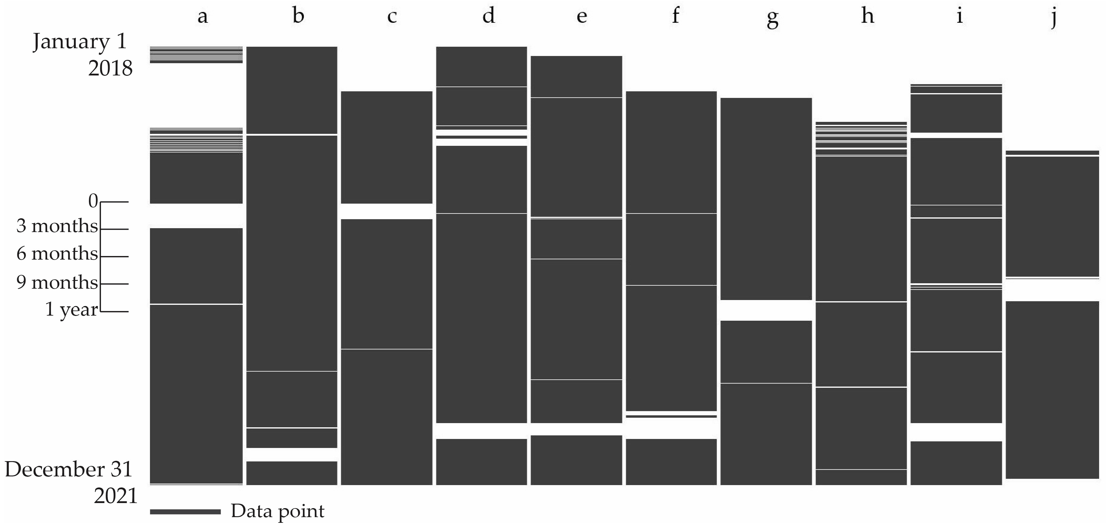
Missing observations (MOs) significantly contribute to the poor quality of AQ data. MOs occur when the sensors used to measure AQ parameters malfunction, which leads to either erroneous measurements that need to be removed by the researcher or gaps in the dataset. Figure 1 showcases 10 chosen AQ measurement stations in the RS from the Serbian Environmental Protection Agency (SEPA) network, which provides a concise representation of the seriousness of MOs over a 4-year span from 2018 to 2021. Figure 1 clearly illustrates the presence of MOs that extend over a significant duration, which presents a challenge for researchers in terms of ensuring data quality. In Figure 1, the average percentage of MOs for the AQ stations was 15.3%, with the lowest value being 3.9% (station b, Figure 1) and the highest value being 30.9% (station j, Figure 1). The possible explanation of the MOs in the SEPA network can be attributed to technical errors at the measurement sites, which occur randomly and are unrelated to the actual measured values, i.e., the data itself.

Figure 1.
Missing PM2.5 observations at selected air quality measuring stations from 1 January 2018 until 31 December 2021; a—Novi Sad Rumenačka St.; b—Belgrade Old Town; c—Belgrade New Belgrade; d—Belgrade Mostar; e—Smederevo Center; f—Obrenovac Center; g—Valjevo; h—Bor City Park; i—Kosjerić; j—Niš “Sveti Sava” Elementary School.
Figure 1 depicts the extent of MOs in AQ data that researchers must contend with. As a result, over the years, numerous AQ imputation techniques have been created, suggested, and assessed [15,25,26,27]. The mean-before-after method, which is a variation of a simple imputation method (mean imputation method), is displayed in [28]. This method takes into account two data points before and after the gap. Similar to this, bi-directional long short-term memory, which is a neural network architecture, evaluates data both before and after the MO location [29]. A comparison of other advanced methods, as well as deep learning methods, was done to analyze PM2.5 data from Peru [30]. In [31], it is displayed that Kalman smoothing on structural time series was the most effective method for data imputation using air quality data from Sydney. Furthermore, the MICE method demonstrated its advantages in the imputation of missing AQ data [32]. A method known as missforest, which is associated with the random forest algorithm, was employed to successfully impute missing AQ values for data from Kuwait [33].
The goal of this paper was to present a newly developed algorithm for imputing missing values in univariate AQ data. The decision to employ a strictly univariate approach was made due to the recognition that additional data for ML algorithms may not always be easily accessible. Therefore, having a robust, accurate, and reliable univariate method is advantageous. The algorithm is designed to determine the location of MOs, divide the data into “before” and “after” segments, and utilize the ML model to predict and fill in MOs in both forward and reverse directions in time.
2. Methods and Data
2.1. Algorithm Workflow
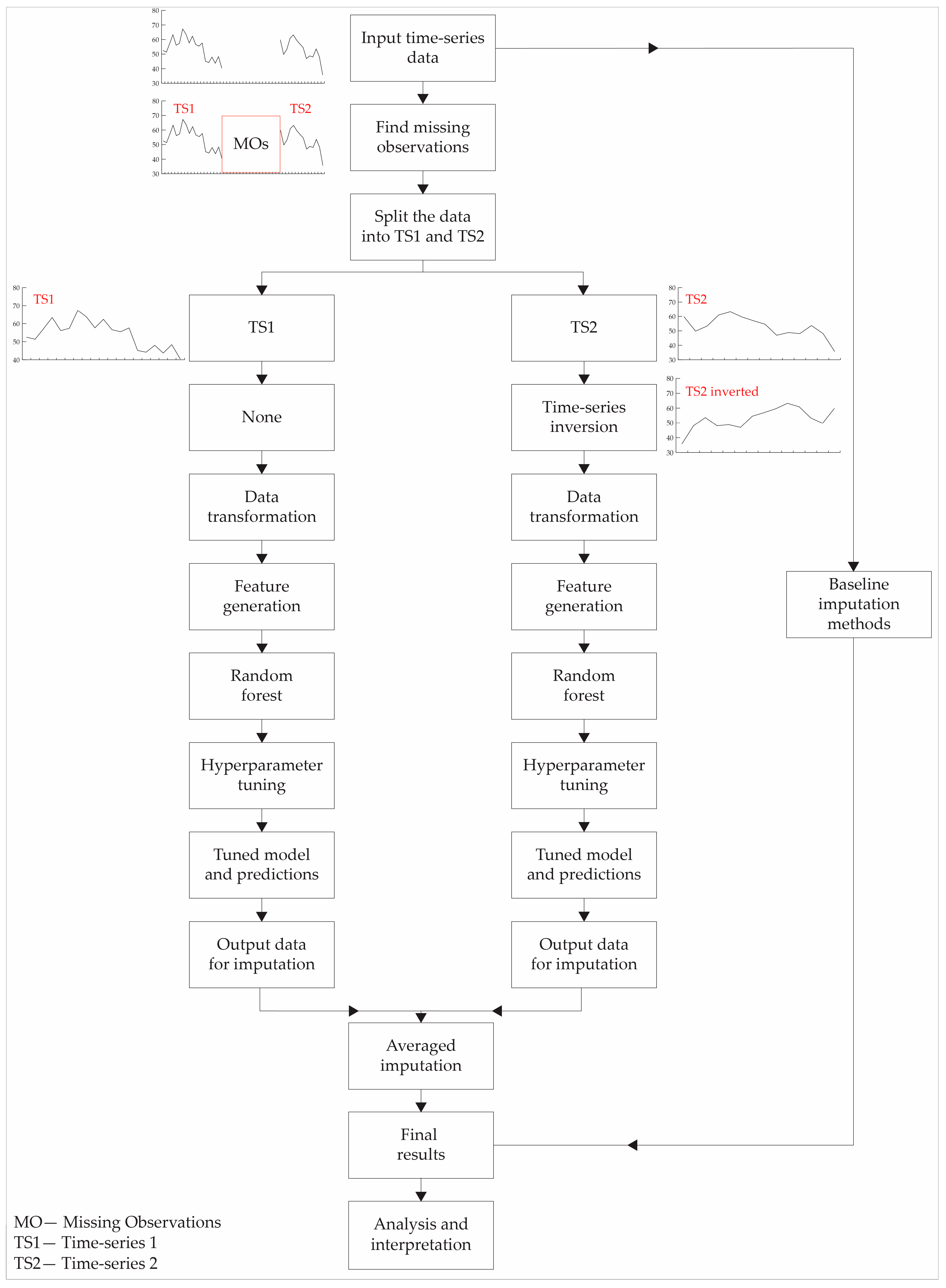
The PM2.5 data, which includes missing observations, were used as the input time series for the algorithm (Figure 2). The algorithm first identifies the gaps in the data, i.e., the MOs’ locations and sizes. Then, the input TS data are divided into two separate TSs: TS1 and TS2. TS1 is used as the TS from which the algorithm will make a forecast in the future, as is typically done in forecasting problems. On the other hand, TS2 is employed to make a forecast backward in time. To enable backward forecasting, TS2 is inverted.
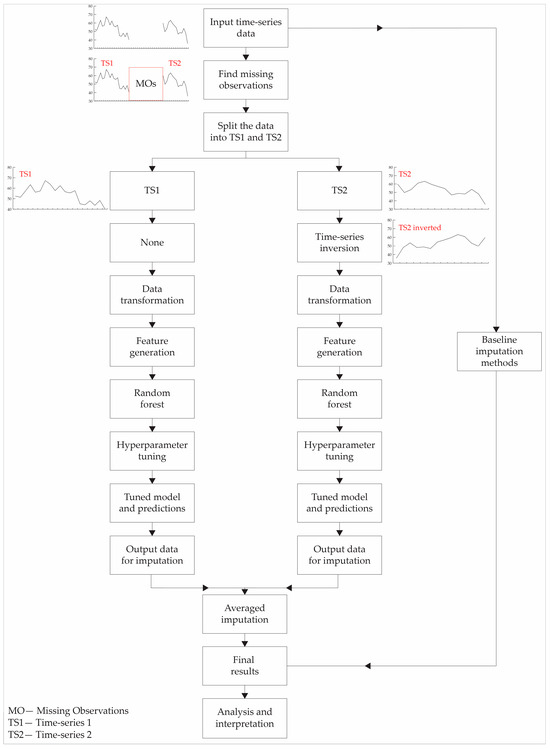
Figure 2.
Simplified air quality data imputation workflow employed in this study.
The algorithm proceeds by applying a data transformation for both TS1 and TS2 (Figure 2). The data transformation aims to reduce the range of data used for forecasting in order to simplify the data-modeling process (usually to make the data more stationary). The data transformation utilized in this research was the log transformation.
Feature discovery or feature generation is a crucial initial step in ML modeling. As previously stated, the imposed constraints of this research are that only PM2.5 data were used, without incorporating any additional data, such as meteorological conditions, traffic patterns, or other air quality parameters. Consequently, the available features that could be employed were solely the PM2.5 data. The features used in this research consisted of lagged features, i.e., look-back data, which referred to the number of data points analyzed prior to a given data point, as well as rolling window statistics, such as the mean, median, and standard deviation. The new parameters introduced into the algorithm in this step were the number of lagged features and the window size for the rolling window statistics.
Once the features are generated, the data are passed to the random forest (RF) regression model. The RF model was introduced by Breiman in 2001 [34] and has since become one of the most widely used ML algorithms. The versatility of the RF algorithm in the Earth sciences can be seen in its wide utilization across many fields, such as near-Earth physics [35,36,37,38], lithological prediction [39,40], mineral prospectivity [41,42,43], and land classification [44]. The RF model is a tree-based model that can be seen as a progression and enhancement of decision trees (DTs). DTs use a measure of homogeneity, such as the Gini index or entropy for classification tasks or the mean square error for regression tasks, to split a group of instances, where the resulting group has pure (more homogenous) target variables (the majority belonging to one class or similar range of values). This allows them to make predictions, either for classification problems (class prediction) or regression problems (number prediction). Upon receiving a new instance, the DT model assigns it to a suitable group based on the features of the given instance, and subsequently assigns the target class of the group to the new instance. DTs are simple models that were subsequently improved and surpassed by the RF model. DTs have several drawbacks, including a tendency to overfit and limited predictive power when dealing with larger and more complex datasets. However, one of their benefits is their interpretability. The RF model is a collection of DTs (ensemble model) that employs the bootstrap method with replacement to generate multiple bootstrap samples from the original dataset, which enables training more DTs. The ultimate prediction is determined through voting in classification problems or averaging in regression problems. The RF model has the number of trees as a hyperparameter, which determines the number of DTs used to train the model. The RF model offers advantages in terms of its lower susceptibility to overfitting by averaging the predictions of multiple DTs. Due to the aforementioned reasons and the ease of implementation in modern software packages and libraries, the RF model is considered an excellent initial choice when developing novel research areas.
The RF model was trained on 80% of the data, while the remaining 20% was kept aside for testing and generating values for imputation. This research employed the random search hyperparameter optimization technique, which involved testing 50 models within the range of 10 to 1000 trees. The optimized model was subsequently employed to produce values for imputation. As the model generated a new value, it was added to the feature list as an additional entry in the test set. The model then proceeded to generate another value. This process was repeated iteratively until all the data were inputted.
The identical procedure of model creation, training, tuning, and so forth that was carried out for TS1 was replicated for TS2. The TS1 and TS2 imputed values were used to calculate an average imputed value from the model, which resulted in a total of three values: forward, backward, and averaged imputation.
Alongside this process, baseline imputation methods were applied, including simple methods like mean and median imputations, where the MOs were imputed with the mean or median values of the dataset.
The error quantification for this research was done in a straightforward manner by using the absolute error (AE) and its aggregate: the mean absolute error (MAE). This research utilized multiple AQ monitoring stations, and because of that, the mean, median, minimum, and maximum MAE for each imputation method are displayed throughout this research paper.
2.2. Dataset Preparation
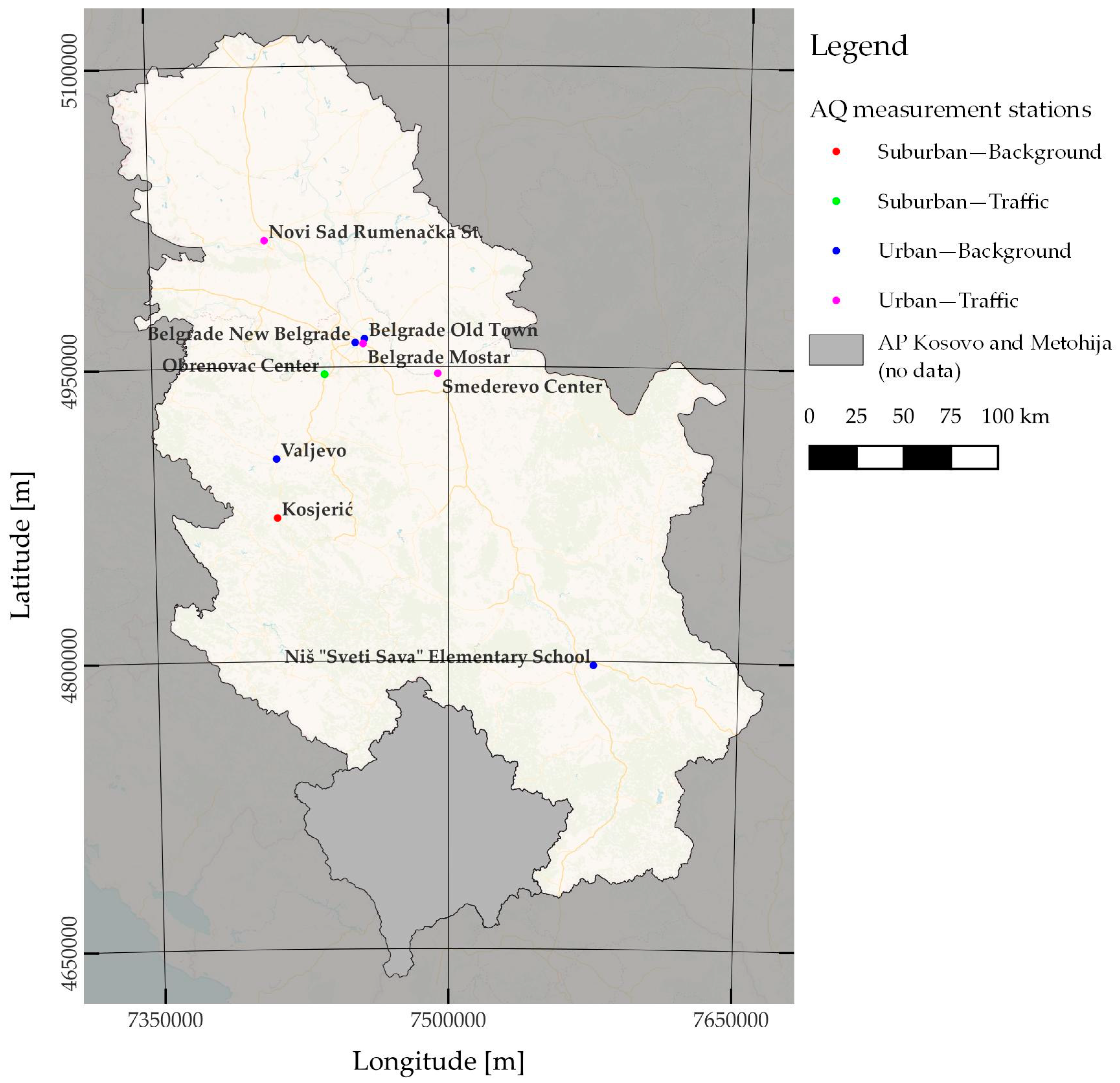
This research utilized AQ data obtained from the Serbian Environmental Protection Agency (SEPA) network. The SEPA network employs Grimm EDM 180 PM monitors [45,46] throughout the RS, which are fully automated PM monitors that operate on the principle of light scattering, i.e., an optical particle counter, for PM detection. As the AQ data collected by the SEPA network are sent to the European Environmental Agency (EEA) database, all PM measurements adhered to the standardization requirements established by the European Union and the EEA. The initial dataset comprised AQ measurements from 2018 to 2021 for different parameters, including PM2.5, PM10, SO2, CO, and NO, across different locations in the RS. The initial datasets were employed to identify the longest uninterrupted sequences of recorded PM2.5 data. Figure 3 displays a total of nine stations that were considered suitable for the current study. The durations of the consecutive data ranged from 4715 h, which was equivalent to approximately 196 consecutive measured days in Belgrade New Belgrade, to 8735 h, which was equivalent to 364 consecutive measured days in Belgrade Mostar and Old Town.
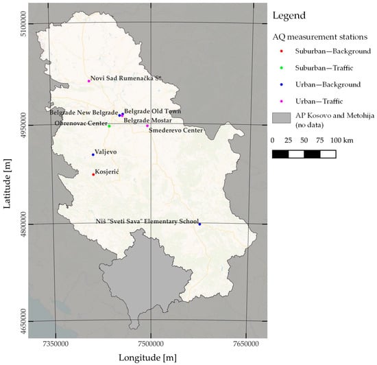
Figure 3.
Distribution of air quality monitoring stations whose data were utilized in this research across the Republic of Serbia.
The chosen PM2.5 measurement stations were distributed throughout the RS, with three located in the capital and largest city of Belgrade (Mostar, New Belgrade, and Old Town). The other two largest cities in the RS, Novi Sad and Niš, each had one selected PM2.5 measurement station. The remaining stations were spread across various localities in the RS, including Obrenovac, Valjevo, and Smederevo. In terms of the area and station classifications, the three largest cities (Belgrade, Novi Sad, and Niš) had stations situated in urban areas of the city. These stations assessed either traffic-related or background air pollution levels. The Mostar AQ station in Belgrade was situated near a prominent traffic junction that experienced heavy traffic congestion during peak hours throughout the day. Additional AQ stations were situated in suburban or urban environments and assessed either background or traffic pollutants.
Once the suitable AQ stations were determined, MOs of 24, 48, and 72 h were introduced into the TS. Random locations for the missing observations were chosen for each AQ station, which resulted in varying lengths of TS1 and TS2 in order to test the algorithm and precisely gauge its effectiveness. To quantify the error rates of the aforementioned imputation methods, the original, i.e., measured, data, which were located where the MOs were introduced, were separated and preserved for subsequent use when the models imputed the data.
A decision was made to select relatively small values of MOs (24, 48, and 72 h) and compare our algorithm with simple imputation methods, such as mean and median imputations. Additionally, the algorithm was provided with the maximum amount of available data in the given circumstances from the SEPA network. In order to provide the algorithm with optimal conditions for success, we specifically generated small MO values that yielded more data for model training and a narrower range of data that needed to be imputed. However, the decision to use mean and median imputations was made to provide the proposed algorithm with relatively simple yet widely utilized methods for comparison. Mean and median imputations, while straightforward, are suitable for data imputation in certain cases. However, they are not recommended for long sequences of data, particularly those with expected periodic patterns or variability [47,48], such as AQ data.
Furthermore, selecting the longest measured sequences of data from the SEPA network enabled the model to be in optimal conditions for demonstrating an enhancement over simple imputation methods. In other words, our algorithm was provided with the most favorable conditions in terms of the quantity of data, as well as the methods to which it was compared.
It is important to mention that certain AQ monitoring stations that were considered to be of interest (e.g., displaying high error rates and having a high variability in the data or other) were subjected to testing with alternative imputation techniques. These techniques included classic RF, which incorporates additional features, such as meteorological data and time parameters (time of day, day of week, etc.), and incorporates a classical instance-based approach and modern imputation techniques, like the iterative imputer [49] with the dataset consisting of data up to the MO location. Due to the greater number of stations and variations in the conditions and lengths of the MOs, not all stations underwent testing with alternative techniques and different features. Only a limited number of stations were selected for this purpose and are displayed in the results section.
3. Results
3.1. One Day (24 h) of Consecutive Missing Observations
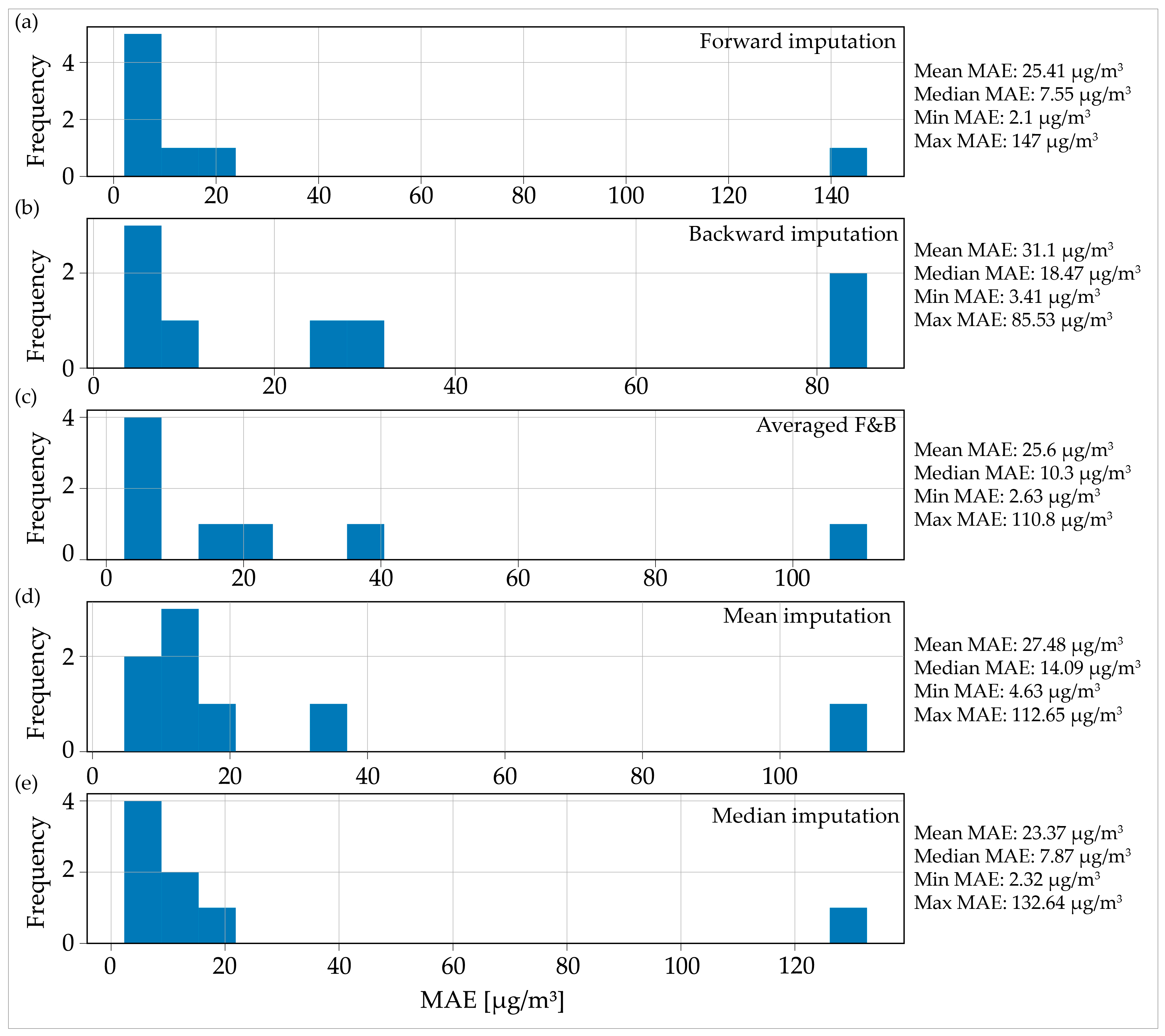
Figure 4 displays the MAE distribution for all five imputation methods used on a dataset with nine AQ measurement stations with 24 consecutive MOs. The distribution revealed the presence of a significant outlier in all the imputation methods. Specifically, for the forward imputation method (Figure 4a), the MAE for the given AQ station was approximately 147 µg/m3, while for the other methods, it ranged from 80 µg/m3 to around 100 to 120 µg/m3. This outlier skewed the average MAE calculated for all AQ stations using a given imputation method, as was evident when comparing the mean and median MAE values. When comparing the imputation methods based on the median MAE value, two methods stood out with similar minimal values: forward imputation with 7.55 µg/m3 (Figure 4a) and median imputation with 7.87 µg/m3 (Figure 4e).
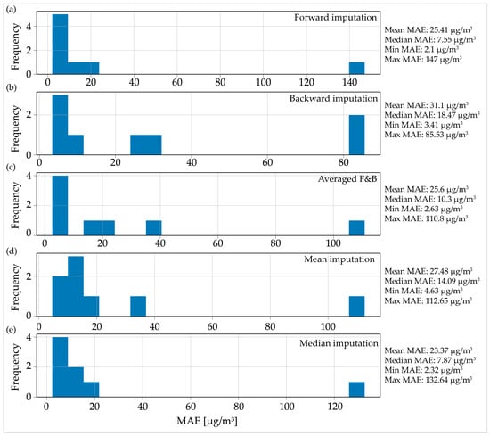
Figure 4.
Distribution of the mean absolute error for the imputed data for one day (24 h) consecutive missing observations: (a) forward imputation; (b) backward imputation; (c) averaged imputation; (d) mean imputation; (e) median imputation.
In the distributions presented in Figure 4, only eight AQ stations were included out of the total of nine that were analyzed. Upon investigating the reason for the omission of one station from the distribution, it was found that the algorithm failed to converge on one specific example, which resulted in the absence of any results for that AQ station.
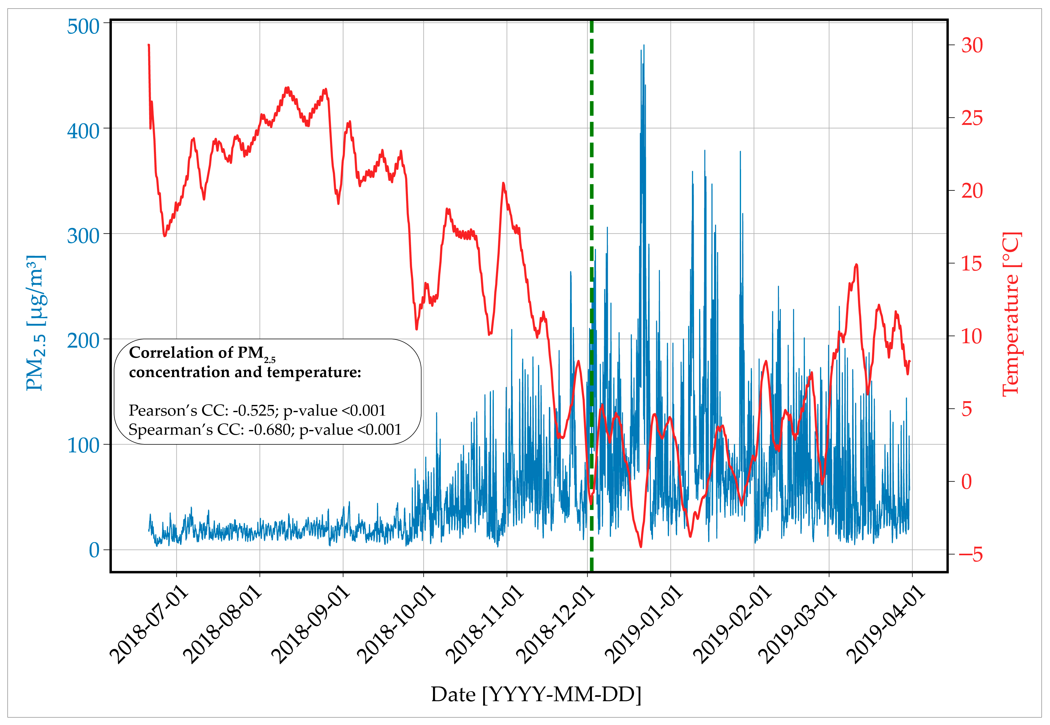
Regarding the severe outlier, all imputation methods in Figure 4 indicated that the dataset originated from the city of Valjevo. This dataset covered the period from 20 June 2018 to 31 March 2019, thus totaling 6803 h or 283 consecutive measuring days. After analyzing the Valjevo dataset, it was evident that there was a significant increase in the PM2.5 parameter values that started from the month of October (Figure 5). The locations of MOs are depicted in Figure 5 by the green dashed line, which were situated in the highly fluctuating section of the increased PM2.5 values. In the locations of the 24 h MOs, the PM2.5 values varied between approximately 80 µg/m3 and 250 µg/m3, thus exhibiting distinct peaks and lows. Due to the wide range of PM2.5 concentrations and the significant variability in these concentrations, none of the tested models were successful in accurately imputing the data with a relatively low margin of error. In addition to the higher error rate that resulted from the fluctuating levels of PM2.5, one possible explanation is that the decrease in temperature, which started in October 2018, led the residents of Valjevo to rely on wood and other combustible materials for home heating. This, in turn, contributed to the rise in ambient pollution levels. The Pearson’s and Spearman’s correlation coefficients were computed to determine the relationship between temperature and PM2.5 concentrations for the given period. The results indicate a moderate, negative correlation, meaning that as the ambient temperature decreased, the PM2.5 concentration increased and vice versa. These findings align with similar results obtained from [6].

Figure 5.
PM2.5 concentrations from 20 June 2018 to 31 March 2019 in the city of Valjevo, Republic of Serbia; blue line—PM2.5 concentrations; red line—temperature (measurement station in Belgrade, Republic of Serbia); green line—locations of missing observations.
Furthermore, two additional models, namely, the classic RF and iterative imputer, were tested on the data to evaluate their suitability for this extreme example. The two models used incorporated meteorological variables, such as the temperature, dew point, relative humidity, wind direction, wind speed, and visibility, as well as time-related variables, including time of day, day of week, and day or night classification. Both models surpassed the performance of the five previously used models; however, they still exhibited significant MAE values of 79.7 µg/m3 and 90 µg/m3 for the 24 h MO period.
3.2. Two Days (48 h) of Consecutive Missing Observations
The median imputation method yielded the lowest mean MAE value across all AQ measurement stations in the case of 48 h of MOs (Figure 6e). This was followed by the mean imputation (Figure 6d) method and the forward imputation method (Figure 6a). The application of backward imputation in this particular scenario resulted in the poorest overall performance, with an average value of 32.19 µg/m3. When examining the median MAE values, the situation varied, and the most effective method overall was forward imputation, followed by median imputation.
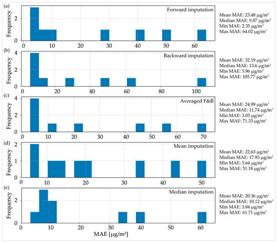
Figure 6.
Distributions of the mean absolute error for the imputed data for two days (48 h) of consecutive missing observations: (a) forward imputation; (b) backward imputation; (c) averaged imputation; (d) mean imputation; (e) median imputation.
Choosing the most efficient method for the 2-day MO case came down to deciding between forward and median imputation, as the mean and median MAE values were quite similar for both methods. However, it was crucial to consider both the computational complexity and time of the proposed method. The average duration for the proposed algorithm to generate the forward and backward data imputations was 13.21 min. However, the time split between the forward and backward imputations was not always evenly divided at 50–50%. In contrast, the median and mean imputation methods were instantaneous on modern computers. Consequently, the proposed method in this research was less effective when compared with straightforward methods for the 48 h MOs scenario.
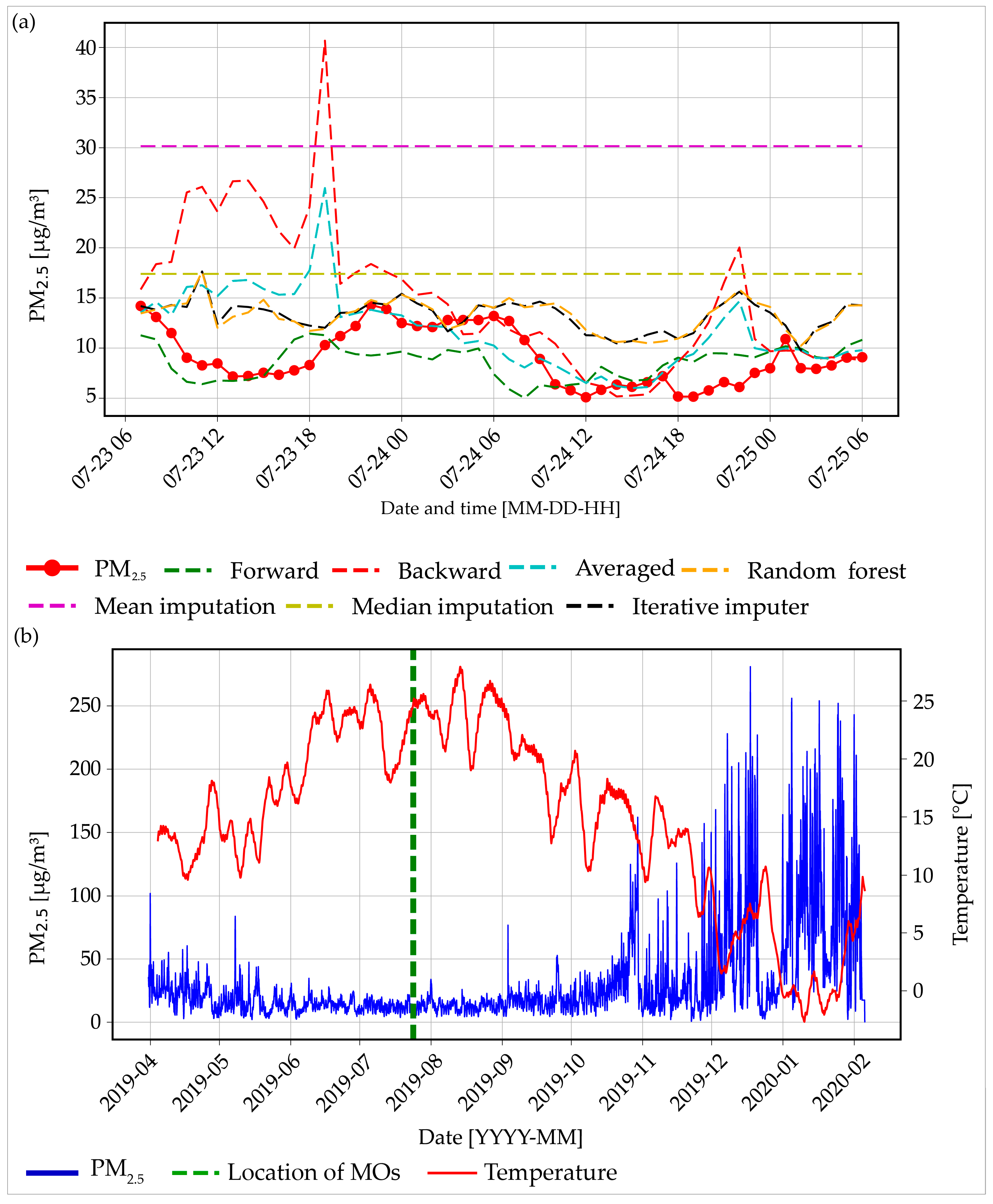
Figure 7 provides an illustration of the imputations made by different models for the Niš “Sveti Sava” elementary school example. Figure 7a displays the 48 h MO period, along with the actual PM2.5 values and imputations from different models. The proposed algorithm’s forward forecast yielded the most favorable results in terms of minimal MAE values, with a value of 2.34 µg/m3. This was closely followed by the average forecast from our algorithm (3.3 µg/m3), and then by the RF classic (4.16 µg/m3) and iterative imputer (4.17 µg/m3). When examining Figure 7b, it shows the complete PM2.5 data for the specified location, along with the temperature for the given time period and the locations of the MOs. This situation is comparable to the previous example. During the winter, the decrease in temperature led to an increase in air pollution due to the heightened usage of wood and other materials for home heating. Due to the positioning of the MOs, the backward forecast was trained using values that were higher than those used in the forward forecast. As a result, the backward forecast predicted larger values than the forward forecast and performed as the third worst model. The two models with the lowest performance were the mean imputation method, with a value of 21 µg/m3, and the median imputation method, with a value of 8.2 µg/m3. This information is noteworthy because both methods made use of the entire dataset rather than just the portion of the dataset before the locations of the MOs. Mean values are highly susceptible to the influence of outlier values, which results in the mean imputation method producing more inaccurate estimations. In contrast, median values are not affected by outliers, which leads to more accurate estimations. When a dataset has significant variations in its data values, it is more efficient to use the median instead of the mean for imputation [50].
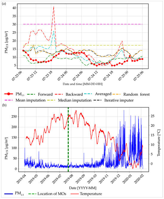
Figure 7.
(a) The 48 h missing observations period and imputed values from different models for the Niš “Sveti Sava” Elementary School example and (b) PM2.5 values for the Niš “Sveti Sava” Elementary School example with temperature values for the period.
3.3. Three Days (72 h) of Consecutive Missing Observations
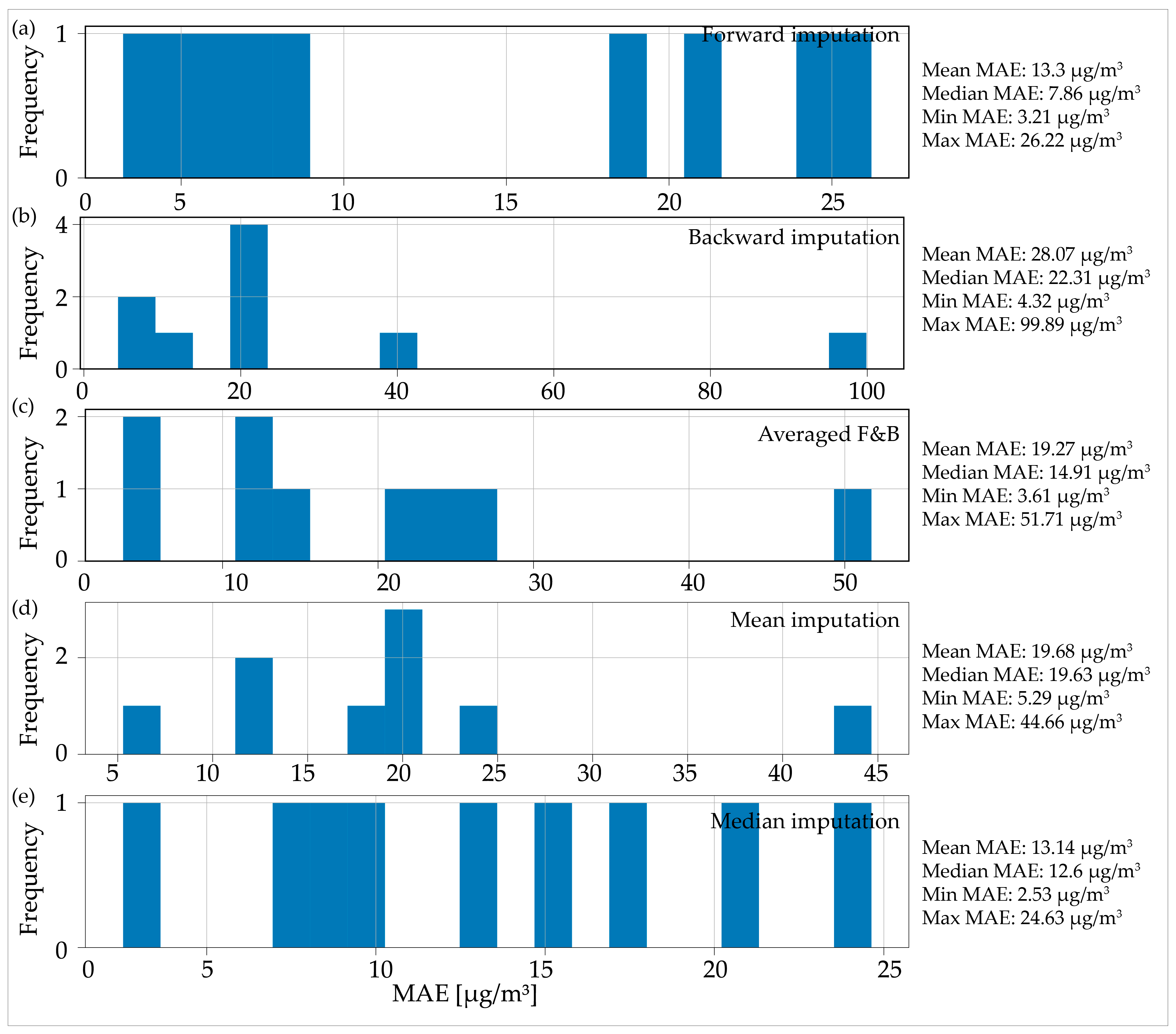
During the three days or 72 consecutive hours of MOs, the situation was analogous to the previous two examples. Figure 8 compares the forward and median imputation methods (Figure 8a,e), which were the two best overall methods. As previously mentioned, while there was a comparison between the two methods in terms of MAE values, the computational complexity and time for our method was not justified by the reduction in error estimates. In fact, the error values between a simple and instantaneous method and our method were quite similar. Furthermore, it is worth mentioning that similar to the previous example, the median imputation method yielded more accurate estimates of PM2.5 MOs compared with the mean imputation method, which showed that when having highly fluctuating data, a better choice is the median imputation method.
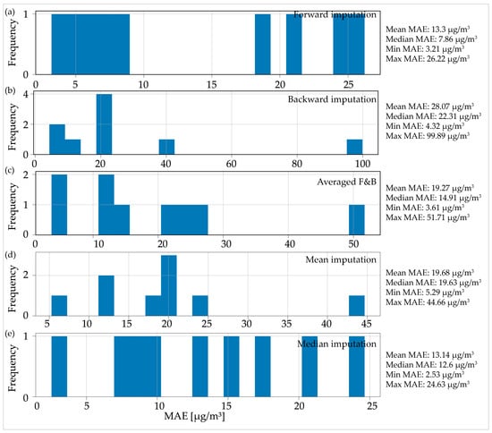
Figure 8.
Distribution of the mean absolute error for the imputed data for three days (72 h) of consecutive missing observations: (a) forward imputation; (b) backward imputation; (c) averaged imputation; (d) mean imputation; (e) median imputation.
Given the previous results and the use of the iterative imputer and classic RF up to the locations of the MOs, a different approach was taken for the example that involved three days of consecutive MOs. From the previous two examples, it was observed that there was a correlation between the temperature and the rise in PM2.5 concentrations. The correlation between the temperature and PM2.5 may be indirect due to the heating season in the RS, which begins on October 15 and ends on April 15 nationwide. This seasonal pattern could be an important feature for the model. In this example, in addition to the usual meteorological features (temperature, relative humidity, wind speed, visibility) and time features (time of day, day of week), a binary feature was included to indicate the beginning and end of the heating season in the RS. In addition, the RF model was provided with the complete dataset both before and after the locations of the MOs. The example used was Belgrade, Old Town, which included data from 31 March 2019 to 29 March 2020, thus totaling approximately 8702 consecutive measured hours (equivalent to 362 consecutive measured days). The MAE for the model that did not include the heating season feature was 11.9 µg/m3. However, when the heating season feature was included in the model, the MAE decreased to 7.8 µg/m3. In addition, the feature importance analysis determined that the heating season feature was the second most informative, after visibility and before wind speed, temperature, and relative humidity. Similarly, in the same example, the forward imputation yielded an MAE value of 7.8 µg/m3, while the backward imputation resulted in a significantly higher value of 99 µg/m3. The MAE values for the mean and median imputation models were 19.6 µg/m3 and 9.4 µg/m3, respectively.
4. Discussion
4.1. Benefits and Limitations
Considering the results presented earlier, it is necessary to address the limitations of the suggested method. While our proposed method showed favorable results in certain cases, it did not outperform simpler methods, like the mean and median imputation, overall.
Our method incurred significantly greater computational complexity and time compared with the other methods employed in this research study. The computational time for the classical, instance-based RF and iterative imputer methods, which are effective and modern techniques for data imputation, was only a few seconds. Regarding the mean and median imputation methods, as previously mentioned, the computational time was very fast, i.e., instantaneous on modern computers. Regarding our proposed method, the average computational time (on a standard home computer) for the entire algorithm was approximately 13 min. However, it is important to note that there was an unequal time distribution between the forward and backward imputations, with a 50–50% split not always being observed. Also, the computational time mentioned was achieved by allowing the algorithm to fully leverage the maximum processing capabilities. Therefore, for configurations with lower capacities, the computational time could be greater.
It is worth noting that the task of locating extended, uninterrupted sequences of measured data can be challenging. In this research paper, we selected nine SEPA AQ measurement stations that had a minimum of 4715 continuous measured data points and a maximum of 8735 continuous measured hours. This research paper presented the ideal situation for our proposed method; however, in reality, the data were characterized by a high frequency of low-duration MOs (low MO duration but high occurrence frequency) and a low frequency of high-duration MOs (high MO duration but relatively low occurrence frequency).
One more constraint of this research is that we employed the RF model to produce imputed values. The RF model possesses hyperparameters, such as the number of trees. However, our approach introduced new parameters that should be taken into account, thereby increasing the complexity of our method. The number of features in this research can be regarded as a parameter, as it is connected to lagged values and rolling window statistics. The researcher needs to determine the optimal number of lagged values to utilize, as well as the size of the rolling window. In theory, our method can be adjusted for each specific case, but this inevitably leads to a higher level of computational complexity.
Our method has a drawback in which the model generates values to sequentially fill in missing data. These generated values are then transferred to the feature set one-by-one, where they are used as data points to generate new values. This approach has a weakness in which it is trained using measured data. Introducing a synthetic data point in the feature list poses a challenge, unless that data point has a correct, i.e., expected value. In other words, the errors in our model accumulate at a faster rate compared with standard forecasting problems because each new generated data point is contingent upon the “correctness” of the previous generated data point.
Finally, it is important to acknowledge that creating a one-size-fits-all method for data imputation on AQ data is highly challenging. Another factor to consider is the increased difficulty in making the method exclusively univariate due to the presence of numerous location-specific factors (as observed with the heating period feature in this research) and the influence of multiple different factors on AQ values (traffic patterns for a given location, weather conditions, holiday season, etc.). An option is to individually address each dataset that requires data imputation by employing a variety of methods specifically tailored for the specific data at hand.
4.2. Future Perspectives
In addition to the limitations displayed earlier, there are a few noteworthy points that need to be highlighted, and further research can be expanded upon. Based on our research, we consider the proposed method of providing imputations or forecasts of MOs using two directions to be an interesting approach that deserves further investigation. In order to conduct future research, it is possible to explore two alternative methods. One possible approach is to use a low-code ML library like PyCaret [51] instead of the currently used RF method. PyCaret not only offers the ability to train, test, validate, and tune the model but also the capability to do so quickly, thereby reducing the computational time and complexity of our approach. In addition, a comparison can be made between the forward and backward imputations to determine whether divergence occurs. If it does, only one of the imputations should be used. In addition to this, another comparable approach that can be employed is the utilization of standard TS forecasting techniques, such as ARIMA or Facebook’s Prophet [52]. These methods are robust TS forecasting techniques that incorporate automated workflows for tuning parameters, specifically in the case of the ARIMA technique. Furthermore, it is worth considering a hybrid approach that combines PyCaret, which is a standard ML framework, with TS forecasting techniques. This combination has the possible potential to further improve the proposed algorithm, which we plan to conduct in the future.
Furthermore, an interesting parameter for future research in data imputation methods is the planetary boundary layer (PBL), which is a parameter that is not measured but modeled. The PBL exhibits a negative correlation with PM2.5 values [53], which makes this valuable information to include in future models. Additionally, the PBL is thinner during nighttime and in colder months. This is consistent with our observation that as the ambient temperature decreased, there was an increase in ambient AQ pollution. Future research in the field is expected to explore various perspectives in utilizing non-inherently measured data. This was because sensors often require maintenance periods, experience downtime, and may encounter malfunctions.
Finally, it is important to acknowledge for future research that AQ should be considered not only as a variable that changes over time, but also as a variable that changes both in space and time, as air pollution moves across different locations and periods, as displayed in [54,55]. Regarding data imputation methods, if the stations are in close proximity to each other, the MOs of one station can be assumed to be the same as the values of the other station in the event of a malfunction. Furthermore, studying the spatial and temporal fluctuations of air pollution is crucial, as it can provide insights into the movement of pollutants and the factors that impact their dispersion.
5. Conclusions
The matter of AQ is a crucial concern for public health that necessitates attention in vulnerable regions. Data quality is a critical aspect that includes the quantity of missing data. One possible approach to enhance data quality in AQ measurements is through the use of imputation methods.
This research paper proposes a novel method for imputing missing values in AQ data that was tested on PM2.5 data from the Republic of Serbia. The method relies solely on univariate data, which means that only the data of the parameter itself was used for imputation. This decision was made due to the limited availability or unreliability of additional data in certain situations. Hence, it is beneficial to devise a technique for estimating or imputing data for a particular AQ parameter solely using its own data.
The algorithm we proposed yielded comparable results to the median imputation methods during the specified period of MOs (24, 48, and 72 consecutive hours). The computational complexity of our algorithm was not justified by the marginal error reduction it achieved, as the reduction was neither substantial nor consistent across all AQ stations.
Our research analysis revealed a strong correlation between the decreased ambient temperature throughout the year and a significant increase in PM2.5 concentrations. This was interpreted as individuals utilizing wood and other flammable substances for residential heating, thereby elevating the surrounding levels of PM2.5 and other particles.
When the data gathered from this research was incorporated into an ML model as a binary feature called heating season, the model exhibited improved MAE values compared with when the feature was not included. The feature importance ranking placed the heating season feature as the second most informative, just below visibility and above wind speed.
The limitations of this research are thoroughly discussed and can be summarized as follows: computational complexity/time, the lack of long uninterrupted streams of data, data quality issues, and the challenge of developing a solely univariate method.
However, there are future research opportunities that will be further developed. Further research is required to explore the application of time-series forecasting techniques, potentially in conjunction with low-code ML libraries, to reduce the computational complexity and time.
Author Contributions
Conceptualization, F.A.; methodology, F.A., A.K., V.A.S. and S.J.; software, F.A.; formal analysis, F.A., A.K., V.A.S. and S.J.; writing—F.A., A.K., V.A.S. and S.J.; writing—review and editing; F.A., V.Đ., A.K., V.A.S. and S.J.; supervision, V.Đ., A.K. and V.A.S. All authors have read and agreed to the published version of the manuscript.
Funding
This research was partially supported by the project “UniBelgrade: Climate attribution SRB 23/24 (Mentoring programme for young researchers to adopt advanced knowledge in climate research and to effectively communicate their results)”, grant number: G-2311-67522, funded by the European Climate Foundation, as well as by the Institute of Physics Belgrade, University of Belgrade, through a grant by the Ministry of Science, Technological Development and Innovations of the Republic of Serbia.
Institutional Review Board Statement
Not applicable.
Informed Consent Statement
Not applicable.
Data Availability Statement
Data are available from the corresponding author upon reasonable request.
Acknowledgments
The authors would like to express gratitude to the Serbian Environmental Protection Agency (SEPA), OpenStreetMaps, and Iowa State University—Iowa Environmental Mesonet for providing open data that was utilized in this research paper. And we would also like to express our gratitude to the anonymous reviewers for their thoughtful and meaningful comments.
Conflicts of Interest
The authors declare no conflicts of interest.
References
- Dockery, D.W.; Schwartz, J.; Spengler, J.D. Air pollution and daily mortality: Associations with particulates and acid aerosols. Environ. Res. 1992, 59, 362–373. [Google Scholar] [CrossRef]
- Araujo, J.A. Particulate air pollution, systemic oxidative stress, inflammation, and atherosclerosis. Air Qual. Atmos. Health 2011, 4, 79–93. [Google Scholar] [CrossRef]
- Bernstein, J.A.; Alexis, N.; Barnes, C.; Bernstein, I.L.; Nel, A.; Peden, D.; Diaz-Sanchez, D.; Tarlo, S.M.; Williams, P.B. Health effects of air pollution. J. Allergy Clin. Immunol. 2004, 114, 1116–1123. [Google Scholar] [CrossRef] [PubMed]
- Libasin, Z.; Ul-Saufie, A.Z.; Ahmat, H.; Shaziayani, W.N. Single and multiple imputation method to replace missing values in air pollution datasets: A review. In Proceedings of the IOP Conference Series: Earth and Environmental Science, Seoul, Republic of Korea, 23–24 July 2020; p. 012002. [Google Scholar]
- Rakholia, R.; Le, Q.; Vu, K.; Ho, B.Q.; Carbajo, R.S. AI-based air quality PM2.5 forecasting models for developing countries: A case study of Ho Chi Minh City, Vietnam. Urban Clim. 2022, 46, 101315. [Google Scholar] [CrossRef]
- Arnaut, F.; Cvetkov, V.; Đurić, D.; Samardžić-Petrović, M. Short-term forecasting of PM10 and PM2.5 concentrations with Facebook’s Prophet Model at the Belgrade-Zeleno brdo. Geofizika 2023, 40, 162–177. [Google Scholar] [CrossRef]
- Harishkumar, K.; Yogesh, K.; Gad, I. Forecasting air pollution particulate matter (PM2.5) using machine learning regression models. Procedia Comput. Sci. 2020, 171, 2057–2066. [Google Scholar]
- Wardana, I.N.K.; Gardner, J.W.; Fahmy, S.A. Estimation of missing air pollutant data using a spatiotemporal convolutional autoencoder. Neural Comput. Appl. 2022, 34, 16129–16154. [Google Scholar] [CrossRef]
- Zhang, Z.; Zhang, S. Modeling air quality PM2.5 forecasting using deep sparse attention-based transformer networks. Int. J. Environ. Sci. Technol. 2023, 20, 13535–13550. [Google Scholar] [CrossRef]
- Rahman, E.A.; Hamzah, F.M.; Latif, M.T.; Azid, A. Forecasting PM2.5 in Malaysia using a hybrid model. Aerosol Air Qual. Res. 2023, 23, 230006. [Google Scholar] [CrossRef]
- Zhang, Y.; Sun, Q.; Liu, J.; Petrosian, O. Long-Term Forecasting of Air Pollution Particulate Matter (PM2.5) and Analysis of Influencing Factors. Sustainability 2023, 16, 19. [Google Scholar] [CrossRef]
- Zaini, N.a.; Ean, L.W.; Ahmed, A.N.; Abdul Malek, M.; Chow, M.F. PM2.5 forecasting for an urban area based on deep learning and decomposition method. Sci. Rep. 2022, 12, 17565. [Google Scholar] [CrossRef] [PubMed]
- Institute of Public Health “Dr. Milan Jovanovic Batut”. Health Statistical Yearbook of the Republic of Serbia 2022; Institute of Public Health of Serbia “Dr Milan Jovanovic Batut”: Belgrade, Serbia, 2023. [Google Scholar]
- Hadeed, S.J.; O’rourke, M.K.; Burgess, J.L.; Harris, R.B.; Canales, R.A. Imputation methods for addressing missing data in short-term monitoring of air pollutants. Sci. Total Environ. 2020, 730, 139140. [Google Scholar] [CrossRef] [PubMed]
- Kim, T.; Kim, J.; Yang, W.; Lee, H.; Choo, J. Missing value imputation of time-series air-quality data via deep neural networks. Int. J. Environ. Res. Public Health 2021, 18, 12213. [Google Scholar] [CrossRef]
- Marinov, E.; Petrova-Antonova, D.; Malinov, S. Time series forecasting of air quality: A case study of Sofia City. Atmosphere 2022, 13, 788. [Google Scholar] [CrossRef]
- Ramadan, M.S.; Abuelgasim, A.; Al Hosani, N. Advancing air quality forecasting in Abu Dhabi, UAE using time series models. Front. Environ. Sci. 2024, 12, 1393878. [Google Scholar] [CrossRef]
- Samal, K.K.R.; Babu, K.S.; Das, S.K.; Acharaya, A. Time series based air pollution forecasting using SARIMA and prophet model. In Proceedings of the 2019 International Conference on Information Technology and Computer Communications, Singapore, 4–6 April 2005; pp. 80–85. [Google Scholar]
- Shen, J.; Valagolam, D.; McCalla, S. Prophet forecasting model: A machine learning approach to predict the concentration of air pollutants (PM2.5, PM10, O3, NO2, SO2, CO) in Seoul, South Korea. PeerJ 2020, 8, e9961. [Google Scholar] [CrossRef] [PubMed]
- Ye, Z. Air pollutants prediction in shenzhen based on arima and prophet method. E3S Web Conf. 2019, 36, 05001. [Google Scholar] [CrossRef]
- Carlés, F.; Recalde, C.; Sauer, C.; Bernal, L.; Stalder, D. Air Quality Time Series Forecasting Using Machine Learning Algorithms. In Proceedings of the 2023 XLIX Latin American Computer Conference (CLEI), La Paz, Bolivia, 16–20 October 2023; pp. 1–9. [Google Scholar]
- Espinosa, R.; Palma, J.; Jiménez, F.; Kamińska, J.; Sciavicco, G.; Lucena-Sánchez, E. A time series forecasting based multi-criteria methodology for air quality prediction. Appl. Soft Comput. 2021, 113, 107850. [Google Scholar] [CrossRef]
- Samad, A.; Garuda, S.; Vogt, U.; Yang, B. Air pollution prediction using machine learning techniques–an approach to replace existing monitoring stations with virtual monitoring stations. Atmos. Environ. 2023, 310, 119987. [Google Scholar] [CrossRef]
- Freeman, B.S.; Taylor, G.; Gharabaghi, B.; Thé, J. Forecasting air quality time series using deep learning. J. Air Waste Manag. Assoc. 2018, 68, 866–886. [Google Scholar] [CrossRef]
- Belachsen, I.; Broday, D.M. Imputation of Missing PM2.5 Observations in a Network of Air Quality Monitoring Stations by a New k NN Method. Atmosphere 2022, 13, 1934. [Google Scholar] [CrossRef]
- Chen, M.; Zhu, H.; Chen, Y.; Wang, Y. A novel missing data imputation approach for time series air quality data based on logistic regression. Atmosphere 2022, 13, 1044. [Google Scholar] [CrossRef]
- Junninen, H.; Niska, H.; Tuppurainen, K.; Ruuskanen, J.; Kolehmainen, M. Methods for imputation of missing values in air quality data sets. Atmos. Environ. 2004, 38, 2895–2907. [Google Scholar] [CrossRef]
- Norazian, M.N.; Shukri, Y.A.; Azam, R.N.; Al Bakri, A.M.M. Estimation of missing values in air pollution data using single imputation techniques. ScienceAsia 2008, 34, 341–345. [Google Scholar] [CrossRef]
- Jiang, N.; Li, Y.; Zuo, H.; Zheng, H.; Zheng, Q. BiLSTM-A: A missing value imputation method for PM2.5 prediction. In Proceedings of the 2020 2nd International Conference on Applied Machine Learning (ICAML), Tianjin, China, 24–26 October 2020; IEEE: Piscataway, NJ, USA, 2020; pp. 23–28. [Google Scholar]
- Flores, A.; Tito-Chura, H.; Centty-Villafuerte, D.; Ecos-Espino, A. PM2.5 time series imputation with deep learning and interpolation. Computers 2023, 12, 165. [Google Scholar] [CrossRef]
- Wijesekara, W.M.L.K.N.; Liyanage, L. Comparison of imputation methods for missing values in air pollution data: Case study on Sydney air quality index. In Advances in Information and Communication, Proceedings of the 2020 Future of Information and Communication Conference (FICC), San Francisco, CA, USA, 5–6 March 2020; Arai, K., Bhatia, R., Eds.; Springer International Publishing: Cham, Switzerland, 2020; Volume 2, pp. 257–269. [Google Scholar]
- Kebalepile, M.M.; Dzikiti, L.N.; Voyi, K. Using Diverse Data Sources to Impute Missing Air Quality Data Collected in a Resource-Limited Setting. Atmosphere 2024, 15, 303. [Google Scholar] [CrossRef]
- Alsaber, A.R.; Pan, J.; Al-Hurban, A. Handling complex missing data using random forest approach for an air quality monitoring dataset: A case study of Kuwait environmental data (2012 to 2018). Int. J. Environ. Res. Public Health 2021, 18, 1333. [Google Scholar] [CrossRef]
- Breiman, L. Random forests. Mach. Learn. 2001, 45, 5–32. [Google Scholar] [CrossRef]
- Shang, Z.; Yao, Z.; Liu, J.; Xu, L.; Xu, Y.; Zhang, B.; Guo, R.; Wei, Y. Automated Classification of Auroral Images with Deep Neural Networks. Universe 2023, 9, 96. [Google Scholar] [CrossRef]
- Lian, J.; Liu, T.; Zhou, Y. Aurora Classification in All-Sky Images via CNN–Transformer. Universe 2023, 9, 230. [Google Scholar] [CrossRef]
- Arnaut, F.; Kolarski, A.; Srećković, V.A.; Mijić, Z. Ionospheric Response on Solar Flares through Machine Learning Modeling. Universe 2023, 9, 474. [Google Scholar] [CrossRef]
- Arnaut, F.; Kolarski, A.; Srećković, V.A. Random Forest Classification and Ionospheric Response to Solar Flares: Analysis and Validation. Universe 2023, 9, 436. [Google Scholar] [CrossRef]
- Cracknell, M.J.; Reading, A.M. Geological Mapping Using Remote Sensing Data: A Comparison of Five Machine Learning Algorithms, Their Response to Variations in the Spatial Distribution of Training Data and the Use of Explicit Spatial Information. Comput. Geosci. 2014, 63, 22–33. [Google Scholar] [CrossRef]
- Arnaut, F.; Đurić, D.; Đurić, U.; Samardžić-Petrović, M.; Peshevski, I. Application of Geophysical and Multispectral Imagery Data for Predictive Mapping of a Complex Geo-Tectonic Unit: A Case Study of the East Vardar Ophiolite Zone, North-Macedonia. Earth Sci. Inform. 2024, 17, 1625–1644. [Google Scholar] [CrossRef]
- Carranza, E.J.M.; Laborte, A.G. Random Forest Predictive Modeling of Mineral Prospectivity with Small Number of Prospects and Data with Missing Values in Abra (Philippines). Comput. Geosci. 2015, 74, 60–70. [Google Scholar] [CrossRef]
- Carranza, E.J.M.; Laborte, A.G. Data-Driven Predictive Mapping of Gold Prospectivity, Baguio District, Philippines: Application of Random Forests Algorithm. Ore Geol. Rev. 2015, 71, 777–787. [Google Scholar] [CrossRef]
- Zuo, R.; Carranza, E.J.M. Machine Learning-Based Mapping for Mineral Exploration. Math. Geosci. 2023, 55, 891–895. [Google Scholar] [CrossRef]
- Waske, B.; Braun, M. Classifier Ensembles for Land Cover Mapping Using Multitemporal SAR Imagery. ISPRS J. Photogramm. Remote Sens. 2009, 64, 450–457. [Google Scholar] [CrossRef]
- Stojanović, D.B.; Kleut, D.; Davidović, M.; Živković, M.; Ramadani, U.; Jovanović, M.; Lazović, I.; Jovašević-Stojanović, M. Data Evaluation of a Low-Cost Sensor Network for Atmospheric Particulate Matter Monitoring in 15 Municipalities in Serbia. Sensors 2024, 24, 4052. [Google Scholar] [CrossRef]
- Đurić, M.; Vujović, D. Short-term Forecasting of Air Pollution Index in Belgrade, Serbia. Meteorol. Appl. 2020, 27, e1946. [Google Scholar] [CrossRef]
- Little, R.J.A.; Rubin, D.B. Statistical Analysis with Missing Data; Wiley: Hoboken, NJ, USA, 2002. [Google Scholar]
- Hyndman, R.J.; Athanasopoulos, G. Forecasting: Principles and Practice, 2nd ed.; OTexts: Melbourne, Australia, 2018; Available online: https://otexts.org/fpp2/ (accessed on 26 August 2024).
- Pedregosa, F.; Varoquaux, G.; Gramfort, A.; Michel, V.; Thirion, B.; Grisel, O.; Blondel, M.; Prettenhofer, P.; Weiss, R.; Dubourg, V. Scikit-learn: Machine learning in Python. J. Mach. Learn. Res. 2011, 12, 2825–2830. [Google Scholar]
- Junger, W.L.; De Leon, A.P. Imputation of Missing Data in Time Series for Air Pollutants. Atmos. Environ. 2015, 102, 96–104. [Google Scholar] [CrossRef]
- Ali, M. PyCaret: An Open Source, Low-Code Machine Learning Library in Python. PyCaret Version 1.0.0. 2020. Available online: https://www.pycaret.org (accessed on 26 August 2024).
- Taylor, S.J.; Letham, B. Forecasting at scale. Am. Stat. 2018, 72, 37–45. [Google Scholar] [CrossRef]
- Wang, Y.; Xu, T.; Shi, G.; Yang, F.; Tang, X.; Zhao, X.; Wan, C.; Liu, S. Climatology of the Planetary Boundary Layer Height over China and Its Characteristics during Periods of Extremely Temperature. Atmos. Res. 2023, 294, 106960. [Google Scholar] [CrossRef]
- Zareba, M.; Cogiel, S.; Danek, T.; Weglinska, E. Machine Learning Techniques for Spatio-Temporal Air Pollution Prediction to Drive Sustainable Urban Development in the Era of Energy and Data Transformation. Energies 2024, 17, 2738. [Google Scholar] [CrossRef]
- Gokul, P.R.; Mathew, A.; Bhosale, A.; Nair, A.T. Spatio-Temporal Air Quality Analysis and PM2.5 Prediction over Hyderabad City, India Using Artificial Intelligence Techniques. Ecol. Inform. 2023, 76, 102067. [Google Scholar] [CrossRef]

Disclaimer/Publisher’s Note: The statements, opinions and data contained in all publications are solely those of the individual author(s) and contributor(s) and not of MDPI and/or the editor(s). MDPI and/or the editor(s) disclaim responsibility for any injury to people or property resulting from any ideas, methods, instructions or products referred to in the content. |
© 2024 by the authors. Licensee MDPI, Basel, Switzerland. This article is an open access article distributed under the terms and conditions of the Creative Commons Attribution (CC BY) license (https://creativecommons.org/licenses/by/4.0/).