Nonlinear and Threshold Effects of the Built Environment on Dockless Bike-Sharing

Abstract

Dockless bike-sharing mobility brings considerable benefits to building low-carbon transportation. However, the operators often rush to seize the market and regulate the services without a good knowledge of this new mobility option, which results in unreasonable layout and management of shared bicycles. Therefore, it is meaningful to explore the relationship between the built environment and bike-sharing ridership. This study proposes a novel framework integrated with the extreme gradient boosting tree model to evaluate the impacts and threshold effects of the built environment on the origin–destination bike-sharing ridership. The results show that most built environment features have strong nonlinear effects on the bike-sharing ridership. The bus density, the industrial ratio, the local population density, and the subway density are the key explanatory variables impacting the bike-sharing ridership. The threshold effects of the built environment are explored based on partial dependence plots, which could improve the bike-sharing system and provide policy implications for green travel and sustainable transportation.

1. Introduction

Dockless bike-sharing mobility has ushered in explosive growth all over China since 2016, due to its flexibility and convenience such as the Mobike and Ofo platforms [1]. As a new service model integrating the Internet, vehicle rental, and digital technology, dockless bike-sharing has gained widespread popularity among urban residents. It has played a significant role in meeting the demand for medium- and short-distance travel, enhancing intermodal connectivity, reducing urban traffic emissions, and alleviating congestion. Consequently, it has emerged as a preferred green transportation option. However, the lack of effective market competition supervision has led to several public management challenges, including the haphazard occupation of road space. With the introduction of regulatory frameworks, the industry has gradually moved towards standardized and refined operations.

In addition, the outbreak of COVID-19 has impacted the relationship between urban traffic supply and demand. During the closure of Wuhan, China, the traffic sharing rate of Meituan bike-sharing reached 56.2%. According to the data of related bike-sharing enterprises, since the resumption of work in March 2020, the Meituan bike-sharing ridership in Beijing has increased by more than 187%, Hellobike by 137%, and Qingju Bike by more than 120%. In China, orders for long-distance cycling of more than 3 km almost doubled compared with the same period last year.

Some studies have confirmed that the built environment is closely related to bike-sharing travel [2]. However, the existing research mainly has the following two limitations. Firstly, the grid method is mainly used for regional division, which makes it easy to split the study area and destroy the complete administrative division, affecting the precision and accuracy of the analysis results. The second point is that few studies have explored the thresholds of built environment factors that influence daily origin–destination (OD) bike-sharing ridership. Understanding these thresholds is crucial for the scientific formulation and implementation of effective policies.

The main contribution of this study is the development of a novel framework integrated with the XGBoost model to elucidate the influence of various built environment factors at both origins and destinations on OD bike-sharing ridership. Additionally, this study investigates the nonlinear relationships and threshold effects between built environment factors and OD bike-sharing ridership. The findings aim to enhance the alignment between bike-sharing travel behaviors and the built environment, fostering better adaptation in future urban mobility planning. A focus is placed on community street-level bike-sharing systems to achieve more refined management of green travel initiatives.

Figure 1 illustrates the framework of this study. The framework consists of three main components: (1) Data input, which includes the collection and processing of built environment variables and bike-sharing ridership data at the community street level; (2) model construction, focusing on the application of the XGBoost algorithm to analyze the relationships between built environment factors and bike-sharing usage; and (3) results analysis, which involves the interpretation of nonlinear effects and the identification of thresholds for various built environment factors.

The study is structured as follows. Section 2 mainly reviews the relevant literature and summarizes the gaps in the existing research. Section 3 states the study area, data sources, and variables involved. The modeling method is presented in Section 4. Section 5 analyzes and discusses the results. At last, the key findings, policy implications, and prospects are given in Section 6.

2. Literature Review

2.1. Studies on Bike-Sharing Travel Behaviors

Research on bike-sharing from various perspectives is emerging with the development and promotion of dockless bike-sharing. The relevant research covers a range of topics, including its development [3,4], social benefits [5,6], basic characteristics [7], rebalancing operation problems [8], the determinants [9], and so on. Most studies have mainly focused on the factors that influence users’ travel choices [10], such as demographic characteristics and trip characteristics, while paying little attention to the spatial–temporal pattern and heterogeneity of bike-sharing usage. Of course, some scholars have recently carried out research from this perspective; they applied kernel density analysis and hotspot detection to evaluate the heterogeneity characteristics and driving factors of bike-sharing travel spaces through trajectory data mining [11].

2.2. Studies on the Effects of the Built Environment on the Travel Behaviors

It is important to clarify the mechanism of the built environment affecting travel behavior so as to plan the built environment and optimize the travel structure, which will be conducive to promoting the virtuous cycle of urban comprehensive transportation. In recent years, based on different research methods and concepts, there have been fruitful results showing the impact of the built environment on travel behaviors.

The built environment plays a crucial role in subway and bus ridership. Research has shown that proximity to public transit is a significant factor in influencing mode choice. Residents living closer to subway and bus stops are more likely to use public transportation for their daily commutes [12]. Additionally, the built environment can affect the reliability and frequency of public transit services. A well-connected transit system, with better network attributes and land use, is likely to attract more riders [13]. The built environment also plays a significant role in encouraging or discouraging walking as a travel behavior. Studies have found that pedestrian-friendly spatial attributes, such as sidewalks, crosswalks, and pedestrian zones, positively impact walking behavior [14]. In addition, ridesourcing has rapidly become a popular mode of transportation in recent years. And urban areas with higher road network and sidewalk densities are likely to have higher demand for ridesourcing services [15]. Additionally, the ridesplitting ratio is strongly influenced by the nonlinear impact of various built environment features, with distance to the city center, land use diversity, and road density emerging as primary explanatory variables [16]. In many areas, particularly in suburban and rural areas, the built environment can influence the use of private vehicles through land-use patterns and infrastructure investments. In particular, the local accessibility is associated with increased private vehicle use [17].

2.3. Studies on the Effects of the Built Environment on Bike-Sharing

As a relatively new mode of travel behavior, some researchers have focused on bike-sharing and have tried to reveal the nonlinear relationship between bike-sharing and the built environment [18,19]. According to the existing research, the availability of bike infrastructure and the proximity of bike-sharing stations also influence cycling behavior, with more cycling occurring in areas with better bike infrastructure and more bike-sharing stations [20]. Additionally, built environment factors, such as population density, employment density, and the availability of bicycle lanes and trails, have a significant positive impact on the demand for bike-sharing [21]. In addition, the usage is highly concentrated in certain areas and times, especially near subway stations and during peak hours [22]. In terms of the shared bicycle reallocation, the built environment correlates significantly to reallocation count, especially near residences, bus stops, metro stations, employment areas, restaurants, amenities, parks, sports facilities, and schools [23]. Moving the perspective to bicycle reverse riding behavior, researchers discussed that higher levels of land use diversity and the presence of dedicated bike lanes decrease the likelihood of such behavior [24]. Ulteriorly, to uncover the varying significance of different built environment elements and their threshold impacts on cycling, a prior study identified population density and employment density as the two most critical factors that affect bike-sharing usage [25]. Last, due to the daily variance in demand for bike share, the effects of the built environment variables on dockless bike-sharing usage also vary regarding if it is the weekend or not [26].

2.4. Modeling Method

Researchers have utilized various linear/generalized linear modeling and nonlinear modeling methods to study the relationship between the built environment and travel behaviors.

Linear models mainly include discrete selection models [27], ordinary least squares (OLS) models [28], and spatial econometric models [29]. For example, various modeling techniques, including the multilevel mixed model based on logistic regression [30], propensity score matching method [31], and the GWR model [32], among others, have been employed to explore the influence of the built environment on travel behaviors. However, the above linear models will bias the estimation of built environment variable coefficients, and then underestimate their role in travel behavior [33]. With the rise of data computing power and intelligent algorithms in recent years, the research on the nonlinear relationship between built environment and travel behavior based on machine learning algorithms is also emerging, such as random forest (RF) [34], support vector machine (SVM) [35], and gradient boosting decision tree (GBDT) [36].

Regarding the relationship between the built environment and the bike-sharing ridership, researchers have employed various modeling approaches, such as linear mixed-effects model [20], spatial autoregressive models [22], GBDT [37], multiscale geographically weighted regression [26], and others. It is worth mentioning that extreme gradient boosting (XGBoost) [38], one of the most advanced machine learning algorithms, is rarely applied to model the nonlinear relationship between the built environment and travel behavior. XGBoost is essentially an efficient framework for implementing GBDT, which possesses many advantages, including high prediction accuracy, ability to deal with data loss, and abnormality [39,40]. In addition, the outstanding advantage of XGBoost is that it can consider the hierarchical or clustering characteristics of data, and its processing speed is more than 10 times faster than other GBDT algorithm frameworks [38,39].

To sum up, we briefly sort out some of the relevant literature, as shown in

Table 1. Literature review.

Traffic Modes	Travel Behaviors	Methodologies
Rail transit	Metro ridership at station level [12]	GBDT
	Metro ridership in Shenzhen [13]	GBDT
Bus	Bus commuting [12]	Semi-parametric multilevel mixed logit
Walking	Walking distance to transit [14]	GBDT
	Transport walking [29]	GWR
Ridesourcing	Spatial variation of ridesourcing demand [15]	GWPR model
	Ridesplitting [16]	GBDT
Private vehicles	Car ownership [17]	GBDT
Bike-sharing	The usage of bicycle-sharing service [20]	Linear mixed-effects model
	Bike-sharing demand in Toronto [21]	OLS regression model
	Bike-sharing service usage in Singapore [22]	Spatial autoregressive models
	Shared bicycle reallocation [23]	ZINB model
	Bicycle retrograde [24]	NBADT
	Bike-sharing demand [25]	GBRT
	Metro-oriented dockless bike-sharing usage [26]	MGWR

. In general, many studies tend to focus on specific travel modes or built environment features, and do not provide a comprehensive understanding of the complex relationships between the built environment and travel behavior. There is also a problem that the grid method is mainly used as a tool for region division, which can divide the research area and may damage the complete administrative division, thus reducing the accuracy of the analysis results. Finally, an improvement that can be made is to combine XGBoost, which will help us efficiently and accurately reveal the threshold effects between the built environment and bike-sharing ridership.

3. Data and Variables

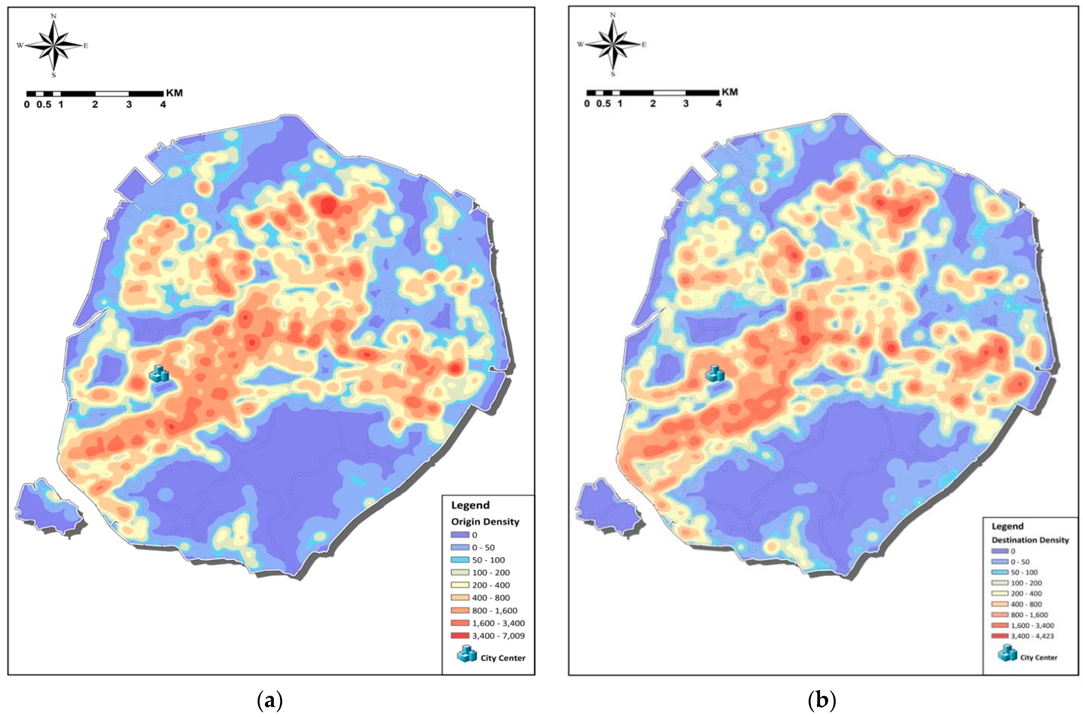
3.1. Study Area

Xiamen, located on the southeast coast of China, is a prefecture level city under the jurisdiction of Fujian Province. This paper selects Xiamen Island as the study area, which is the location of the economic, political, cultural, and financial center of Xiamen and the region with the highest level of urbanization, as shown in Figure 2. In addition, Xiamen Island concentrates many important public transportation and basic services. As of 2021, Xiamen Island has an area of 158 km² and a permanent population of about 2.1 million. According to the cycling report of major cities in China in 2017, Xiamen ranks first in terms of per capita cycling times and the level of bike-sharing use, and is rated as “the city that loves cycling most”. Therefore, choosing Xiamen Island as the study area to explore nonlinear and threshold effects of the built environment on the daily origin–destination (OD) bike-sharing ridership has full reference value and significance.

3.2. Data Sources

Bike-sharing order and GPS trajectory data. This part of the data comes from the bike-sharing trajectory data [41] released by the Xiamen government in morning peak hours, from 6:00–10:00 a.m., 21–25 December 2020. We first cleaned the data, including eliminating outliers trips such as riding position outside the study area and those with abnormally short or long riding times, and used the interpolation method to estimate missing values to ensure data consistency. Subsequently, we carried out coordinate transformation and spatial matching, and obtained all the daily origin–destination (OD) bike-sharing ridership information in the study area.

GIS layers. The study area is divided into 143 census tracts based on the administrative boundary, and the relevant road networks data are obtained through OpenStreetMap.

Built environment data. Built environment refers to the artificial space environment made for human activities, including land use, urban design, transportation infrastructure, and other factors. Accurately depicting the built environment is the key to exploring the impact of the built environment on travel behavior. The built environment is measured by the three Ds, namely, density, design, and land use diversity. Density measures include transportation density, public facilities and services density, subway density, bus density, point of interest (POI) density [42] the ratios of residential, industrial, and commercial land use, population density, and local population density. Design refers to the measurement of the characteristics of the road network in the area, measured by the road density. Land use diversity measures the mixing degree of different land uses in the region. Its measurement method is based on regional entropy and grid, and the entropy index ranges from 0 to 1, where the smaller the value, the lower the mixing degree, and 1 means that all land use types are allocated equally here [43].

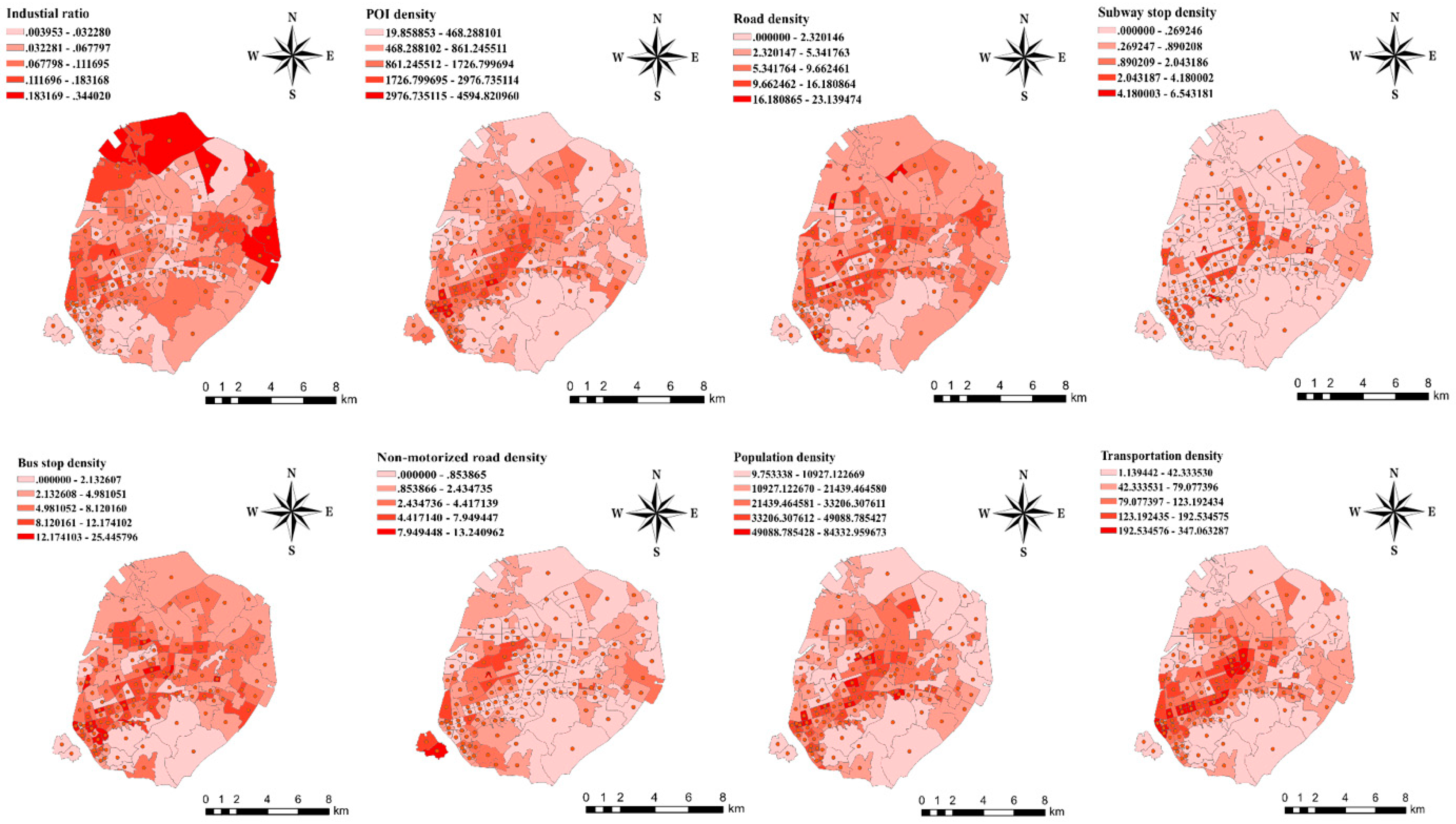
3.3. Variables Description

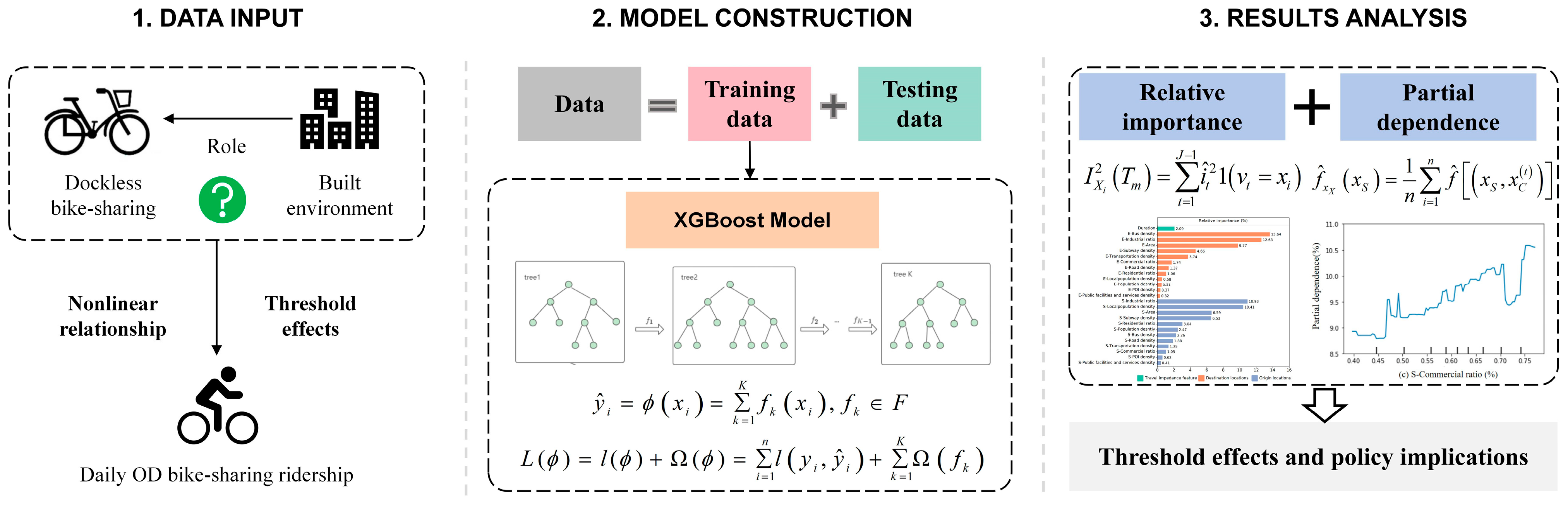
After preparing the processed basic data and determining the indicators and corresponding calculation methods, we calculated all the variables involved at a census tract level. Specifically, daily OD bike-sharing ridership is regarded as a dependent variable. Kernel density analyses of both the origins and destinations were carried out using ArcGIS Desktop 10.8 (2020) to present the spatial distribution of bike-sharing trips, as shown in Figure 3. The built environment data were regarded as explanatory variables, in which the built environment variables were further subdivided into the built environment of the origin locations and the built environment of the destination locations. In addition, the duration was selected as the travel impedance variable, which was also taken as one of the explanatory variables. Finally, all variables were statistically summarized, as described in

Table 2. Variable definitions and statistics.

Variables	Variable Description	Mean	S.D.	Min	Max
Orders
Daily OD bike-sharing ridership	Number of bike-sharing ridership from 21 to 25 December 2020	9.41	42.01	0.25	1747.75
Built environment
Population density	Population/area size (person per km2)	25,118.58	16,232.40	9.75	84,332.96
Local population density	Local population/area size (person per km2)	14,888.19	12,646.27	0	61,492.02
Transportation density	Number of transportation facilities/area size (facility per km2)	93.62	70.81	1.14	347.06
Public facilities and services density	Number of public service facilities/area size (facility per km2)	173.04	125.36	6.67	560.70
Subway density	Number of subway stations/area size (facility per km2)	0.39	1.07	0	6.54
Bus density	Number of bus stations/area size (facility per km2)	6.52	4.39	0	25.45
POI density	Number of POI/area size (facility per km2)	1097.31	861.02	19.86	4594.82
Commercial ratio	Number of commercial locations/number of POI	59.91%	12.22%	25.86%	86.94%
Residential ratio	Number of residential locations/number of POI	6.20%	2.87%	0.57%	18.84%
Industrial ratio	Number of industrial locations/number of POI	6.74%	5.90%	0.40%	34.40%
Area	Area of every tract (km2)	1.02	1.57	0.08	11.69
Road density	Length of the road/area size (km/km2)	5.92	4.58	0	23.14
Travel impedance variable
Duration	Average riding time for OD bike-sharing orders (s)	1154.35	800.01	70.00	10,069.00

below, and Figure 4 shows a visual display of the spatial distributions of some explanatory variables.

4. Methodology

4.1. Extreme Gradient Boosting—XGBoost

This study adopts a machine learning approach, the extreme gradient boosting (XGBoost) model, to investigate built environment effects on daily OD bike-sharing ridership. For classification, sorting, and regression problems, XGBoost takes into account both speed and efficiency, adopts the method of parallel tree promotion, accelerates the speed of model learning, is compatible with different platforms and language environments, and strengthens the nonlinear learning ability and scalability, so it has significant advantages of high efficiency and portability in many prediction problems and practical applications.

The core idea of XGBoost is to learn a new function every time to fit the residual of the last prediction, and to calculate the corresponding score of each node according to the characteristics of the sample [38]. The sum of all the scores is the predicted value of the sample, that is,

$${\widehat{y}}_i=\varphi \left(x_i\right)={\displaystyle {\sum }_{k=1}^K{f}_k\left(x_i\right),f_k\in F}$$

(1)

where ${\widehat{y}}_i$ is the predicted dependent variable, $x_i$ is the explanatory variable, $K$ represents the total number of samples, $f_k$ is the $kth$ tree with leaf scores, and $F$ represents all possible CARTs.

The goal is to minimize the objective function composed of loss function and regular term:

$$L\left(\varphi \right)=l\left(\varphi \right)+\Omega \left(\varphi \right)={\displaystyle \sum _{i=1}^{n}l\left(y_i,{\widehat{y}}_i\right)}+{\displaystyle \sum _{k=1}^K\Omega \left(f_k\right)}$$

(2)

where

$$\Omega \left(f\right)=\gamma T+{\displaystyle \frac{1}{2}}\lambda {\displaystyle {\sum }_{j=1}^T{\omega }_j^2}$$

(3)

where $l$ and $\Omega$ represent the loss term of measuring accuracy performance and the regular term of punishing the complexity of the model, respectively. $y_i$ is the actual dependent variable, $\gamma$ represents the complexity of each leaf, and $T$ is the number of leaves. $\lambda$ is a compromise parameter and ${\omega }_j$ means the score of the $jth$ leaf.

By solving Equations (1)–(3) with the help of Taylor expansion and other methods, the optimal weight value of the $jth$ leaf and the corresponding optimal value can be obtained as follows:

$$w_j=-{\displaystyle \frac{{\displaystyle {\sum }_{\in I_j}{g}_i}}{\left({\displaystyle {\sum }_{i\in I_j}{h}_i}+\lambda \right)}}$$

(4)

$$L^{\left(t\right)}=-{\displaystyle \frac{1}{2}}{\displaystyle \sum _{j=1}^T\frac{{\left({\displaystyle {\sum }_{\in I_j}{g}_i}\right)}^2}{{\displaystyle {\sum }_{i\in I_j}{h}_i}+\lambda }+}\gamma T$$

(5)

where

$$g_i={\partial }_{{{\widehat{y}}_i}^{(t-1)}}l\left(y_i,{{\widehat{y}}_i}^{(t-1)}\right)$$

(6)

$$h_i={{\partial }^2}_{{{\widehat{y}}_i}^{(t-1)}}l\left(y_i,{{\widehat{y}}_i}^{(t-1)}\right)$$

(7)

Since it is impossible to calculate all possible tree structures, it is necessary to rely on the greedy criterion of node recursive splitting to realize the generation of trees, and the loss reduction equation after splitting is as follows:

$$L_{split}={\displaystyle \frac{1}{2}}\left[{\displaystyle \frac{{\left({\displaystyle {\sum }_{i\in I_L}{g}_i}\right)}^2}{{\displaystyle {\sum }_{i\in I_L}{h}_i}+\lambda }}+{\displaystyle \frac{\left({\displaystyle {\sum }_{i\in I_R}{g}_i}\right)}{{\displaystyle {\sum }_{i\in I_R}{h}_i}+\lambda }}-{\displaystyle \frac{{\left({\displaystyle {\sum }_{i\in I}{g}_i}\right)}^2}{{\displaystyle {\sum }_{i\in I}{h}_i}+\lambda }}\right]-\gamma$$

(8)

where $I_L$ and $I_R$ are the instances sets of left nodes right nodes after the split, respectively, and $I=I_L\cup I_R$.

4.2. Relative Importance

In generating the decision tree, each explanatory variable has a certain probability to be selected to segment the data, and the relative importance is essentially the proportion of the number of times an explanatory variable is selected in the iterative process of generating the decision tree to the total number of times all explanatory variables are selected, and the sum of the relative importance of all explanatory variables is 100%. Relative importance is used to accurately express the contribution of an explanatory variable to the predicted dependent variable, which can be described as follows:

$$I_{X_i}^2\left(T_m\right)={\displaystyle \sum _{t=1}^{J-1}{\widehat{i}}_t^{2}1\left(v_t=x_i\right)}$$

(9)

$$I_{X_i}^2={\displaystyle \frac{1}{M}}{\displaystyle \sum _{m=1}^M{I}_{X_i}^2\left(T_m\right)}$$

(10)

where $X_i$ represents the explanatory variable, $J$ and $J-1$ represent the number of leaf nodes and non-leaf nodes of the tree, respectively, $v_t$ is a feature associated with node $t$, and the reduction in square loss after node splitting is expressed as ${\widehat{i}}_t^2$.

4.3. Partial Dependence Plots

By visualizing the relationship between dependent variables and explanatory variables, the partial dependence plots can intuitively represent the marginal effect of explanatory variables on dependent variables, and examine the influence mode of element characteristics on tag values [44]:

$${\widehat{f}}_{x_X}\left(x_S\right)=E_{x_C}\left[\widehat{f}\left(x_S,x_C\right)\right]={\displaystyle \int \widehat{f}\left(x_S,x_C\right)dP\left(x_C\right)}$$

(11)

$${\widehat{f}}_{x_X}\left(x_S\right)={\displaystyle \frac{1}{n}}{\displaystyle \sum _{i=1}^n\widehat{f}\left[\left(x_S,x_C^{\left(t\right)}\right)\right]}$$

(12)

where $x_S$ represents the variables that need to explore the nonlinear effects and $x_C$ refers to the remaining variables involved.

5. Results and Discussion

5.1. Performance of the XGBoost Model

In this paper, hyperparameter grid search is used to adjust parameters, and set the number of iterations (100, 500, 1000, 5000, 10,000), the max depth (3, 4, 5, 6, 7), and the learning rate (0.01, 0.05, 0.1). Finally, the optimal parameters to achieve the best model performance are obtained; the number of iterations, max depth, and learning rate are 5000, 5, and 0.01, respectively. In addition, pseudo-R2, mean absolute error (MAE), mean squared error (MSE), and explained variance score (EVS) for the XGBoost model are selected as the evaluation index of the model; the results are 0.7865, 6.4285, 314.0681, and 0.7867, respectively.

5.2. Relative Importance of the Explanatory Variables

Figure 5 shows the relative importance of all independent variables in predicting daily OD bike-sharing ridership and their importance rankings. The sum of the relative importance of all explanatory variables, including the built environment variables at the origin locations, the built environment variables at the destination locations, and the travel impedance variable, is 100%.

In general, the impact of the destination built environment variables on the bike-sharing ridership is slightly greater than that of the origin built environment variables, and the sum of the relative importance of the former is 50.38%, while the latter is 47.53%.

Obviously, the top six variables of relative importance are the bus density at the destination locations, the industrial ratio at the destination locations, the industrial ratio at the origin locations, the local population density at the origin locations, the area at the destination locations, and the area at the origin locations, which are 13.64%, 12.63%, 10.93%, 10.41%, 9.77%, and 6.59%, respectively. In addition, the impact of POI density and public facilities and service density on the bike-sharing ridership is relatively slight, less than 1% at both the origin and destination.

In addition, there are some variables that make a trivial contribution to the OD bike-sharing ridership, which are population density at the destination locations, local population density at the destination locations, commercial ratio at the origin locations, residential ratio at the destination locations, transportation density at the origin locations, and road density at the destination locations, with relative importances of 0.51%, 0.58%, 1.05%, 1.06%, 1.35%, and 1.37%, respectively.

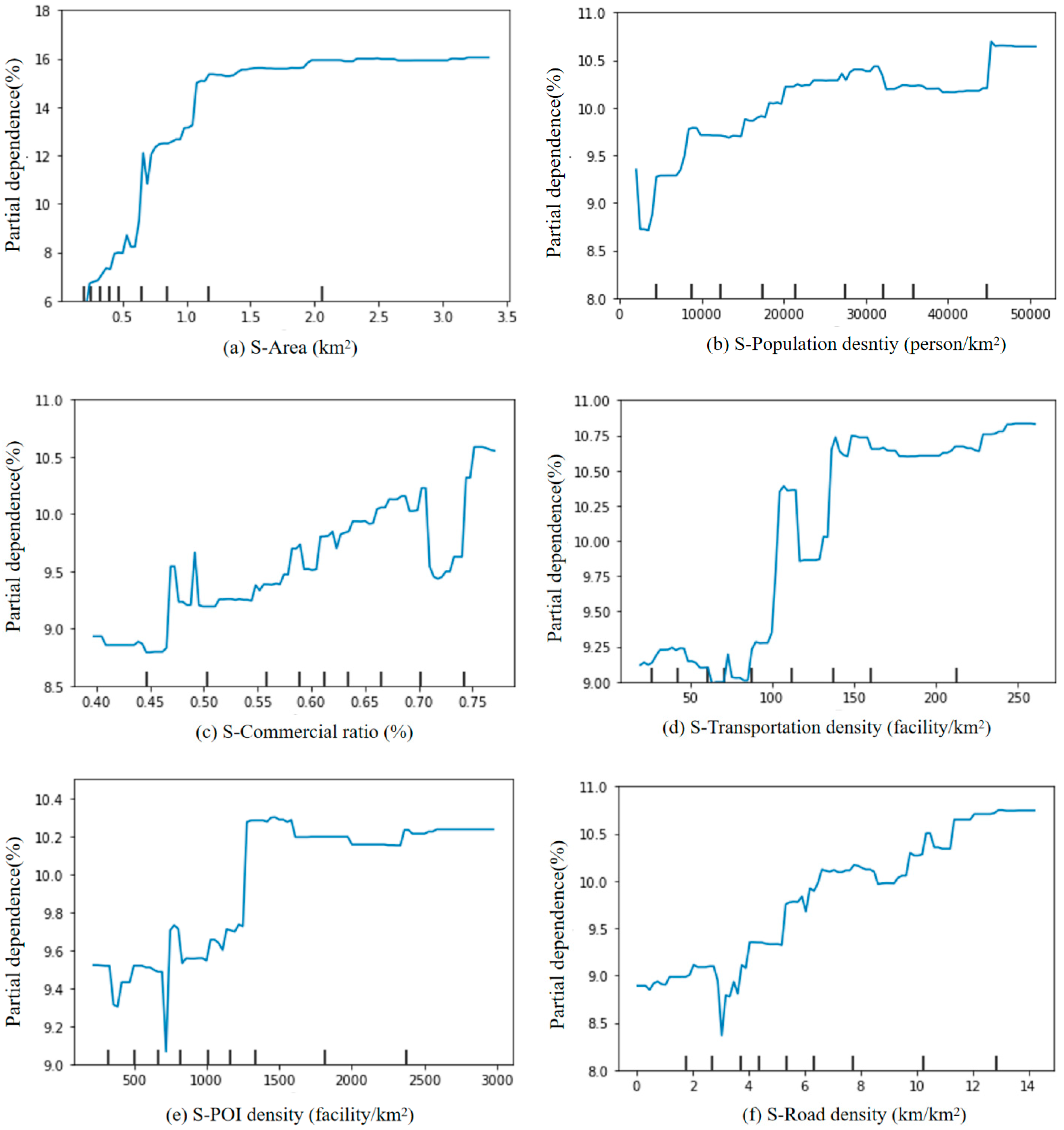
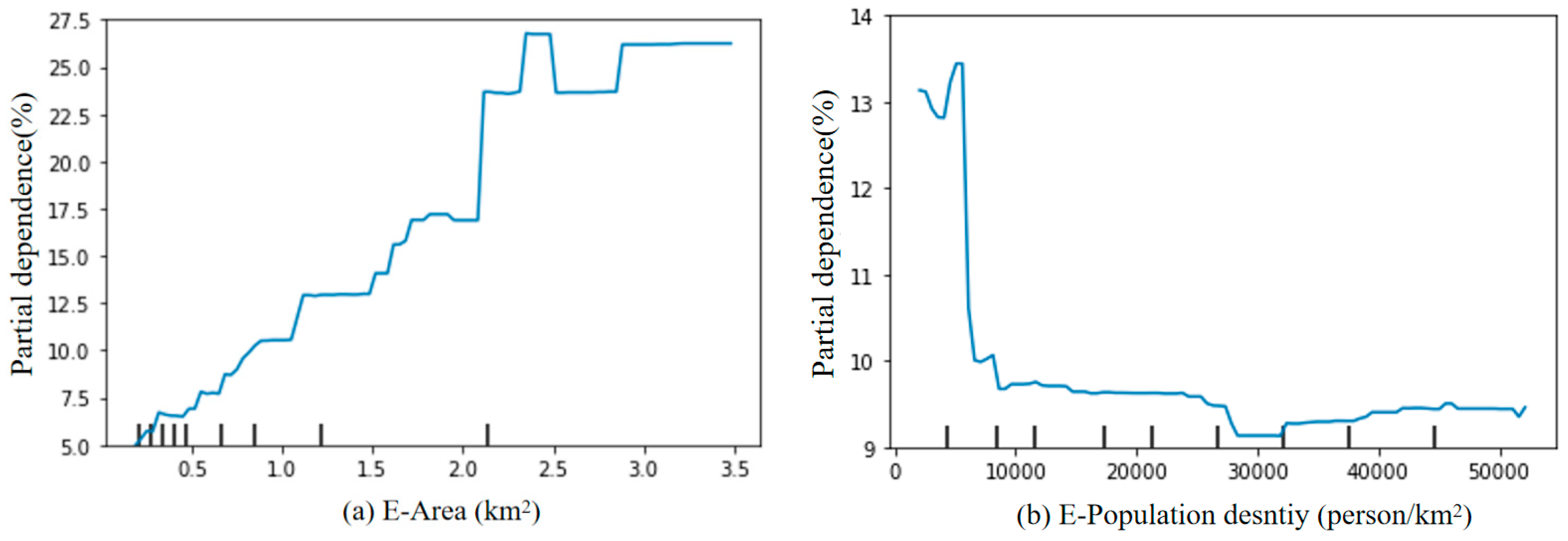
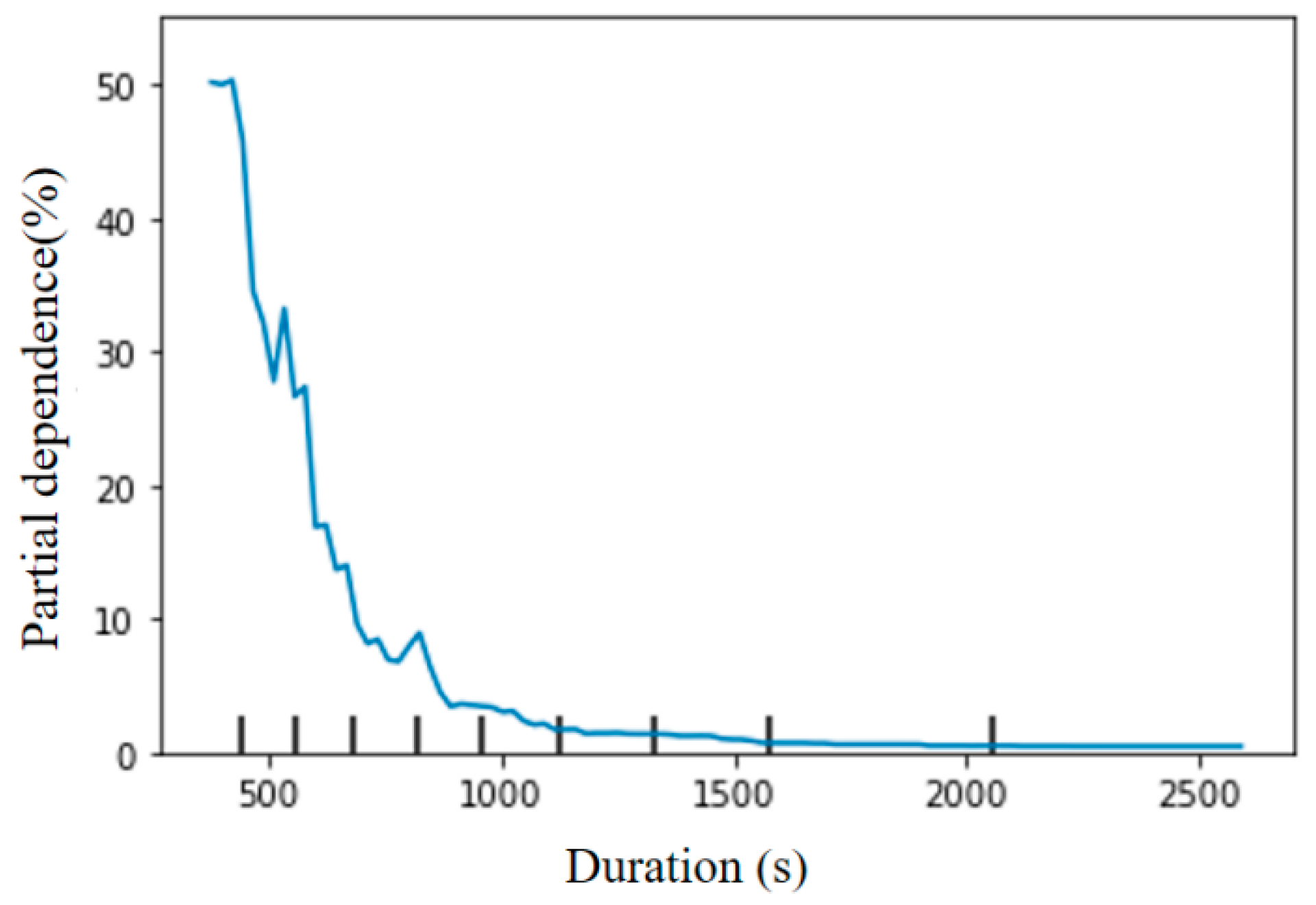
5.3. Nonlinear Associations between Key Explanatory Variables with Bike-Sharing Ridership

Figure 6 reveals the nonlinear associations between key explanatory variables at the origin locations with daily OD bike-sharing ridership. Figure 6a confirms that the area at the origin is positively correlated with the bike-sharing ridership. When the area is greater than 0.6 km², the ridership increases rapidly, and then remains at a certain level after the area is greater than 1.2 km². The area with a too-small area basically adopts walking travel. When a certain area is reached, the travel distance is too far for walking, and then people choose riding. For example, the size of a university is generally about 0.6 km² to 2 km², which is also one of the areas with the highest demand for shared bicycle riding.

Figure 6b explains that the population density at the origin has a positive impact on the bike-sharing ridership. After the population density reaches 10,000 person/km², the upward trend of the nonlinear curve becomes gentle, and the final partial dependence reaches about 10.7%. The higher the population density, the closer the area may be to the city center, the less people travel by car, and the more people choose to walk, bike, or use public transportation. In addition, the shorter the distance of travel demand, the greater the possibility of bike-sharing travel.

Figure 6c reflects that the bike-sharing ridership will be enhanced with the increase in the commercial ratio at the origin. When the commercial ratio increased from 0.45 to 0.7, the partial dependence increased from 8.8% to 10.3%, and then experienced a decline and a rapid rise. The high commercial ratio means that shopping malls, restaurants, entertainment places, etc., are relatively dense, and the travels between places are concentrated in medium- and short-distance travel, so the demand for cycling naturally increases.

Figure 6d shows the typical nonlinear relationship between transportation density at the origin and OD bike-sharing ridership, which fluctuates horizontally first, then rises sharply, then fluctuates again, and finally continues to rise and maintain at a certain level. Among them, the transportation density values corresponding to the two sudden increases are 100 facility/km² and 130 facility/km², respectively, and the density threshold is about 150 facility/km².

Figure 6e indicates that the POI density at the origin plays an active role in the bike-sharing ridership. When the POI density reached about 1250 facility/km², the ridership increased sharply, peaked at 1500 facility/km², and then the curve decreased slightly, basically maintaining the level. To a certain extent, the POI density represents the land development situation and the activity intensity in the region, and the increase in POI density may reduce the travel range of residents and increase the intensity of cycling travel.

In Figure 6f, the road density is significantly positively correlated with the bike-sharing ridership. The road density increases from 0 km/km² to 12 km/km², and the ridership increases significantly. When the road density is greater than 12 km/km², its impact on the bicycle sharing utilization rate remains almost unchanged. High road density means high accessibility, which provides convenient access to nearby areas for traffic travelers. High accessibility and convenience provide conditions for the passing and use of shared bicycles.

Figure 6g shows that although there is a certain disturbance, the subway density at the origin is basically positively associated with the bike-sharing ridership, especially in the interval with subway density of 0 facility/km² to 4 facility/km²; partial dependence rises, zigzagging from 9.3%, until it reaches the peak of 11.2%, when the subway density is about 4 facility/km², and then remains constant after a slight decrease. This shows that connecting the subway is a major function of bike-sharing.

Figure 6h displays the nonlinear effect between bus density at the origin and bike-sharing ridership, which first increases rapidly, and then peaks when the bus density reaches about 5 facility/km², and then decreases slightly and fluctuates slightly; the partial dependence is saturated at about 10.2%. In the case of this study, when the bus density is relatively high, the connection between buses and bike-sharing is strengthened, and bike-sharing is more complementary to connecting buses rather than replacing them.

To summarize the above threshold effects of the built environment at the origin, we can say that the bike-sharing ridership is higher when:

(a)

The area is greater than 1.5 km²;

(b)

The population density is greater than 10,000 person/km²;

(c)

The commercial ratio is greater than 0.6;

(d)

The transportation density is greater than 150 facility/km²;

(e)

The POI density is greater than 1500 facility/km²;

(f)

The road density is greater than 12 km/km²;

(g)

The subway density is greater than 4 facility/km²;

(h)

The bus density is greater than 4 facility/km².

Figure 7 explores the nonlinear impact of six variables at the destination on daily OD bike-sharing ridership. Figure 7a shows that the area at the destination also positively affects the bike-sharing ridership, also showing a linear positive correlation. As the area increases from 0 km² to 2 km², the partial dependence gradually increases from 5% to 17.5%. Then the curve accelerates and increases, and reaches the peak at the area of 2.5 km², about 27.5%. As the area further increases to 3 km², the curve reaches saturation and no longer fluctuates.

Figure 7b reveals that the nonlinear effect of the population density at the destination on the bike-sharing ridership is diametrically opposite to the impact of the population density at the origin.

When the population density is about 5000 person/km², the curve drops rapidly, and the partial dependence drops sharply from 13.5% to 9.5%. Later, except for insignificant fluctuations, the curve basically stays level. As mentioned earlier, the higher the population density, the closer it may be to the city center, so the demand for riding directly here will be greatly reduced.

Figure 7c indicates that the industrial ratio at the destinations actively promotes the increase in bike-sharing ridership. Before the industrial ratio reaches 0.15, the partial dependence increases with the increase in the industrial ratio, and after the industrial ratio reaches 0.15, the partial dependence reaches saturation and remains at 9.9%.

The nonlinear relationship curve in Figure 7d also shows that the transportation density at the destinations positively promotes the bike-sharing ridership, and the partial dependence gradually increases from 8% to 11.5%. The curve enters the platform period from the transportation density of 150 facility/km², then has a small increase, and finally reaches the peak at the density of about 250 facility/km² and remains stable.

Figure 7e demonstrates that the road density at the destination also significantly improves the bike-sharing ridership. When the road density increases from 4 km/km² to 7 km/km², the curve continues to rise, and the partial dependence increases from 9% to 10.3%. After the road density reaches 7 km/km², the curve will no longer continue to rise with the increase in density. Similar to Figure 7f above, the higher the road density, the more sufficient the road conditions for riding.

Figure 7f also visually shows the positive correlation between bus density at the destination and bike-sharing ridership. Obviously, when the bus density is 6 facility/km², the partial dependence increases rapidly and finally stabilizes at 11%. Compared with the effect of the bus density at the origin on the bike-sharing ridership, both of them promote the ridership, but one switches to bike-sharing to the destination after the bus trip, and the other rides to the bus station.

To summarize the above threshold effects of the built environment at the destination, we can say that the bike-sharing ridership is higher when:

(a)

The area is greater than 2 km²;

(b)

The population density is less than 10,000 person/km²;

(c)

The industrial rate is greater than 0.15;

(d)

The transportation density is greater than 150 facility/km²;

(e)

The road density is greater than 4 km/km²;

(f)

The bus density is greater than 6 facility/km².

In terms of travel impedance variable, Figure 8 clearly depicts the obvious negative correlation between duration and bike-sharing ridership, that is, ridership continues to decrease with the growth of duration. When the duration is more than 15 min, people are almost unwilling to choose bike-sharing for travel, which is in line with the purpose of bike-sharing for short- and medium-distance travel.

5.4. Multipredictor Partial Dependence Plot

Figure 9 indicates the superposition effect of bus density at the destination and subway density at the destination on daily OD bike-sharing ridership. It can be seen from the three-dimensional partial dependence plot that the partial dependence reaches the lowest value when the bus density is less than 4 facility/km² and the subway density is less than 1 facility/km², and reaches the maximum value when the bus density is between 4 facility/km² and 8 facility/km² and the subway density is between 4 facility/km² and 6 facility/km².

6. Conclusions and Implications

To achieve refined management for bike-sharing systems, this study applied XGBoost, a machine learning algorithm, to analyze the nonlinear and threshold effects between the built environment and the OD bike-sharing ridership from the street community level, using empirical data from Xiamen Island in China. First, we calculated the relative importance, and statistically described the impact and difference of each explanatory variable on the prediction of the OD bike-sharing ridership. Subsequently, we further extracted and drew the partial dependence plot to capture the nonlinear effect of built environment on OD bike-sharing ridership, and explored the quantitative relationship between each important influence factor and OD bike-sharing ridership.

The research results not only enable relevant managers and planning decision-makers to have a deeper understanding of the role of built environment in the dockless bike-sharing travel mode, but they also provide certain insights and guidance for urban land use renewal, public transport station development and construction, and dockless bike-sharing operation and management.

The relative importance results indicate that the built environment at the origin and destination has great effects on the daily OD bike-sharing ridership, and the overall relative importance is relatively close, at 47.53% and 50.38%, respectively. From the point of origin locations, the industrial ratio, local population density, area, and subway density have a significant impact on predicting OD bike-sharing ridership, with a total relative importance of 34.46%. From the perspective of destination locations, the variables with higher relative importance are bus density, industrial ratio, area, and subway density, which are 13.64%, 12.63%, 9.77%, and 4.66%, respectively. In general, industrial ratio, area, bus, and subway density are of great importance to predict OD bike-sharing ridership at both the origin and destination.

Effective ranges and the thresholds of the built environment factors are identified via partial dependence plots to provide the policy implications for promoting bike-sharing systems. It was found that when the transportation density at the origin or at the destination is greater than 150 facility/km², the bike-sharing ridership is higher, which reveals that it is necessary to continue to scientifically and reasonably improve transportation facilities and help the development of urban public transport on the basis of meeting the development goals of the Chinese public transport system. Most importantly, we focused on the positive impact of the bus density and subway density variables on OD bike-sharing ridership, which, to a certain extent, explains that at the planning and bicycle release level, we should advocate the seamless connection design of bus stations, subway stations, and bike-sharing release locations, so as to facilitate the connection of “the first kilometer” and “the last kilometer” of public transport and expand the coverage of urban public transport.

The findings could provide policy implications for target audiences of different groups. For urban planners, when actively planning and intervening in urban space from different dimensions such as density, diversity, and design, the adaptability of bike-sharing travel activities to the built environment can be appropriately taken into account to improve the bike-sharing riding space. For bike-sharing operating companies, the configuration can be optimized to achieve more scientific bike-sharing delivery, provide sufficient bike-sharing services in areas with high bike demand, and appropriately reduce the shared bike capacity in areas with low bike demand, so as to improve the travel efficiency of bike-sharing and improve the turnover rate.

Of course, there are still some deficiencies in this paper, and the following aspects could be further explored in the future. In this paper, our research case is a typical bay city, and it is necessary to select more plain cities with different geographical and geometric characteristics to analyze and compare the heterogeneity of the nonlinear relationship between the built environment and bike-sharing ridership. Furthermore, different methods could be compared, such as multilayer neurocontrol of high-order uncertain nonlinear systems and integral robust schemes for mismatched uncertain nonlinear systems. The impact and mechanisms of the built environment on the competition and cooperation relationship between bike-sharing and other traffic modes could be further research directions.

References

1. Jiang, H.; Song, S.; Zou, X.; Lu, L. How Dockless Bike Sharing Changes Lives: An Analysis of Chinese Cities. 2020. Available online: https://www.wri.org/research/how-dockless-bike-sharing-changes-lives-analysis-chinese-cities (accessed on 10 May 2024).
2. Gonzalez, F.; Melo-Riquelme, C.; Grange, L.D. A combined destination and route choice model for a bicycle sharing system. Transportation 2016, 43, 407–423. [Google Scholar] [CrossRef]
3. Si, H.; Shi, J.; Wu, G.; Chen, J.; Zhao, X. Mapping the Bike Sharing Research Published from 2010 to 2018: A Scientometric Review. J. Clean. Prod. 2019, 213, 415–427. [Google Scholar] [CrossRef]
4. Guo, Y.; Yang, L.; Chen, Y. Bike Share Usage and the Built Environment: A Review. Front. Public Health 2022, 10, 848169. [Google Scholar] [CrossRef] [PubMed]
5. Babagoli, M.A.; Kaufman, T.K.; Noyes, P.; Sheffield, P.E. Exploring the Health and Spatial Equity Implications of the New York City Bike Share System. J. Transp. Health 2019, 13, 200–209. [Google Scholar] [CrossRef]
6. Bullock, C.; Brereton, F.; Bailey, S. The Economic Contribution of Public Bike-Share to the Sustainability and Efficient Functioning of Cities. Sustain. Cities Soc. 2017, 28, 76–87. Available online: https://www.sciencedirect.com/science/article/abs/pii/S2210670716303080 (accessed on 17 August 2024). [CrossRef]
7. Kim, M.; Cho, G.-H. Analysis on Bike-Share Ridership for Origin-Destination Pairs: Effects of Public Transit Route Characteristics and Land-Use Patterns. J. Transp. Geogr. 2021, 93, 103047. [Google Scholar] [CrossRef]
8. Lahoorpoor, B.; Faroqi, H.; Sadeghi-Niaraki, A.; Choi, S.M. Spatial Cluster-Based Model for Static Rebalancing Bike Sharing Problem. Sustainability 2019, 11, 3205. [Google Scholar] [CrossRef]
9. Ma, X.; Ji, Y.; Yuan, Y.; Van Oort, N.; Jin, Y.; Hoogendoorn, S. A Comparison in Travel Patterns and Determinants of User Demand between Docked and Dockless Bike-Sharing Systems Using Multi-Sourced Data. Transp. Res. Part A Policy Pract. 2020, 139, 148–173. [Google Scholar] [CrossRef]
10. Xue, X.; Wang, Z.; Liu, X.; Zhou, Z.; Song, R. A Choice Behavior Model of Bike-Sharing Based on User Perception, Psychological Expectations, and Loyalty. J. Adv. Transp. 2022, 2022, 6695977. [Google Scholar] [CrossRef]
11. Sun, C.; Lu, J. Modeling Spatial Riding Characteristics of Bike-Sharing Users Using Hotspot Areas-Based Association Rule Mining. J. Adv. Transp. 2022, 2022, 5705080. [Google Scholar] [CrossRef]
12. Ding, C.; Cao, X.; Liu, C. How Does the Station-Area Built Environment Influence Metrorail Ridership? Using Gradient Boosting Decision Trees to Identify Non-Linear Thresholds. J. Transp. Geogr. 2019, 77, 70–78. [Google Scholar] [CrossRef]
13. Shao, Q.; Zhang, W.; Cao, X.; Yang, J.; Yin, J. Threshold and Moderating Effects of Land Use on Metro Ridership in Shenzhen: Implications for TOD Planning. J. Transp. Geogr. 2020, 89, 102878. [Google Scholar] [CrossRef]
14. Tao, T.; Wang, J.; Cao, X. Exploring the Non-Linear Associations between Spatial Attributes and Walking Distance to Transit. J. Transp. Geogr. 2020, 82, 102560. [Google Scholar] [CrossRef]
15. Yu, H.; Peng, Z.-R. Exploring the Spatial Variation of Ridesourcing Demand and Its Relationship to Built Environment and Socioeconomic Factors with the Geographically Weighted Poisson Regression. J. Transp. Geogr. 2019, 75, 147–163. [Google Scholar] [CrossRef]
16. Tu, M.; Li, W.; Orfila, O.; Li, Y.; Gruyer, D. Exploring Nonlinear Effects of the Built Environment on Ridesplitting: Evidence from Chengdu. Transp. Res. Part D Transp. Environ. 2021, 93, 102776. [Google Scholar] [CrossRef]
17. Zhang, W.; Zhao, Y.; Cao, X.; Lu, D.; Chai, Y. Nonlinear Effect of Accessibility on Car Ownership in Beijing: Pedestrian-Scale Neighborhood Planning. Transp. Res. Part D Transp. Environ. 2020, 86, 102445. [Google Scholar] [CrossRef]
18. Bi, H.; Li, A.; Hua, M.; Zhu, H.; Ye, Z. Examining the Varying Influences of Built Environment on Bike-Sharing Commuting: Empirical Evidence from Shanghai. Transp. Policy 2022, 129, 51–65. [Google Scholar] [CrossRef]
19. Zhu, L.; Ali, M.; Macioszek, E.; Aghaabbasi, M.; Jan, A. Approaching sustainable bike-sharing development: A systematic review of the influence of built environment features on bike-sharing ridership. Sustainability 2022, 10, 5795. [Google Scholar] [CrossRef]
20. Sun, Y.; Mobasheri, A.; Hu, X.; Wang, W. Investigating impacts of environmental factors on the cycling behavior of bicycle-sharing users. Sustainability 2017, 9, 1060. [Google Scholar] [CrossRef]
21. El-Assi, W.; Mahmoud, M.S.; Habib, K.N. Effects of built environment and weather on bike sharing demand: A station level analysis of commercial bike sharing in Toronto. Transportation 2017, 44, 589–613. [Google Scholar] [CrossRef]
22. Shen, Y.; Zhang, X.; Zhao, J. Understanding the usage of dockless bike sharing in Singapore. Int. J. Sustain. Transp. 2018, 12, 686. [Google Scholar] [CrossRef]
23. Zhao, D.; Ong, G.P.; Wang, W.; Hu, X. Effect of built environment on shared bicycle reallocation: A case study on Nanjing, China. Transp. Res. Part A Policy Pract. 2019, 128, 73–88. [Google Scholar] [CrossRef]
24. Luan, S.; Li, M.; Li, X.; Ma, X. Effects of Built Environment on Bicycle Wrong Way Riding Behavior: A Data-Driven Approach. Accid. Anal. Prev. 2020, 144, 105613. [Google Scholar] [CrossRef]
25. Chen, E.; Ye, Z. Identifying the Nonlinear Relationship between Free-Floating Bike Sharing Usage and Built Environment. J. Clean. Prod. 2021, 280, 124281. [Google Scholar] [CrossRef]
26. Li, Z.; Shang, Y.; Zhao, G.; Yang, M. Exploring the Multiscale Relationship between the Built Environment and the Metro-Oriented Dockless Bike-Sharing Usage. Int. J. Environ. Res. Public Health 2022, 19, 2323. [Google Scholar] [CrossRef]
27. Alemi, F.; Circella, G.; Handy, S.; Mokhtarian, P. What Influences Travelers to Use Uber? Exploring the Factors Affecting the Adoption of on-Demand Ride Services in California. Travel Behav. Soc. 2018, 13, 88–104. [Google Scholar] [CrossRef]
28. Durning, M.; Townsend, C. Direct ridership model of rail rapid transit systems in Canada. Transp. Res. Rec. 2015, 2537, 96–102. [Google Scholar] [CrossRef]
29. Özbil Torun, A.; Göçer, K.; Yeşiltepe, D.; Argın, G. Understanding the Role of Urban Form in Explaining Transportation and Recreational Walking among Children in a Logistic GWR Model: A Spatial Analysis in Istanbul, Turkey. J. Transp. Geogr. 2020, 82, 102617. [Google Scholar] [CrossRef]
30. Lu, Y.; Sun, G.; Sarkar, C.; Gou, Z.; Xiao, Y. Commuting Mode Choice in a High-Density City: Do Land-Use Density and Diversity Matter in Hong Kong? Int. J. Environ. Res. Public Health 2018, 15, 920. [Google Scholar] [CrossRef]
31. Wang, D.G.; Cao, X.Y. Impacts of the built environment on activity-travel behavior: Are there differences between public and private housing residents in Hong Kong? Transp. Res. Part A Policy Pract. 2017, 103, 25–35. [Google Scholar] [CrossRef]
32. Li, T.; Jing, P.; Li, L.; Sun, D.; Yan, W. Revealing the Varying Impact of Urban Built Environment on Online Car-Hailing Travel in Spatio-Temporal Dimension: An Exploratory Analysis in Chengdu, China. Sustainability 2019, 11, 1336. [Google Scholar] [CrossRef]
33. Hagenauer, J.; Helbich, M. A comparative study of machine learning classifiers for modeling travel mode choice. Expert Syst. Appl. 2017, 78, 273–282. [Google Scholar] [CrossRef]
34. Breiman, L. Random Forests. Mach. Learn. 2001, 45, 5–32. [Google Scholar] [CrossRef]
35. Cortes, C.; Vapnik, V. Support-Vector Networks. Mach. Learn. 1995, 20, 273–297. [Google Scholar] [CrossRef]
36. Friedman, J.H. Greedy function approximation: A gradient boosting machine. Ann. Stat. 2001, 29, 1189–1232. [Google Scholar] [CrossRef]
37. Zhuang, C.; Li, S.; Tan, Z.; Gao, F.; Wu, Z. Nonlinear and Threshold Effects of Traffic Condition and Built Environment on Dockless Bike Sharing at Street Level. J. Transp. Geogr. 2022, 102, 103375. [Google Scholar] [CrossRef]
38. Chen, T.; Guestrin, C. XGBoost: A Scalable Tree Boosting System. In Proceedings of the 22nd ACM SIGKDD International Conference on Knowledge Discovery and Data Mining (KDD), San Francisco, CA, USA, 13 August 2016. [Google Scholar]
39. Luo, Y.; Liu, Y.; Tong, Z.; Wang, N.; Rao, L. Capturing gender-age thresholds disparities in built environment factors affecting injurious traffic crashes. Travel Behav. Soc. 2023, 30, 21–37. [Google Scholar]
40. Yi, Z.; Liu, X.C.; Markovic, N.; Phillips, J. Inferencing hourly traffic volume using data-driven machine learning and graph theory. Comput. Environ. Urban Syst. 2021, 85, 101548. [Google Scholar] [CrossRef]
41. Digital China Innovation Contest, DCIC. Fu Zhou, China. 2021. Available online: https://data.xm.gov.cn/contest-series/digit-china-2021/index.html#/3/competition_data (accessed on 10 May 2024).
42. Gaode Map. Gaode API. 2021. Available online: https://lbs.amap.com/api/webservice/guide/api/search (accessed on 10 May 2024).
43. Cervero, R.; Kockelman, K. Travel Demand and the 3Ds: Density, Diversity, and Design. Transp. Res. Part D Transp. Environ. 1997, 2, 199–219. [Google Scholar] [CrossRef]
44. Hastie, T.; Tibshirani, R.; Friedman, J. The Elements of Statistical Learning: Data Mining, Inference, and Prediction; Springer Science & Business Media: Berlin/Heidelberg, Germany, 2009. [Google Scholar]
Figure 1. Schematic diagram of the research framework.
Sustainability 16 07690 g001
Figure 2. Study area.
Sustainability 16 07690 g002
Figure 3. Spatial distributions of daily bike-sharing trips. (a) Density analysis of bike-sharing trip origins. (b) Density analysis of bike-sharing trip destinations.
Sustainability 16 07690 g003
Figure 4. Distributions of some explanatory variables.
Sustainability 16 07690 g004
Figure 5. The importance ranking of all the explanatory variables, Note: “S-” represents factors at the origin locations, and “E-” represents factors at the destination locations.
Sustainability 16 07690 g005
Figure 6. The effects of the key variables at the origin on the daily OD bike-sharing ridership.
Sustainability 16 07690 g006aSustainability 16 07690 g006b
Figure 7. The effects of the key variables at the destination on the daily OD bike-sharing ridership.
Sustainability 16 07690 g007aSustainability 16 07690 g007b
Figure 8. The effects of the duration on the daily OD bike-sharing ridership.
Sustainability 16 07690 g008
Figure 9. The combined effects of E-subway density and E-bus density on the daily OD bike-sharing ridership.
Sustainability 16 07690 g009