Integrating the Energy Performance Gap into Life Cycle Assessments of Building Renovations

Abstract

The environmental impact of building energy renovation is commonly evaluated through life cycle assessment (LCA). However, existing LCA studies often overlook the energy performance gap—a substantial disparity between calculated and actual energy use—when estimating operational energy use before and after renovation. This paper examines the influence of the energy performance gap on the comparative LCA between unrenovated and renovated buildings. First, a statistical correction model, based on a recent large-scale Flemish study, is developed to correct regulatory calculated energy use for space heating and domestic hot water in a pragmatic way. Subsequently, the model is applied to four single-family dwellings with different energy characteristics that underwent renovation in accordance with Flemish energy regulations. The results show that the anticipated environmental savings over a 60-year study period decrease significantly when the correction model is applied, reducing the estimated savings of 49–80% to 21–49%. Moreover, environmental payback times increase from 2.9–9.1 years to 10.4–22.5 years. Notably, neglecting the energy performance gap in LCAs leads to systematic underestimations of the material use significance. This research underscores the importance of integrating the energy performance gap into LCAs to obtain more accurate estimations of the environmental benefits of energy renovations.

1. Introduction

The European Union (EU) aims to reduce greenhouse gas (GHG) emissions by at least 55% by 2030 and 80% by 2050 compared to the 1990s level [1,2]. Given that 85–95% of the existing EU buildings will still be in use by 2050, there is an urgent need for energy renovations [3]. Currently, only a mere 1% of the EU building stock undergoes some degree of energy renovation annually. Moreover, the annual rate of deep energy renovations, which involve reducing energy use by at least 60%, is only 0.2% [3]. This rate is far below the proposed 2% target in the Renovation Wave [3] as well as the necessary 3% rate for a full renovation of the EU building stock by 2050 [4]. Renovating all EU residential buildings could potentially reduce final energy use for space heating by 44% [5], significantly contributing to the EU’s GHG reduction goals. However, this process requires significant amounts of building materials and causes high waste streams. As a result, adopting a life cycle approach becomes crucial to ensure a sustainable transition.

1.1. Environmental Impact of Energy Renovations

Life cycle assessment (LCA) is commonly applied to evaluate the environmental impact of building energy renovations, encompassing both operational energy use and embodied impact. Multiple researchers [6,7,8,9,10,11,12,13,14,15,16,17,18,19,20,21,22,23,24,25] compared different renovation measures—from enhancing the building envelope to incorporating renewable energy sources—and assessed these measures against a reference scenario, where the existing poorly or non-insulated building is preserved without any energy improvements.

Table 1. Summary of the literature on the environmental impact of renovation measures.

Reference	Country	Case	RSP	Measures	Environmental Savings	Payback Time in Years
Dominguez et al. [6]	DE	SF	25	BE, HS, PV, SC	GWP: 36–83%	-
Passer et al. [7]	AT	MF	60	BE, PV, SC	GWP: 67–77% CED: 67–98%	CED: 2–10
Conci et al. [8]	DE	MF	30	BE, HS, PV, SC	GWP: 58–75%	-
Chandrasekaran et al. [9]	LT	MF	40	BE, HS, SC	GWP: 12–48%	-
Oliveira Fernandes et al. [10]	NL	SF, MF	30	BE, HS, PV	SS: 13–62%	-
Vavanou et al. [11]	UK	SF	60	BE, HS, HR, PV, SC	GWP: 30–77%	-
González-Prieto et al. [12]	ES	NR	100	BE, HS, PV	GWP: 25–59% CED: 27–69%	-
Apostolopoulos et al. [13]	GR	MF	25	BE, HS, HR, PV, SC	GWP: 95% PE: 91%	GWP: 2 PE: 3
Struhala and Ostrý [14]	CZ	SF	60	BE, HS, SC	SS: 58–90%	-
Rabani et al. [15]	NO	NR	60	BE, HS, PV	GWP: 48–52%	GWP: 3.9–5.1
Khadra et al. [16]	SE	MF	50	BE, HS, HR, PV	-	GWP: 7–18
Arbulu et al. [17]	ES	SF, MF	50	BE, HS, PV	GWP: 3–91%	-
Rasmussen et al. [18]	DK	MF	60	BE, HS, PV	-	GWP: 13 PE: 18 Others: 1–4
Shirazi and Ashuri [19]	US	SF	-	BE, HS	-	PE: 1.4–5.8
Dodoo et al. [20]	SE	MF	50	BE, HR	PE: 6–32%	-
Lasvaux et al. [21]	CH	MF	60	BE, HS, HR	GWP: 76% CED: 71%	-
Ramírez-Villegas et al. [22]	SE	MF	50	BE, HR	GWP: 10–19% Others: 4–17%	-
Asdrubali et al. [23]	IT	NR	50	BE, HS	-	GWP: 3.2–6.5 PE: 2.9–7.0
Zhang et al. [24]	ES, NL, SE	MF	100	BE	-	GWP: 8.6–23.3 CED: 17.6–20.5
Wrålsen et al. [25]	NO	MF	30	BE, HS, HR	GWP: 93–95% Others: 56–96%	GWP: 1.1 CED: 2.1

Country—DE = Germany, AT = Austria, LT = Lithuania, NL = Netherlands, UK = United Kingdom, ES = Spain, GR = Greece, CZ = Czech Republic, NO = Norway, SE = Sweden, DK = Denmark, US = United States, CH = Switzerland, IT = Italy; Case—SF = single-family, MF = multi-family, NR = non-residential; RSP = Reference study period; Measures—BE = building envelope, HS = heating system, HR = ventilation with heat recovery, PV = photovoltaic, SC = solar collector; Indicators—GWP = global warming potential, CED = cumulative energy demand, PE = primary energy, SS = single score.

gives an overview of LCA studies assessing the environmental savings potential of renovating residential and non-residential buildings.

Across the examined studies, it is consistently found that energy renovation results in a reduction of the overall environmental impact compared to unrenovated buildings. The extent of these environmental savings varies from 3% to 98%. This significant variation stems from differences in the initial condition of the building, reference study period, impact indicators, specific renovation measures, etc. Nevertheless, all studies concluded that the operational energy savings due to renovation compensated for the material use of renovation (i.e., embodied impact). Within this context, several studies examined the time required for the embodied impact to be recovered through the annual operational energy savings, commonly referred to as the environmental, carbon, or energy payback time. The findings reveal a range between 1.0 and 23.3 years, a period notably short in comparison to the total service life of buildings.

The savings potential and payback times are closely linked to the difference in operational energy use between renovated and existing buildings, as operational energy use significantly contributes to the environmental impact. In the research of Lasvaux et al. [21], for example, operational energy use contributed approximately 80% of the global warming potential and cumulative energy demand of the renovated building. Similarly, Vavanou et al. [11] addressed contributions of 84–99% in life cycle CO₂ emissions.

1.2. Energy Performance Gap

LCA studies of renovation projects commonly employ theoretical models to estimate operational energy use before and after renovation. This varies between (1) simplified models such as the heating degree day method [10,26,27], (2) regulatory calculation methods used for energy performance rating and certification [7,9,14,28,29], and (3) more advanced dynamic building simulations [6,13,15,17,22,24]. However, multiple studies have shown that energy renovations often yield smaller energy savings than initially estimated [30,31,32,33,34,35]. This phenomenon is known as the ‘energy saving gap’, which represents the difference between calculated and actual energy savings. Cozza et al. [35] reported a median energy savings gap of 37% for a sample of 1172 retrofitted Swiss buildings. Additionally, van den Brom et al. [31] found that of the nearly 90,000 Dutch renovated dwellings, 57% had lower energy savings than expected and noted that the gap tended to be larger when the energy performance of the unrenovated building was worse.

The energy savings gap stems from the difference between calculated and real energy use, referred to as the ‘energy performance gap’ (EPG). Several studies from various countries have investigated the EPG [35,36,37,38,39,40]. These studies consistently found that actual energy use in old, non-insulated buildings was significantly lower than calculated energy use. As buildings improve in energy performance, the average deviation between actual and calculated values decreased. In some instances, the EPG even shifted further towards an underestimation of the actual energy use in highly efficient buildings [36,40]. In a literature review of 144 EPG studies, Mahdavi et al. [41] reported a mean EPG of about 30% in residential buildings, with a significant variability spanning from an underestimation of the actual energy use by 25% to an overestimation by 96%. Similarly, Zheng et al. [42] found in their literature review that the EPG ratios (i.e., ratio of actual over predicted energy use) ranged from 0.5 to 2.5 for residential buildings. Bai et al. [43] concluded from 76 low-energy building case studies that actual energy use was 86% lower to 483% higher than predicted, with an average relative difference of 58%.

Discrepancies between calculated and actual energy use stem from a variety of factors, making it challenging to accurately determine energy savings [41,44,45,46,47]. There are physical modeling errors that arise from inadequate design, performance, or execution quality of building envelopes [47,48,49,50] and technical installations [49,51]. Eon et al. [52] underscored that discrepancies between as-designed and as-built performance may occur during construction and commissioning stages due to a lack of knowledge, skills, and communication among stakeholders. In addition, simplifications, assumptions, and conservative values in energy models add to the EPG [44,47]. On the other hand, occupant behavior plays a crucial role. Variations in heating, ventilation, and domestic water use behavior can considerably affect energy use [47,53]. Socio-economic factors and household demographics contribute to behavioral variation, with parameters such as income, size, and energy prices influencing occupant behavior [37,46,54]. In the context of energy renovation, the literature references two phenomena to explain part of the EPG: rebound [55,56,57] and prebound effect [40,57]. Whereas the first refers to part of the energy savings being offset by increased energy use, the latter describes lower energy uses than predicted in unrenovated dwellings. Both phenomena are frequently linked to occupant behavior.

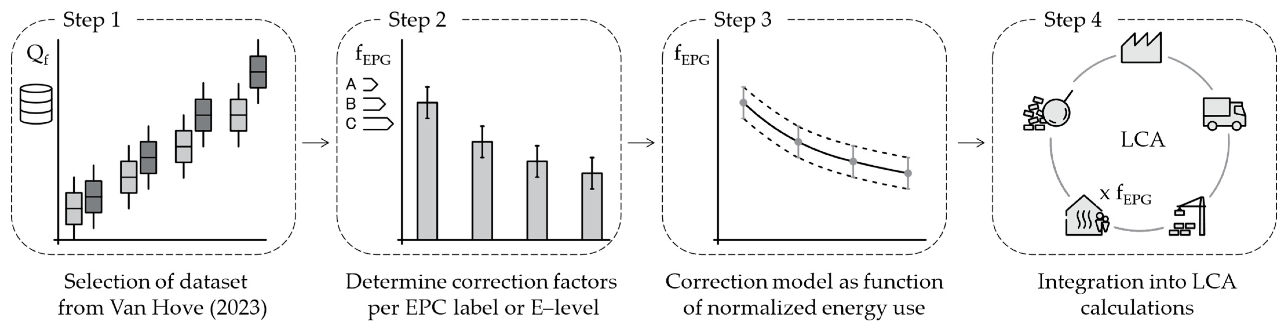
1.3. Research Goal, Scope, and Steps

The discrepancy between calculated and real energy use could have a potentially significant influence on the environmental savings potential and payback times of energy renovation, as operational energy use represents a dominant share of the environmental impact. The substantial figures reported in literature regarding the EPG emphasize the importance of addressing this aspect when conducting an LCA of energy renovations. However, current LCA research on the environmental savings potential and payback times of renovation measures generally does not consider the EPG. Consequently, the primary aim of this paper is to investigate how to incorporate the EPG into LCA calculations and to assess the influence of the EPG on the comparative LCA between unrenovated and renovated dwellings in terms of environmental savings potential and payback times.

Given the extensive data required for conducting an LCA and the multifaceted nature of factors contributing to the EPG, this study aims to develop a pragmatic correction model to adjust calculated operational energy use in LCAs. This model prioritizes simplicity and flexibility over the complexities of correcting physical building modeling. Attempting to incorporate individual causes would exceed the scope of this paper, which is to address the importance of potential discrepancies between calculated and actual energy use on the environmental savings potential and payback time of energy renovations. Notably, no studies have been found that specifically integrate the EPG into LCA calculations.

First, existing models in the literature that aim to correct calculated energy use are reviewed. Subsequently, a correction model is developed, drawing inspiration from the methods underlying these existing models. Due to substantial variation in the EPG among countries, influenced by regional and national disparities (e.g., climate conditions, construction methods, and regulatory calculation methods) [38,58], this research aims to provide an applicable model for LCAs in the Belgian context. Therefore, recent insights from a large-scale Flemish study by Van Hove et al. [38,59] addressing the EPG of single-family dwellings were employed to develop a statistical model tailored to the needs of this study. An average correction based on large-scale statistical data was found most appropriate for the analysis, as the research focuses on a synthetic sample of representative dwellings rather than a specific real-world renovation project. Moreover, the focus of this paper is on single-family dwellings, which aligns with the scope of Van Hove et al. [38,59] and is substantiated by the significant prevalence of single-family dwellings in the Belgian building stock, comprising 78% of all residential and non-residential buildings [60].

Next, the developed model is applied to four representative Flemish single-family dwellings with identical geometry but different construction years, each possessing varying initial energetic characteristics. To standardize their energy performance post-renovation, all buildings were renovated in compliance with the Flemish Energy Performance of Buildings Directive (EPBD) regulations. The environmental impact of both the unrenovated and renovated dwellings is calculated over a 60-year study period. Finally, the life cycle environmental impact, savings potential, and payback time, both without and with consideration of the EPG, are evaluated and compared to highlight the significance of incorporating the EPG in LCA applications for energy renovations.

2. Existing Models to Correct Calculated Energy Use

As mentioned, there is a consistent pattern in the EPG where actual energy use tends to be lower than the calculated values. The better the energy performance, the narrower the gap between the two. In some instances, the trend even reverses. Several researchers have explored correlations between calculated and real energy uses, leading to specific models aimed at correcting calculated energy use in a pragmatic way. An overview of such correction models is provided by Sunikka-Blank and Galvin [40].

Tigchelaar et al. [61] defined the ratio between real and calculated energy use for space heating as a ‘heating factor’, similar to the ‘energy intensity factor’ used by Cayre et al. [62]. A heating factor of one signifies equality between calculated and actual energy use, whereas a value below one indicates lower actual energy uses than expected. Their study, based on a sample of 4700 Dutch residential buildings, derived average factors in relation to Energy Performance Certificate (EPC) labels. These factors consistently fell below one, indicating a systematic overestimation of real energy use. The factors ranged from 0.88 for EPC-label A to 0.53 for EPC-label G, with a significant variability in these average factors, from 0.25 to 1.75. Analogously, Laurent et al. [58] documented correction factors as a function of EPC labels, ascertained through research conducted in both French and English contexts. For the French dwellings, factors of 1.7 (label B) to 0.4 (label G) were identified, whereas the English cases showed factors of 0.97 (label C) to 0.58 (label G) (note that each European country can determine its own classification system, which ensures that the definition of EPC labels varies significantly across countries [59,63]).

Furthermore, Loga et al. [39] formulated a different type of correction model based on a dataset of 1702 German buildings. Specifically, a correlation was defined by depicting average values of the ratio between measured and calculated energy use against normalized calculated energy use per floor area:

$${\mathrm{f}}_{\mathrm{corr}}=-0.2+1.3 / (1+{\mathrm{Q}}_{\mathrm{h},\mathrm{calc}} / 500)$$

(1)

with correction factor ${\mathrm{f}}_{\mathrm{corr}}$ [-] and normalized calculated energy use for space heating ${\mathrm{Q}}_{\mathrm{h},\mathrm{calc}}$ [kWh/m²]. This model yields a ‘correction factor’ that should be multiplied by the calculated energy use for space heating, offering an estimate of actual energy use. As an inverse function, the correction increases steadily with decreasing calculated values.

Finally, Hens [64] introduced a ‘direct rebound factor’ for correcting regulatory calculated energy use for space heating. To establish a correlation between real and calculated energy use, the data of 964 Belgian dwellings were considered. The factor divides the difference between calculated and real energy use by the former. Unlike Loga et al. [39], the function is not defined in relation to calculated energy use but to the U-value and compactness. Specifically, the factor is defined using the following power function:

$${\mathrm{a}}_{\mathrm{rebound}}=1-0.633 {\left({\mathrm{U}}_{\mathrm{m}}/ \mathrm{C}\right)}^{-0.16}$$

(2)

with direct rebound factor ${\mathrm{a}}_{\mathrm{rebound}}$ [-], average thermal transmittance of the building envelope ${\mathrm{U}}_{\mathrm{m}}$ [W/(m².K)], and compactness $\mathrm{C}$ [m]. Note that this formula should be converted as ‘1–${\mathrm{a}}_{\mathrm{rebound}}$’ to be comparable with the correction factors from the previous studies. This value can then be multiplied by the calculated energy use for space heating to estimate actual energy use for space heating.

The present research does not proceed with the aforementioned correction models. The variation in the EPG among countries renders these models less suitable for the specific context under investigation: Flanders, Belgium. Whereas the model by Hens [63] was grounded in Belgian data, it only corrects energy use for space heating; the present research also includes domestic hot water (DHW). Consequently, a new correction model is developed based on the findings from a recent Flemish study conducted by Van Hove et al. [38,59]. The methodology for developing this model draws inspiration from the existing reported models.

3. Development of the Correction Model

Van Hove et al. [38,59] conducted a large-scale statistical study on the gap between real and regulatory calculated energy use of Flemish single-family dwellings. Their study included the energy performances of 69,870 existing EPC-certified dwellings and 68,228 new EPB-rated dwellings. The regulatory calculated primary energy use includes space heating, DHW, auxiliary energy, cooling, and photovoltaics. For existing dwellings, the primary energy use per gross floor area is translated into an EPC label, from A(+) (<100 kWh/m².a) to F (>500 kWh/m².a) [65]. For new dwellings, the results are converted into an E-level, which is the total primary energy use divided by that of a reference building and multiplied by 100 [66]. On the other hand, real energy use data for natural gas and electricity were obtained in their study via the Belgian distribution system operator Fluvius.

The steps to formulate a model for correcting regulatory calculated energy uses for space heating and DHW are presented in Figure 1.

First, the most suitable dataset is selected from Van Hove et al. [38,59]. Secondly, correction factors are determined for each EPC label (for existing dwellings) and E-level (for new dwellings). Thirdly, a correction model is developed by plotting the obtained correction factors against the normalized primary energy use for space heating and DHW. Lastly, the integration of this model into LCA calculations is explained.

3.1. Selection of Dataset

Van Hove et al. [38,59] categorized the dwelling sample into three subsamples: (1) total primary energy use of dwellings with gas and/or electricity for space heating and DHW, (2) domestic electricity use of dwellings without electricity for space heating and DHW, and (3) primary energy use for space heating and DHW of dwellings with gas for space heating and DHW. To determine the environmental impact of operational energy use in LCA, a distinction between gas and electricity must be possible to attribute the respective environmental impact to each energy source. Consequently, the first dataset is unsuitable for further analysis. If a correction model were to be developed based on this dataset, it would yield less stringent correction factors. This is due to the regulatory calculation method not accounting for domestic electricity use, leading to a consistent underestimation of real electricity use [36,38,59]. The present study does not include electricity use for lighting and appliances, as it is assumed that this will not be affected by the proposed renovation strategies in this research. In addition, the second dataset exclusively provides information on domestic electricity use, whereas this study focuses on correcting energy use for space heating and DHW. Consequently, the results from the third dataset are used for the development of the correction model.

This dataset consists of 37,412 existing EPC-certified dwellings and 49,781 new EPB-rated dwellings. Figure 2 (adopted from Van Hove et al. [38,59]) shows the real and regulatory calculated primary energy use for space heating and DHW across distinct EPC labels and E-levels. The calculated energy use significantly decreases with the improvement of the energy performance, whereas only slight variation is noted in real energy use. On average, the calculated energy uses of the EPC-rated dwellings are 55% (EPC-label A) to 327% (EPC-label F) [59]. The EPG of the EPB-rated dwellings is in line with the more energy efficient EPC labels (i.e., A and B). For this sample, calculated energy uses are approximately 41–106% higher than actual energy uses when comparing the median values.

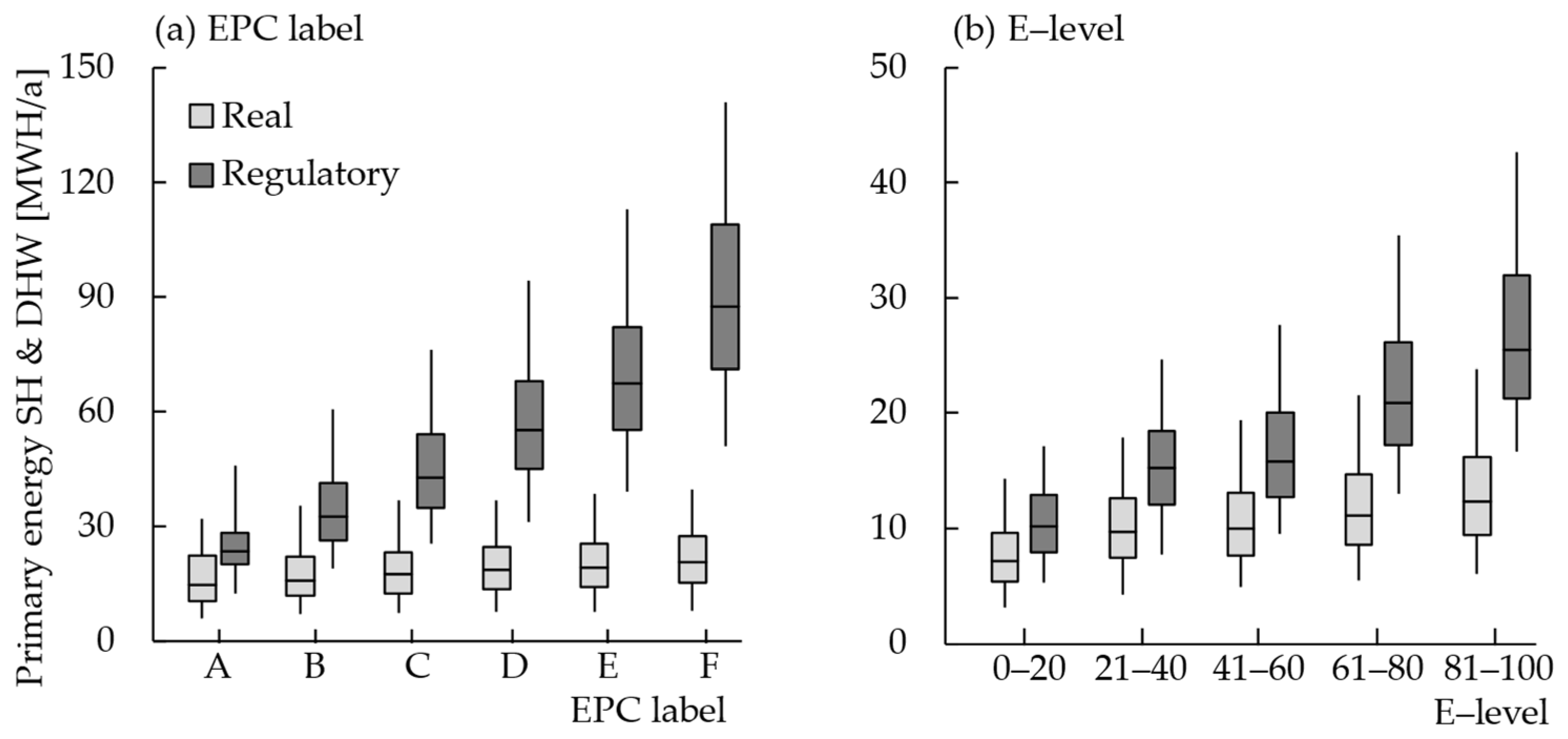
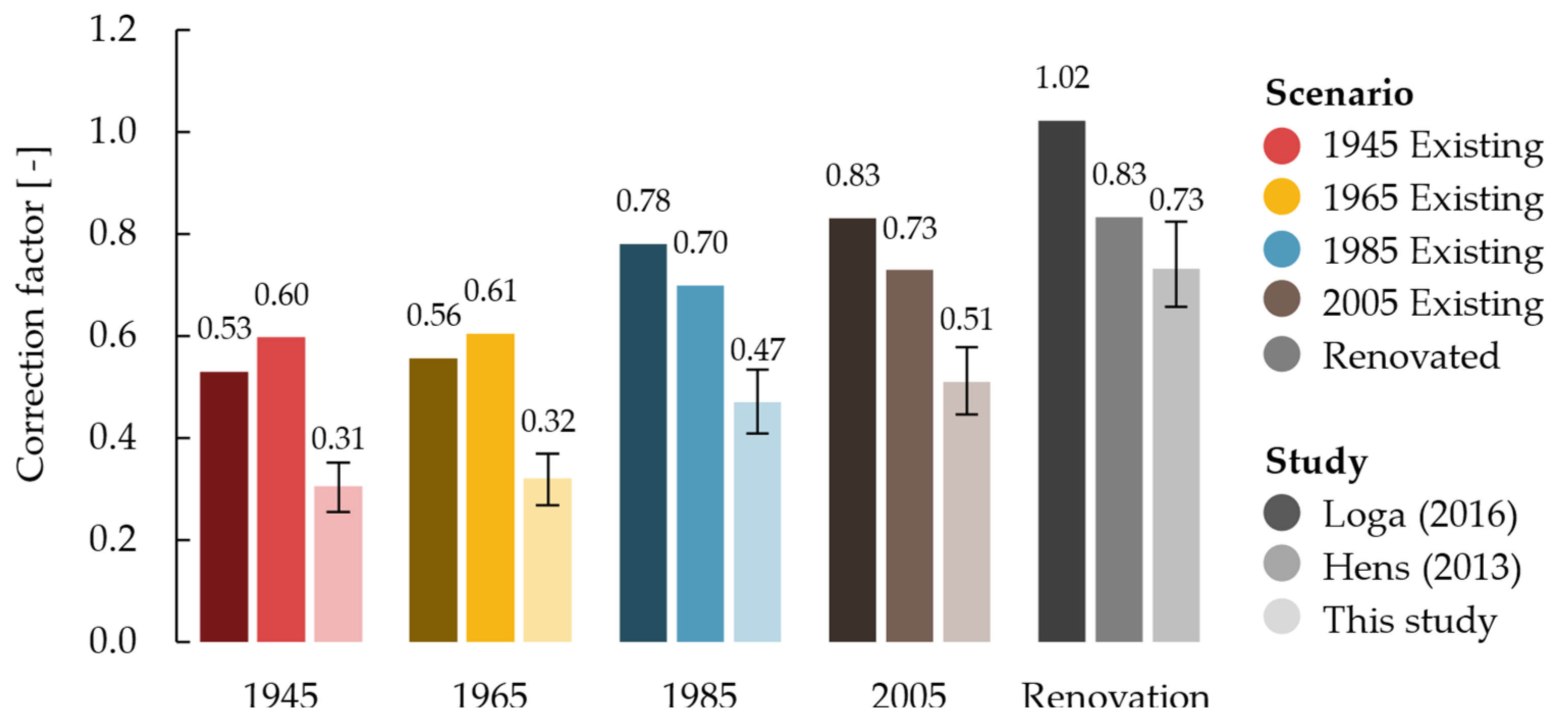
3.2. Correction Factors Per EPC Label and E-Level

The second step involves the definition of correction factors as a function of the EPC labels and E-levels, analogous to the approach applied by Tigchelaar et al. [61] and Laurent et al. [58]. First, the values for the 25th, 50th, and 75th percentiles of both actual and calculated energy use are derived from Figure 2 per EPC label and E-level. Subsequently, correction factors are determined by dividing the real energy use by the calculated energy use. The correction factors per EPC label and E-level are depicted in Figure 3.

A correction factor of one implies an equal actual and regulatory energy use, whereas a value below one indicates that actual energy use is lower than predicted. The correction factors based on median values (EPG50) range from 0.24 (EPC-label F) to 0.71 (E-level 0–20). The error bars represent results associated with the 25th and 75th percentiles, with a minimum of 0.21 for the 25th percentile and a maximum of 0.79 for the 75th percentile. These 25th and 75th percentile values are included in further steps to incorporate some spread on the EPG, representing high (EPG 25) and low correction (EPG75), respectively.

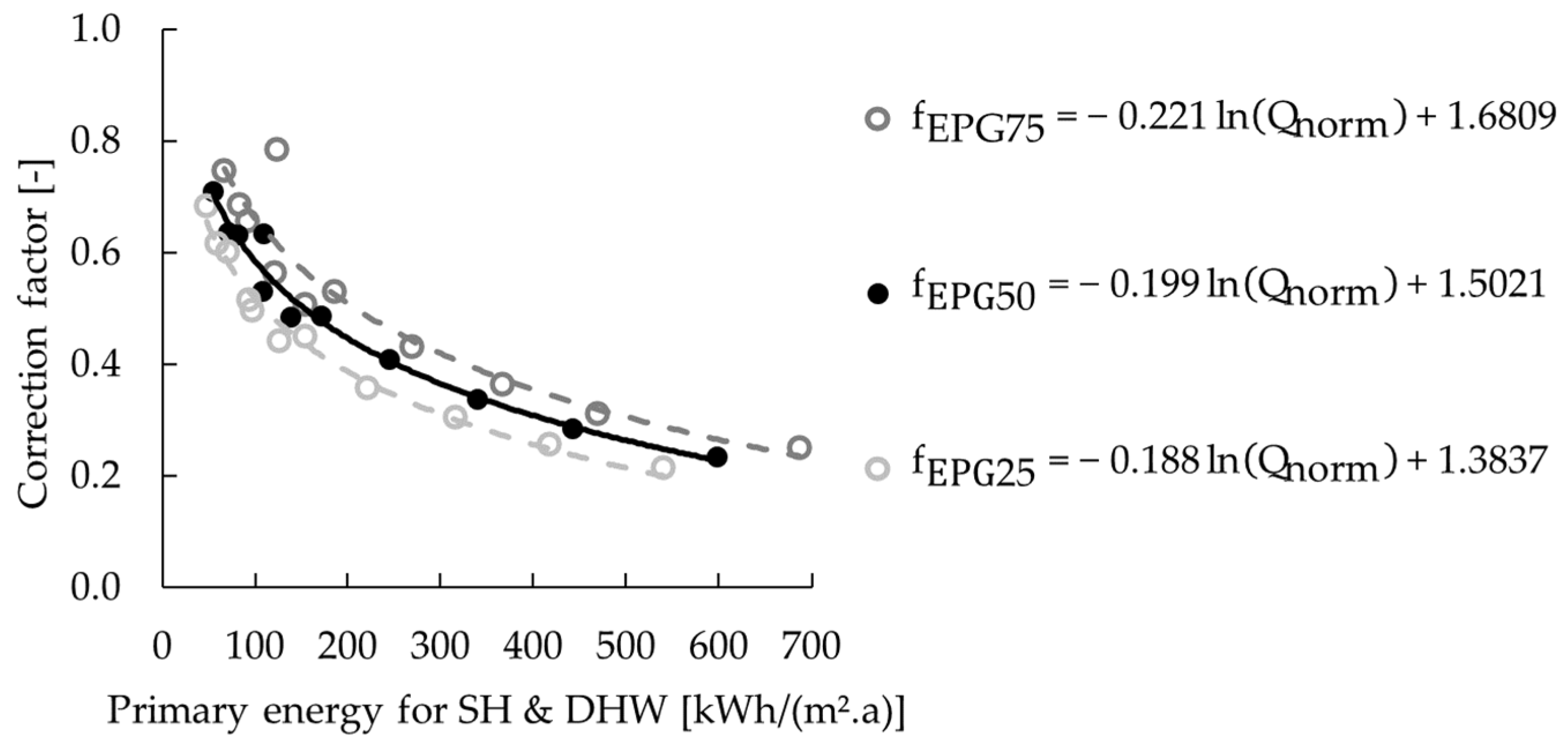
3.3. Correction Model as a Function of Normalized Primary Energy Use

In the third step, the findings obtained in the previous step are translated into a correction model that merges the factors from both datasets and deals with borderline cases. Specifically, cases that fall just within one category should not have a correction factor that significantly differs from cases falling just within another category. Therefore, each correction factor is linked to its corresponding normalized calculated energy use for space heating and DHW per gross floor area. These normalized values are documented in the research of Van Hove et al. [38,59]. For the high, median, and low correction factors, the values for the 25th, 50th, and 75th percentiles of normalized energy use, respectively, are gathered per EPC label and E-level, as listed in

Table 2. Normalized calculated energy use for the 25th, 50th, and 75th percentile correction factors per EPC label and E-level in kWh/(m².a) based on Van Hove et al. [38,59].

	EPC Labels						E-Levels
	A	B	C	D	E	F	0–20	21–40	41–60	61–80	81–100
25%	93	154	221	317	418	541	48	60	71	97	126
50%	109	172	245	340	442	598	55	72	81	108	139
75%	124	186	270	367	470	687	67	84	82	121	154

.

Subsequently, these normalized calculated energy uses are plotted against the correction factors established in the previous section, as illustrated in Figure 4.

A best-fit trend is sought among the data points, which is a logarithmic function. The obtained functions are also depicted in Figure 4, corresponding to the different percentile values. Moreover, it is assumed that real energy use never surpasses regulatory energy use due to the absence of data. For normalized calculated primary energy uses below 12.4 kWh/(m².a), it is suggested to apply a correction factor of one.

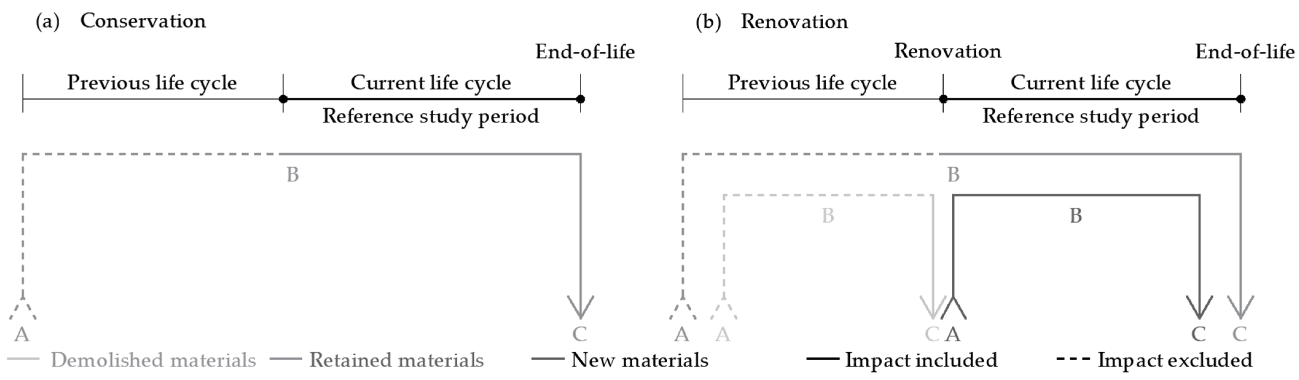
3.4. Integration into LCA Calculations

LCA considers both the embodied impact (i.e., raw material extraction, production, transport, construction, and end-of-life of materials) and operational energy use. The developed correction model only affects the latter, specifically, the regulatory calculated energy use for space heating and DHW. Using the normalized calculated primary energy use for space heating and DHW, low, median, and high correction factors are derived from the functions in Figure 4. These correction factors are applied to the regulatory calculated final energy use for space heating and DHW. The corrected final energy uses, along with other final energy uses (e.g., auxiliary energy), are then multiplied by the reference study period and the environmental impact of the respective energy source. This process results in the corrected environmental impact of operational energy use, which is added to the calculated embodied impact to obtain the total environmental impact.

$${EI}_{tot}={EI}_{emb}+\left[Q_{f, SH}·f_{EPG} · {EI}_{es}+Q_{f, DHW}·f_{EPG} · {EI}_{es}+\sum \left(Q_{f, other}· {EI}_{es}\right)\right]·RSP$$

(3)

with total environmental impact ${EI}_{tot}$ [Pt], embodied impact ${EI}_{emb}$ [Pt], final energy use for space heating $Q_{f, SH}$ [MJ/a], final energy use for DHW $Q_{f, DHW}$ [MJ/a], correction factor for EPG $f_{EPG}$ [-], other final energy uses $Q_{f, other}$ [MJ/a], environmental impact of energy source ${EI}_{es}$ [Pt/MJ], and reference study period $RSP$ [a].

4. Application of the Correction Model

The developed model is applied to four single-family dwellings characterized by an identical geometry but distinct construction years, with each initially exhibiting distinct energy characteristics. A description of the existing cases is provided in Section 4.1. Subsequently, these dwellings are energetically renovated to an identical energy performance in accordance with the current Flemish EPBD regulations, with the renovation scenarios elaborated in Section 4.2. Finally, the environmental impact of both the unrenovated and renovated buildings is quantified through LCA, as discussed in Section 4.3.

4.1. Description of Existing Dwellings

Four representative terraced single-family dwellings are considered, located in Flanders, Belgium. The dwellings share an identical geometry and floor plan (see Appendix A): a two-level main building of 6 by 9 m and a single-level horizontal extension of 3 by 3 m. The total gross floor area is 154 m², the volume is 490 m³, and the compactness is 2.1 m (i.e., ratio of volume to heat loss area based on external dimensions). However, the dwellings have different construction years of 1945, 1965, 1985, and 2005, with variations in construction method and insulation level. Representative building envelope elements for these construction years, together with their thermal characteristics, are derived from the Belgian residential building typologies from the TABULA/episcope project [67]. The composition and U-value for each envelope element are listed in Appendix A. None of the envelope elements of the two earlier construction years have any insulation, whereas varying degrees of insulation are present for the two later construction years. The average U-values are 3.0, 2.8, 1.1, and 0.9 W/(m².K) for the respective construction years. As TABULA provides little to no information regarding the materiality of the elements, assumptions are made about existing materials based on the research by Devos et al. [68].

Although the TABULA Webtool offers information on typical technical installations per construction period, this study assumes uniform installations across the four construction years. A condensing gas boiler with a 109.6% efficiency relative to the higher heating value is deployed for both space heating and DHW, with radiators at a temperature regime of 75/65 °C. Only natural ventilation is present, and poor airtightness is assumed for all existing states, considering a default v₅₀-value of 12 m³/(h.m²). No thermal bridge surcharge is considered due to the inadequate insulation level of the existing dwellings. The normalized primary energy uses are 410, 380, 182, and 150 kWh/(m².a). The first two dwellings have EPC-labels E and D, and the latter two both have EPC-label B.

4.2. Renovation Scenarios

These existing dwellings are renovated in an analogous way. All building envelope elements are insulated to such a degree that they meet the current maximum U-values imposed by the EPBD regulations for energy renovations in Flanders (i.e., 0.24 W/(m².K) for opaque elements, 1.50 W/(m².K) for windows, and 2.00 W/(m².K) for external doors). The average U-value of the building envelope after renovation is 0.38 W/(m².K).

One renovation strategy per envelope element is proposed, employing identical materials for the four dwellings. The external wall is insulated by gluing EPS to the outer surface of the existing structure, finished with an exterior plaster (ETICS). In dwellings with a cavity wall, the outer brick (and any existing insulation) is first removed. For the 1945 dwelling, the pitched roof is completely reconstructed (i.e., ceramic roof tiles, roof foil, glass wool between trusses, PE-foil, and gypsum board), whereas for the other dwellings, glass wool insulation is added between the existing structure, with PE-foil and gypsum board at the interior side. The existing interior finishing and insulation are again first removed. For the flat roofs, bitumen roofing and any existing insulation are removed, followed by the application of PUR insulation and EPDM on top of the existing concrete structure. Furthermore, the existing floor tiles and cement screed of the slab on grades are removed, after which PUR is sprayed onto the existing structure. Subsequently, PE-foil, new cement screed, and ceramic tiles are provided. Note that the 1945 dwelling has no concrete slab yet; therefore, a new reinforced concrete slab is additionally considered. Finally, the windows are replaced with high-efficiency double glazing in new PVC frames, and the external doors are upgraded to doors with a better thermal property.

Regarding technical installations, a new condensing gas boiler is implemented in all dwellings, with an efficiency identical to the existing one (i.e., 109.6% relative to the higher heating value). The radiators are replaced by low-temperature radiators operating at 50/40 °C. Furthermore, a balanced ventilation system with heat recovery (84% effectiveness) is installed. Moreover, an improvement in airtightness is assumed, characterized by a v₅₀-value of 6 m³/(h.m²). In addition, thermal bridges are addressed through a 0.04 W/(m².K) surplus on the average U-value of the envelope. The renovation results in a normalized primary energy use of 61 kWh/(m².a) for each dwelling.

4.3. LCA Method

To evaluate the environmental savings potential of renovating the four existing dwellings, an LCA is performed with the software SimaPro (v9.5). The study period is 60 years, which commences from the moment of renovation (here, 2025). This study period is in line with the Belgian LCA tool, TOTEM [69], and is commonly applied in the literature [70]. The functional unit is the conservation or renovation of an existing dwelling with a gross floor area of 154 m², encompassing both envelope materials and technical installations. Internal elements such as internal walls, floors, doors, and stairs are excluded from the analysis. The life cycle inventory utilizes generic data applicable to the European context, sourced from the Ecoinvent 3.9 ‘cut-off’ database. Furthermore, the EN 15978+A2 method is used with PEF (Product Environmental Footprint) normalization and weighting factors [71,72]. The results are aggregated into a single score, expressed in points (Pt).

The research includes the product (A1–3), construction (A4–5), replacement (B4), operational energy use (B6), and end-of-life (C1–4) stages. The embodied impact comprises all mentioned stages, excluding operational energy use. To assess the embodied impact of the building envelope, the impact of the 1 m² element is extrapolated to the building level. Regarding technical installations, the embodied impact includes the condensing gas boiler, radiators, air handling unit, air valves, and air ducting, of which the data inventory relies on prior research conducted by the authors [73]. Other components are excluded, as their embodied impact is assumed to remain constant across all scenarios. Assumptions to quantify the embodied impact (e.g., transport distances and end-of-life scenarios) are derived from the Belgian LCA tool, TOTEM [74], along with the approach to define the system boundaries for demolished, retained, and new materials, as shown in Figure 5. The replacement and end-of-life stages of existing materials are included, whereas only the end-of-life stage is considered for demolished materials.

Finally, the operational energy use (B6) is computed according to the national single-zone monthly quasi-steady-state method with a uniform interior temperature of 18 °C [66]. This includes space heating, DHW, and auxiliary energy; electricity use for lighting and appliances is excluded. Note that the correction model from Section 3 is exclusively applied to final energy use for space heating and DHW. The final energy use is multiplied with the 60-year study period and the environmental impact of gas (for space heating and DHW) and electricity (for auxiliary energy).

5. Results

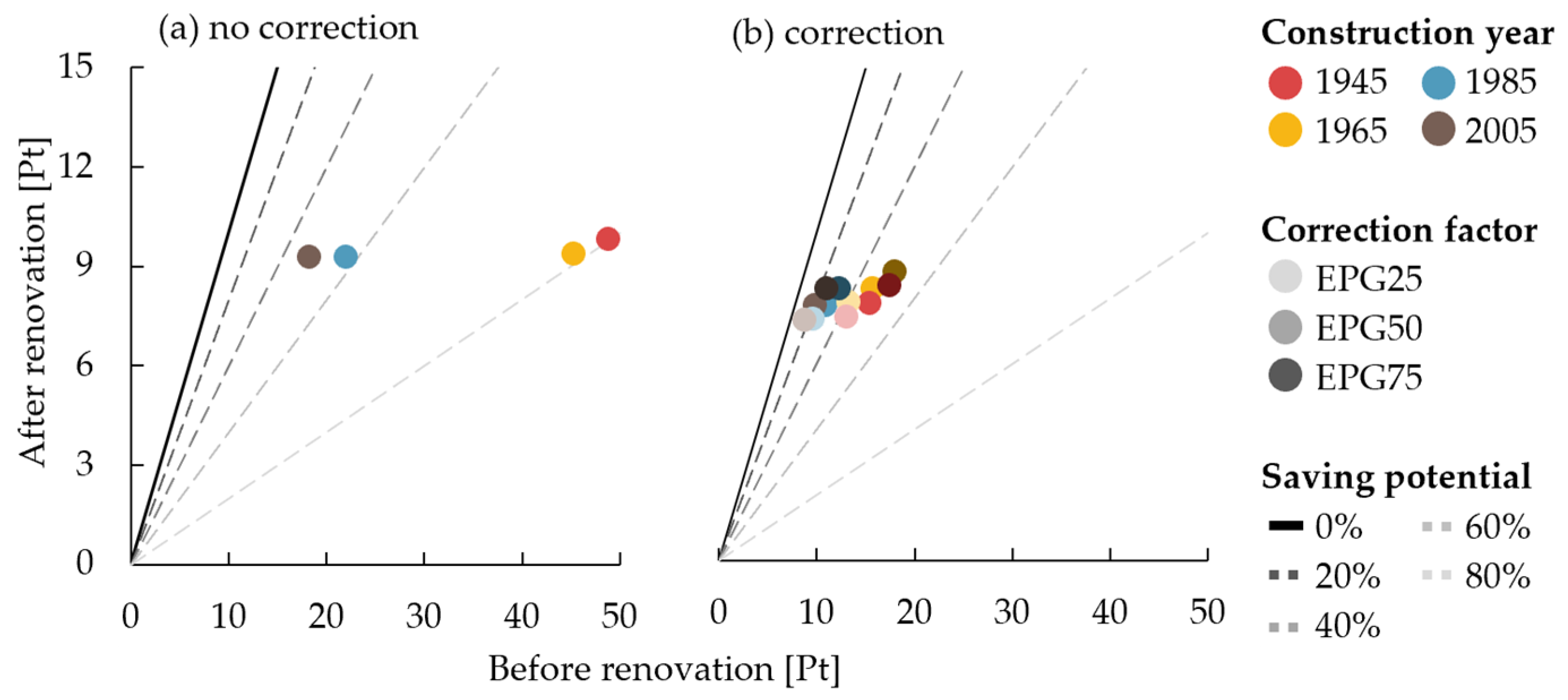
5.1. Environmental Savings Potential

This first section investigated the environmental savings potential of renovating the four existing dwellings. First, the effect of implementing the developed correction model on the environmental impact of operational energy use is assessed, neglecting the embodied impact. The operational environmental savings potential is calculated, defined as the disparity between the operational impact post-renovation and pre-renovation, expressed as a percentage relative to the operational impact pre-renovation.

Subsequently, these results are extended by including the embodied impact, thereby investigating the influence of the EPG on the overall life cycle environmental impact. Analogously, the life cycle environmental savings potential is determined. Similar to the definition of the operational environmental savings potential, the life cycle environmental savings potential is the percentage difference between the life cycle environmental impact after and before renovation, relative to the latter.

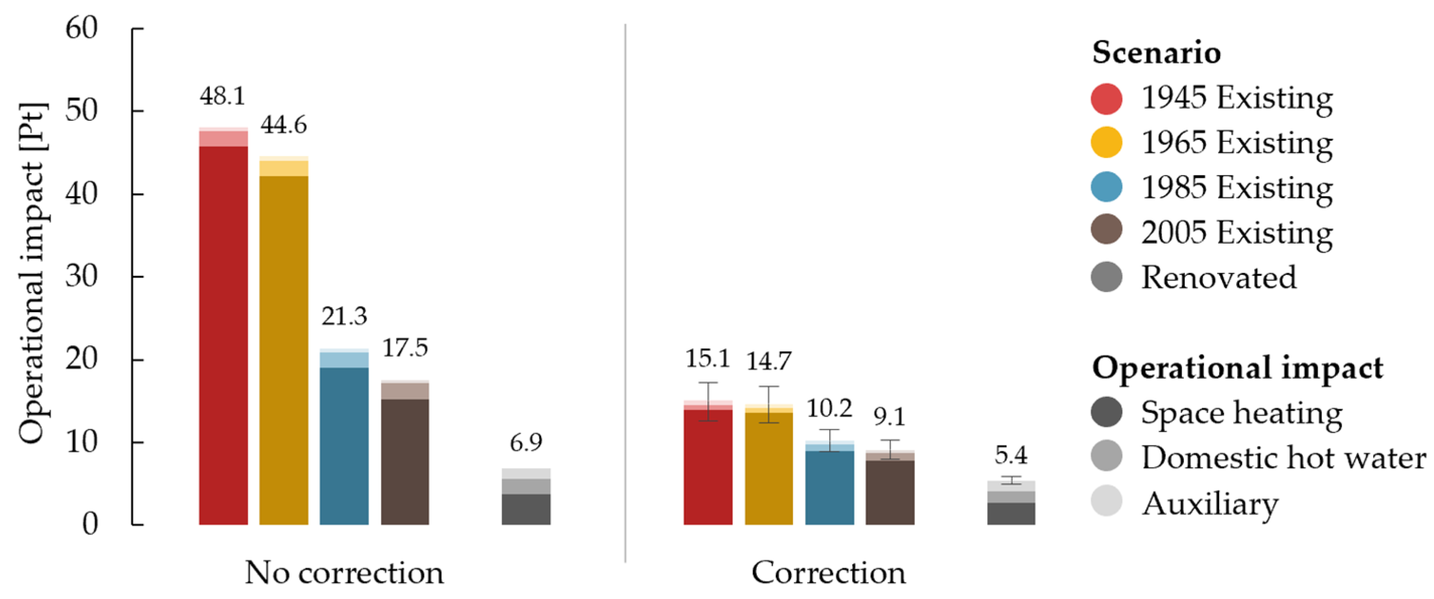
5.1.1. Operational Impact

The annual final energy uses for space heating, DHW, and auxiliary energy for the four existing cases and their renovated state are shown in

Table 3. Annual final energy use for space heating, domestic hot water, and auxiliary, in MJ.

	1945	1965	1985	2005	Renovation
Space heating	216,471	199,754	90,075	72,304	17,660
Domestic hot water	8830	8830	8830	8830	8830
Auxiliary energy	1022	996	774	721	2398

.

The final energy use for space heating and auxiliary energy of the unrenovated dwellings varies. The older the dwelling, the higher the final energy use before renovation. The final energy use for DHW is identical for all cases. Furthermore, renovating the four dwellings results in an equal final energy use, as all boundary conditions affecting energy use are identical.

Subsequently, correction factors for space heating and DHW are determined through the application of the established model. The values for space heating and DHW from Table 3 are enumerated and normalized by the gross floor area of 154.2 m² to obtain normalized final energy use per unit floor area. These values are converted into kWh by dividing them by 3.6 and multiplied with the primary conversion factor for gas, which equals 1. Based on the defined functions discussed in Section 3, the correction factors for the respective normalized primary energy uses are computed. The obtained correction factors, corresponding to the 25th, 50th, and 75th percentiles, are listed in

Table 4. High (EPG25), median (EPG50), and low (EPG75) correction factors to correct final energy use for space heating and domestic hot water in the existing and renovated dwellings.

	1945	1965	1985	2005	Renovation
EPG25	0.25	0.27	0.41	0.45	0.66
EPG50	0.31	0.32	0.47	0.51	0.73
EPG75	0.35	0.37	0.53	0.58	0.83

for the unrenovated and renovated dwellings. The median correction factors range from 0.31 (oldest, least energy efficient dwelling) to 0.73 (all renovated dwellings). As previously noted, the smaller the factor, the more pronounced the overestimation of the energy use.

Finally, these factors are applied to the final energy use for space heating and DHW, after which the results are translated into an environmental impact, together with the uncorrected auxiliary energy use, over a 60-year study period. The operational impact for the four unrenovated dwellings is depicted in Figure 6, juxtaposed with the operational impact after renovation, which is identical for all cases. The figure shows the outcomes for both the uncorrected and corrected operational impact. Moreover, the error bars reflect the application of the correction factors for the 25th and 75th percentiles.

In all scenarios, space heating dominates the operational impact. In the unrenovated dwellings, space heating constitutes 87–95% of the operational impact without correction, whereas DHW accounts for 4–11%. After renovation, the contribution of space heating notably decreases to 54%. Conversely, the share of DHW and auxiliary energy increases to 27% and 18%, respectively. In addition, the operational savings vary between 61% and 86% when no correction factors are applied. However, the application of the respective correction factors from Table 4 substantially reduces the savings potential to only 41–64%, with a margin of 1–4%.

5.1.2. Life Cycle Environmental Impact

Subsequently, Formula (3) is used to determine the corrected life cycle environmental impact before and after renovation per dwelling. Additionally, the uncorrected life cycle environmental impact is calculated by using a correction factor of one to exclude the EPG. This allows for the examination of the effect of the EPG on the life cycle environmental impact and environmental savings potential. The corrected and uncorrected operational impacts from the previous section are thus supplemented with the embodied impact of the building envelope and technical installations. The embodied impact encompasses necessary material replacements in the existing dwellings, along with the additional materials required for their renovation. The balance between the embodied and operational impact is shown in Figure 7.

Operational energy use comprises 70–99% of the life cycle environmental impact when no correction is considered (Figure 7a,c). Specifically, the operational energy contribution of the unrenovated existing dwellings spans from 96% to 99%, whereas for the renovated dwellings, the contribution is 70% to 74%. Implementing the median correction factors (EPG50) results in a reduction of these figures to 64–96% (Figure 7b,d). Due to the lower operational impact after correction, the embodied share proportionally increases, leading to a systematic underestimation of its significance. Specifically, the embodied impact is 1.2 to 3.1 times more significant than initially expected.

Subsequently, the environmental savings potential is discussed, which represents the relative difference between the life cycle environmental impact before and after renovation, relative to the former. Figure 8 shows the life cycle environmental impact before and after renovation for the different dwellings, without and with correction for the EPG. The diagonal lines indicate the environmental savings due to renovation.

Figure 8a shows the results without correction for the EPG, demonstrating environmental savings of 49–80%. The highest savings are realized through the renovation of the 1945 dwelling (80%), closely followed by the renovation of the 1965 dwelling (79%). Renovating the 1985 dwelling yields savings of 58%, whereas the savings potential for the 2005 dwelling is 49%. These savings are thus comparatively smaller than the operational savings (which were 61–86%), attributable to the inclusion of the embodied impact.

Similarly, Figure 8b shows the life cycle environmental impacts after the application of the high, median, and low correction factors in Formula (3). Evidently, correcting for the EPG significantly reduces the environmental savings, as the life cycle environmental impact is reduced more before renovation than after renovation. When considering median correction factors (EPG50), the savings are only 21–49% compared to the initial 49–80%. Moreover, the savings potential is 5–7% lower when incorporating high correction factors (EPG25) and 3–4% higher when considering low correction factors (EPG75). In conclusion, the discernible difference in savings potential underscores the importance of taking into account the EPG when assessing the environmental benefits of renovation.

In addition, these findings can be translated into an ‘environmental performance gap’, which can be defined analogously to the EPG as the difference between the uncorrected and corrected life cycle environmental impact, relative to the former. The outcomes indicate an environmental performance gap varying between 15% and 68%. The highest gap corresponds to the unrenovated 1945 dwelling, whereas the lowest gap is associated with the renovated 1945 dwelling. These figures are lower than the EPG (1—correction factor), ranging from 27% to 69%, due to the inclusion of the embodied impact.

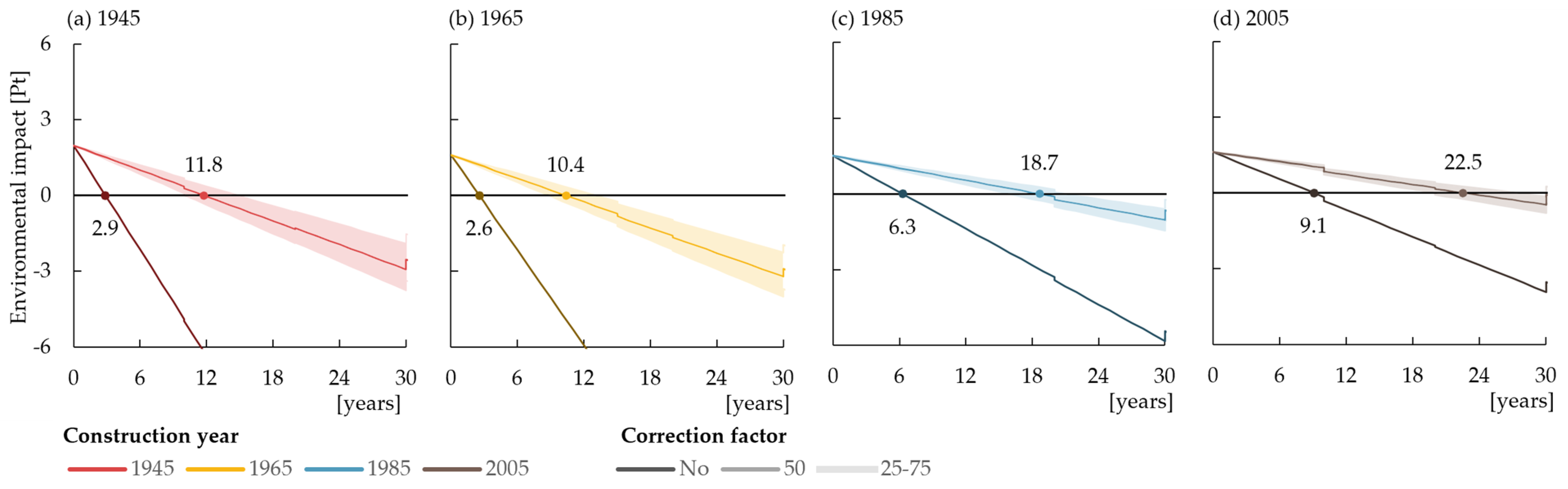
5.2. Environmental Payback Time

Finally, the effect of integrating the EPG through the proposed correction model on the environmental payback time (EPBT) is assessed. The EPBT is defined as the time required for the embodied impact to be offset by the annual operational energy savings. In other words, the EPBT represents the ratio of the embodied impact difference between the unrenovated and renovated building to the annual operational impact savings. Figure 9 illustrates the environmental impact calculated over time, with and without consideration of the EPG, for the four dwellings.

In year zero, the difference in embodied impact for production, transport, and construction between the unrenovated and renovated dwellings is depicted. Subsequent years show the gradual compensation of the initial embodied impact by annual operational energy savings, accounting for any material replacements required during renovation. The EPBT marks the point when the cumulative environmental impact equals zero.

The EPBT, without correction for the EPG, ranges from 2.9 to 9.1 years. The lowest EPBT corresponds to the renovated 1965 dwelling, closely followed by the renovated 1945 dwelling. Despite the higher annual operational energy savings for the 1945 dwelling, its renovation demands a greater amount of materials due to the complete reconstruction of the pitched roof and the casting of a new reinforced concrete slab, which is not required in the 1965 dwelling. The slightly higher EPBT for the 1945 dwelling is therefore attributed to the higher initial embodied impact, necessitating more time to be compensated for by the energy savings. Conversely, the highest EPBT corresponds to the renovation of the 2005 dwelling because of the smaller energy savings, which is associated with the better initial energy performance of the unrenovated dwelling.

When the median correction factors (EPG50) are considered, the EPBT considerably increases, ranging from 10.4 to 22.5 years. Moreover, Figure 9 additionally depicts the spread of these values by applying the high and low correction factors. The EPBT spans from 13.0 to 27.3 years for the high factors (EPG25) and from 8.8 to 19.9 years for the low factors (EPG75). Although these EPBTs are significantly higher than those observed without correction, they still fall within the considered 60-year study period.

6. Discussion

The objective of this paper was to address the EPG in LCA calculations and its implications for assessing the environmental savings and payback time of renovating single-family dwellings. To achieve this, a pragmatic, statistical correction model was developed to arrive at representative, average correction factors. The model was applied to four single-family dwellings with distinct energy characteristics, representative of the Flemish context. Their renovation involved quasi-identical strategies, resulting in an equal energy use after renovation. The environmental impact of both unrenovated and renovated dwellings was compared with and without the application of low, median, and high correction factors. This discussion section is first directed towards the developed correction model, after which the environmental savings and payback times are discussed.

6.1. Correction Model

First, the developed correction model is compared to existing models cited in Section 2. Tigchelaar et al. [61] and Laurent et al. [58] proposed correction factors based on EPC labels for Dutch, French, and English datasets. Tigchelaar et al. [61] reported factors between 0.53 and 0.88, whereas Laurent et al. [58] documented factors between 0.4 and 1.7. In this study, the median correction factors ranged from 0.24 to 0.63. A consistent trend across the correction factors is that real energy use in dwellings with worse EPC labels is substantially overestimated. This overestimation decreases as dwellings with better EPC labels are studied. Due to differences in national classification systems, comparing the factors per EPC label with the study’s results is not possible. However, the overall magnitude of the EPG in this study is significantly larger than in the other countries.

Loga et al. [39] and Hens [64] defined functions to correct calculated energy use. Applying these models to the present study’s dwellings shows that our correction factors are notably lower, particularly for the older, unrenovated dwellings (Figure 10). This disparity may stem from national variations, as Loga et al. [39] considered a German dataset; however, Hens [64] did focus on the Belgian context. Both prior studies exclusively considered space heating, whereas our study additionally accounted for DHW. The Flemish EPB method estimates the net energy use for DHW based on the building’s volume [66]. However, this approach might underestimate real energy use for DHW in small dwellings or overestimate it in large dwellings, as the size of the dwelling may not accurately reflect the number of occupants [75].

As demonstrated by Van de Putte et al. [76], who focused on two multi-family buildings, the Flemish EPB method can lead to a significant overestimation of energy use for DHW. The analysis showed that 97% and 98% of the apartment units exhibited actual energy use for DHW that was smaller than the calculated values. Notably, in a substantial portion of these units (81% and 85%), actual energy use was even less than half of the calculated values. In our study, DHW accounted for only 4–11% of the operational impact in the unrenovated dwellings but rose to 27% for the renovated dwellings. For unrenovated dwellings, the correction will thus be predominantly influenced by space heating, whereas for renovated dwellings, it remains uncertain whether space heating or DHW dominates the correction. Given the absence of separate data, considering the combined effect of both space heating and DHW is considered the most suitable for this study.

Furthermore, the developed correction model exhibits several limitations. The model relies on a recent, extensive Belgian study conducted by Van Hove et al. [38,59]. Consequently, the inherent limitations of their research apply to this study. For instance, data quality is a concern, particularly the accuracy of input data in energy performance certificates. The precision of these reported data was uncertain, as assessors’ choices might influence the resulting energy ratings. In addition, the actual figures for natural gas consumption might include domestic cooking, as dwellings with gas-based cooking could not be identified. Thus, the obtained correction factors might have exerted a slightly higher impact if these specific cases could have been excluded.

The proposed statistical model, which corrects energy use as a function of calculated normalized primary energy use, only limitedly captures the large variability in actual energy use for a given calculated energy use, as documented in the literature. This variability stems from diverse origins, including user behavior, climate conditions, building characteristics, and construction quality. To mitigate this limitation, low and high correction factors were included in addition to median correction factors. Moreover, the primary objective of this research was not to identify explanatory parameters but rather to integrate the EPG in a simplified manner into LCA calculations. Therefore, the focus was on providing a pragmatic correction model in which simplicity and flexibility were prioritized over the complexities of correcting physical modeling of buildings.

Lastly, the research aimed to address the importance of the EPG on the environmental savings potential and payback times of energy renovations, given the lack of studies integrating the EPG into LCA calculations. The present study does not focus on a specific real-world renovation project but instead considers a synthetic sample of representative cases. Therefore, an average correction based on large-scale statistical data was found most appropriate. Additionally, the model applicability is confined to the Belgian context, as the EPG varies across countries. However, the described methodology in Section 3 remains transferable, as similar datasets to those provided by Van Hove et al. [38,59] are available in other countries like Switzerland [35] and the Netherlands [36].

6.2. Environmental Savings Potential and Payback Times

The literature reports a broad range of environmental savings potential and payback times, though comparability is challenging due to differences in energy characteristics and renovation measures. Based on the results of our research, integrating the EPG in existing LCA studies is expected to significantly reduce reported environmental savings and considerably increase payback times. The latter was also concluded by Jerome et al. [77] when assessing the life cycle GWP of renovated and unrenovated buildings by means of calculated and measured energy savings. Whereas the payback time was 7.5 years based on calculated energy use, this value rose to 25 years when actual measured data were used.

Integrating the EPG did not nullify the environmental savings potential in our research; instead, corrected savings of 16–51% were observed compared to 49–80% without correction. Additionally, the corrected payback times of 8.9–27.4 years contrast with the uncorrected 2.9–9.1 years, yet still remain well within the expected service life of buildings. There is thus a potential environmental benefit of renovating dwellings; nevertheless, this benefit is highly contingent upon the actual energy use pre-renovation. Moreover, renovation should not be solely perceived as a means to achieve energy savings. It holds broader benefits, including enhancements in comfort, indoor air quality, health, social well-being, and market value [78,79,80].

Lastly, it must be noted that the results from this research regarding environmental savings and payback times are case-specific. Specifically, this research considered the renovation of four single-family dwellings with an identical geometry but varying construction years. Only one renovation strategy for the building envelope and technical installations was considered. However, as the research considered representative dwellings in Flanders, the results can be generalized and extrapolated to similar cases.

7. Conclusions

This study examined the effect of integrating the energy performance gap into the framework of the environmental impact assessments for building renovation. First, a statistical correction model was developed, which built on a large-scale study on the energy performance gap between real and regulatory calculated energy use of Flemish single-family dwellings. This model provides a logarithmic function contingent upon normalized primary energy use for space heating and domestic hot water. It offers a pragmatic approach to address the energy performance gap in LCA calculations for renovation projects, acknowledging its limitations and contextual constraints.

Upon applying the correction model to four representative Flemish single-family dwellings, the environmental savings decreased by 28–31%, and the environmental payback times increased by 7.5 to 13.4 years. Due to correction, the share of operational energy use in the life cycle environmental impact significantly decreased, thereby amplifying the relative contribution of materials. This trend leads to a systematic underestimation of the significance of material choices in renovation projects. These findings underscore the importance of integrating the energy performance gap into LCA calculations to more accurately assess the potential environmental benefits of building renovations. The developed model enhances the reliability of LCA outcomes, supports informed decision making for sustainable building practices, and aids in providing a more realistic estimation of the environmental savings associated with renovating the existing building stock.

In conclusion, it is strongly recommended to rectify energy use calculations derived from regulatory methods in comparative LCAs between unrenovated and renovated dwellings. The actual energy use, especially in the case of existing inadequately or non-insulated dwellings, proves to be significantly lower than the calculated energy use, thereby resulting in a non-negligible overestimation of predicted savings potential. This overestimation, coupled with the inclusion of the embodied impact in a life cycle approach in addition to operational energy use, reduces the ecological benefit of renovation. Therefore, it is recommended to rely on measured data whenever possible to evaluate the environmental advantages of renovation more realistically. However, when measured data are not available, it is advisable to correct regulatory calculated energy uses by means of correction factors, as explored in this study. Future research can build on the proposed model to explore region-specific adjustments and further refine it to include other building types.

References

1. European Commission. Going Climate-Neutral by 2050—A Strategic Long-Term Vision for a Prosperous, Modern, Competitive and Climate-Neutral EU Economy; European Commission: Brussels, Belgium, 2019.
2. European Commission. Stepping up Europe’s 2030 Climate Ambition: Investing in a Climate-Neutral Future for the Benefit of Our People; European Commission: Brussels, Belgium, 2020.
3. European Commission. A Renovation Wave for Europe—Greening Our Buildings, Creating Jobs, Improving Lives; European Commission: Brussels, Belgium, 2020.
4. BPIE. Deep Renovation: Shifting from Exception to Standard Practice in EU Policy; Buildings Performance Institute Europe (BPIE): Brussels, Belgium, 2021. [Google Scholar]
5. BPIE. How to Stay Warm and Save Energy: Insulation Opportunities in European Homes; Buildings Performance Institute Europe (BPIE): Brussels, Belgium, 2023. [Google Scholar]
6. Dominguez, C.; Kakkos, E.; Gross, D.; Hischier, R.; Orehounig, K. Renovated or Replaced? Finding the Optimal Solution for an Existing Building Considering Cumulative CO2 Emissions, Energy Consumption and Costs—A Case Study. Energy Build. 2024, 303, 113767. [Google Scholar] [CrossRef]
7. Passer, A.; Ouellet-Plamondon, C.; Kenneally, P.; John, V.; Habert, G. The Impact of Future Scenarios on Building Refurbishment Strategies towards plus Energy Buildings. Energy Build. 2016, 124, 153–163. [Google Scholar] [CrossRef]
8. Conci, M.; Konstantinou, T.; van den Dobbelsteen, A.; Schneider, J. Trade-off between the Economic and Environmental Impact of Different Decarbonisation Strategies for Residential Buildings. Build. Environ. 2019, 155, 137–144. [Google Scholar] [CrossRef]
9. Chandrasekaran, V.; Dvarioniene, J.; Vitkute, A.; Gecevicius, G. Environmental Impact Assessment of Renovated Multi-Apartment Building Using LCA Approach: Case Study from Lithuania. Sustainability 2021, 13, 1542. [Google Scholar] [CrossRef]
10. de Oliveira Fernandes, M.A.; Keijzer, E.; van Leeuwen, S.; Kuindersma, P.; Melo, L.; Hinkema, M.; Gonçalves Gutierrez, K. Material-versus Energy-Related Impacts: Analysing Environmental Trade-Offs in Building Retrofit Scenarios in the Netherlands. Energy Build. 2021, 231, 110650. [Google Scholar] [CrossRef]
11. Vavanou, A.; Schwartz, Y.; Mumovic, D. The Life Cycle Impact of Refurbishment Packages on Residential Buildings with Different Initial Thermal Conditions. J. Hous. Built Environ. 2022, 37, 951–1000. [Google Scholar] [CrossRef]
12. González-Prieto, D.; Fernández-Nava, Y.; Marañón, E.; Prieto, M.M. Environmental Life Cycle Assessment Based on the Retrofitting of a Twentieth-Century Heritage Building in Spain, with Electricity Decarbonization Scenarios. Build. Res. Inf. 2021, 49, 859–877. [Google Scholar] [CrossRef]
13. Apostolopoulos, V.; Mamounakis, I.; Seitaridis, A.; Tagkoulis, N.; Kourkoumpas, D.S.; Iliadis, P.; Angelakoglou, K.; Nikolopoulos, N. An Integrated Life Cycle Assessment and Life Cycle Costing Approach towards Sustainable Building Renovation via a Dynamic Online Tool. Appl. Energy 2023, 334, 120710. [Google Scholar] [CrossRef]
14. Struhala, K.; Ostrý, M. Life-Cycle Assessment of a Rural Terraced House: A Struggle with Sustainability of Building Renovations. Energies 2021, 14, 2472. [Google Scholar] [CrossRef]
15. Rabani, M.; Madessa, H.B.; Ljungström, M.; Aamodt, L.; Løvvold, S.; Nord, N. Life Cycle Analysis of GHG Emissions from the Building Retrofitting: The Case of a Norwegian Office Building. Build. Environ. 2021, 204, 108159. [Google Scholar] [CrossRef]
16. Khadra, A.; Akander, J.; Myhren, J.A. Greenhouse Gas Payback Time of Different HVAC Systems in the Renovation of Nordic District-Heated Multifamily Buildings Considering Future Energy Production Scenarios. Buildings 2024, 14, 413. [Google Scholar] [CrossRef]
17. Arbulu, M.; Oregi, X.; Etxepare, L. Parametric Simulation Tool for the Enviro-Economic Evaluation of Energy Renovation Strategies in Residential Buildings with Life Cycle Thinking: PARARENOVATE-LCT. Energy Build. 2024, 312, 114182. [Google Scholar] [CrossRef]
18. Rasmussen, F.N.; Birgisdottir, H. Life Cycle Environmental Impacts from Refurbishment Projects—A Case Study. In Proceedings of the CESB2016: Innovations for Sustainable Future, Prague, Czech Republic, 22–24 June 2016; pp. 277–284. [Google Scholar]
19. Shirazi, A.; Ashuri, B. Embodied Life Cycle Assessment (LCA) Comparison of Residential Building Retrofit Measures in Atlanta. Build. Environ. 2020, 171, 106644. [Google Scholar] [CrossRef]
20. Dodoo, A.; Gustavsson, L.; Sathre, R. Life Cycle Primary Energy Implication of Retrofitting a Wood-Framed Apartment Building to Passive House Standard. Resour. Conserv. Recycl. 2010, 54, 1152–1160. [Google Scholar] [CrossRef]
21. Lasvaux, S.; Favre, D.; Périsset, B.; Bony, J.; Hildbrand, C.; Citherlet, S. Life Cycle Assessment of Energy Related Building Renovation: Methodology and Case Study. Energy Procedia 2015, 78, 3496–3501. [Google Scholar] [CrossRef]
22. Ramírez-Villegas, R.; Eriksson, O.; Olofsson, T. Life Cycle Assessment of Building Renovation Measures–Trade-off between Building Materials and Energy. Energies 2019, 12, 344. [Google Scholar] [CrossRef]
23. Asdrubali, F.; Ballarini, I.; Corrado, V.; Evangelisti, L.; Grazieschi, G.; Guattari, C. Energy and Environmental Payback Times for an NZEB Retrofit. Build. Environ. 2019, 147, 461–472. [Google Scholar] [CrossRef]
24. Zhang, C.; Hu, M.; Laclau, B.; Garnesson, T.; Yang, X.; Tukker, A. Energy-Carbon-Investment Payback Analysis of Prefabricated Envelope-Cladding System for Building Energy Renovation: Cases in Spain, the Netherlands, and Sweden. Renew. Sust. Energ. Rev. 2021, 145, 111077. [Google Scholar] [CrossRef]
25. Wrålsen, B.; O’Born, R.; Skaar, C. Life Cycle Assessment of an Ambitious Renovation of a Norwegian Apartment Building to NZEB Standard. Energy Build. 2018, 177, 197–206. [Google Scholar] [CrossRef]
26. Decorte, Y.; Steeman, M.; Van Den Bossche, N.; Calle, K. Environmental Evaluation of Pareto Optimal Renovation Strategies: A Multidimensional Life-Cycle Analysis. In Proceedings of the E3S Web of Conferences, Tallinn, Estonia, 7–9 September 2020; Volume 172, p. 18003. [Google Scholar]
27. Van de moortel, E.; Allacker, K.; De Troyer, F.; Schoofs, E.; Stijnen, L. Dynamic Versus Static Life Cycle Assessment of Energy Renovation for Residential Buildings. Sustainability 2022, 14, 6838. [Google Scholar] [CrossRef]
28. Galimshina, A.; Moustapha, M.; Hollberg, A.; Padey, P.; Lasvaux, S.; Sudret, B.; Habert, G. What Is the Optimal Robust Environmental and Cost-Effective Solution for Building Renovation? Not the Usual One. Energy Build. 2021, 251, 111329. [Google Scholar] [CrossRef]
29. Galimshina, A.; Moustapha, M.; Hollberg, A.; Padey, P.; Lasvaux, S.; Sudret, B.; Habert, G. Statistical Method to Identify Robust Building Renovation Choices for Environmental and Economic Performance. Build. Environ. 2020, 183, 107143. [Google Scholar] [CrossRef]
30. Deurinck, M. Energy Saving Predictions in the Residential Building Sector: An Assessment Based on Stochastic Modeling. Ph.D. Thesis, KU Leuven, Leuven, Belgium, 2015. [Google Scholar]
31. van den Brom, P.; Meijer, A.; Visscher, H. Actual Energy Saving Effects of Thermal Renovations in Dwellings—Longitudinal Data Analysis Including Building and Occupant Characteristics. Energy Build. 2019, 182, 251–263. [Google Scholar] [CrossRef]
32. Hens, H. Energy Efficient Retrofit of an End of the Row House: Confronting Predictions with Long-Term Measurements. Energy Build. 2010, 42, 1939–1947. [Google Scholar] [CrossRef]
33. Rogan, F.; Gallachóir, B. Ex-Post Evaluation of a Residential Energy Efficiency Policy. In Proceedings of the ECEEE 2011 Summer Study, Belambra Presqu’île de Giens, France,, 6–11 June 2011; pp. 769–1778. [Google Scholar]
34. Vivian, J.; Carnieletto, L.; Cover, M.; De Carli, M. At the Roots of the Energy Performance Gap: Analysis of Monitored Indoor Air before and after Building Retrofits. Build. Environ. 2023, 246, 110914. [Google Scholar] [CrossRef]
35. Cozza, S.; Chambers, J.; Deb, C.; Scartezzini, J.L.; Schlüter, A.; Patel, M.K. Do Energy Performance Certificates Allow Reliable Predictions of Actual Energy Consumption and Savings? Learning from the Swiss National Database. Energy Build. 2020, 224, 110235. [Google Scholar] [CrossRef]
36. Majcen, D.; Itard, L.C.M.; Visscher, H. Theoretical vs. Actual Energy Consumption of Labelled Dwellings in the Netherlands: Discrepancies and Policy Implications. Energy Policy 2013, 54, 125–136. [Google Scholar] [CrossRef]
37. van den Brom, P.; Meijer, A.; Visscher, H. Performance Gaps in Energy Consumption: Household Groups and Building Characteristics. Build. Res. Inf. 2018, 46, 54–70. [Google Scholar] [CrossRef]
38. Van Hove, M.Y.C.; Deurinck, M.; Lameire, W.; Laverge, J.; Janssens, A.; Delghust, M. Large-Scale Statistical Analysis and Modelling of Real and Regulatory Total Energy Use in Existing Single-Family Houses in Flanders. Build. Res. Inf. 2023, 51, 203–222. [Google Scholar] [CrossRef]
39. Loga, T.; Stain, B.; Diefenbach, N.; Born, R. Deutsche Wohngebäudetypologie: Beispielhafte Maßnahmen Zur Verbesserung Der Energieeffizienz von Typischen Wohngebäuden; Institut Wohnen und Umwelt (IWU): Darmstadt, Germany, 2015. [Google Scholar]
40. Sunikka-Blank, M.; Galvin, R. Introducing the Prebound Effect: The Gap between Performance and Actual Energy Consumption. Build. Res. Inf. 2012, 40, 260–273. [Google Scholar] [CrossRef]
41. Mahdavi, A.; Berger, C.; Amin, H.; Ampatzi, E.; Andersen, R.K.; Azar, E.; Barthelmes, V.M.; Favero, M.; Hahn, J.; Khovalyg, D.; et al. The Role of Occupants in Buildings’ Energy Performance Gap: Myth or Reality? Sustainability 2021, 13, 3146. [Google Scholar] [CrossRef]
42. Zheng, Z.; Zhou, J.; Zhu, J.; Yang, Y.; Xu, F.; Liu, H. Review of the Building Energy Performance Gap from Simulation and Building Lifecycle Perspectives: Magnitude, Causes and Solutions. Dev. Built Environ. 2024, 17, 100345. [Google Scholar] [CrossRef]
43. Bai, Y.; Yu, C.; Pan, W. Systematic Examination of Energy Performance Gap in Low-Energy Buildings. Renew. Sustain. Energy Rev. 2024, 202, 114701. [Google Scholar] [CrossRef]
44. Cozza, S.; Chambers, J.; Brambilla, A.; Patel, M.K. In Search of Optimal Consumption: A Review of Causes and Solutions to the Energy Performance Gap in Residential Buildings. Energy Build. 2021, 249, 111253. [Google Scholar] [CrossRef]
45. van Dronkelaar, C.; Dowson, M.; Spataru, C.; Mumovic, D. A Review of the Regulatory Energy Performance Gap and Its Underlying Causes in Non-Domestic Buildings. Front. Mech. Eng. 2016, 1, 177335. [Google Scholar] [CrossRef]
46. Bakaloglou, S.; Charlier, D. The Role of Individual Preferences in Explaining the Energy Performance Gap. Energy Econ. 2021, 104, 105611. [Google Scholar] [CrossRef]
47. Khoury, J.; Alameddine, Z.; Hollmuller, P. Understanding and Bridging the Energy Performance Gap in Building Retrofit. Energy Procedia 2017, 122, 217–222. [Google Scholar] [CrossRef]
48. Lambie, E.; Saelens, D. Identification of the Building Envelope Performance of a Residential Building: A Case Study. Energies 2020, 13, 2469. [Google Scholar] [CrossRef]
49. La Fleur, L.; Moshfegh, B.; Rohdin, P. Measured and Predicted Energy Use and Indoor Climate before and after a Major Renovation of an Apartment Building in Sweden. Energy Build. 2017, 146, 98–110. [Google Scholar] [CrossRef]
50. Gupta, R.; Kapsali, M. Evaluating the ‘as-Built’ Performance of an Eco-Housing Development in the UK. Build. Serv. Eng. Res. Technol. 2016, 37, 220–242. [Google Scholar] [CrossRef]
51. Calì, D.; Osterhage, T.; Streblow, R.; Müller, D. Energy Performance Gap in Refurbished German Dwellings: Lesson Learned from a Field Test. Energy Build. 2016, 127, 1146–1158. [Google Scholar] [CrossRef]
52. Eon, C.; Breadsell, J.K.; Byrne, J.; Morrison, G.M. The Discrepancy between As-Built and As-Designed in Energy Efficient Buildings: A Rapid Review. Sustainability 2020, 12, 6372. [Google Scholar] [CrossRef]
53. Kaminska, A. Impact of Heating Control Strategy and Occupant Behavior on the Energy Consumption in a Building with Natural Ventilation in Poland. Energies 2019, 12, 4304. [Google Scholar] [CrossRef]
54. Charlier, D. Explaining the Energy Performance Gap in Buildings with a Latent Profile Analysis. Energy Policy 2021, 156, 112480. [Google Scholar] [CrossRef]
55. Brøgger, M.; Bacher, P.; Madsen, H.; Wittchen, K.B. Estimating the Influence of Rebound Effects on the Energy-Saving Potential in Building Stocks. Energy Build. 2018, 181, 62–74. [Google Scholar] [CrossRef]
56. Massié, C.; Belaïd, F. Estimating the Direct Rebound Effect for Residential Electricity Use in Seventeen European Countries: Short and Long-Run Perspectives. Energy Econ. 2024, 134, 107571. [Google Scholar] [CrossRef]
57. Galvin, R. The Economic Losses of Energy-Efficiency Renovation of Germany’s Older Dwellings: The Size of the Problem and the Financial Challenge It Presents. Energy Policy 2024, 184, 113905. [Google Scholar] [CrossRef]
58. Laurent, M.-H.; Galvin, R.; Oreszczyn, T.; Tigchelaar, C.; Allibe, B.; Hamilton, I. Back to Reality: How Domestic Energy Efficiency Policies in Four European Countries Can Be Improved by Using Empirical Data Instead of Normative Calculation. In Proceedings of the ECEEE 2013 Summer Study, Belambra Les Criques, France, 3–8 June 2013; pp. 2057–2070. [Google Scholar]
59. Van Hove, M. Increasing Reliability of Bottom-up Building-Stock Energy Models Using Available Data-Driven Techniques. Ph.D. Thesis, Ghent University, Ghent, Belgium, 2023. [Google Scholar]
60. Statbel Kadastrale Statistiek van Het Gebouwenpark. Available online: https://bestat.statbel.fgov.be/ (accessed on 12 June 2024).
61. Tigchelaar, C.; Daniëls, B.; Menkveld, M. Obligations in the Existing Housing Stock: Who Pays the Bills? In Proceedings of the ECEEE 2011 Summer Study, Belambra Presqu’île de Giens, France, 6–11 June 2011; pp. 353–363. [Google Scholar]
62. Cayre, E.; Allibe, B.; Laurent, M.-H.; Osso, D. There Are People in the House! How the Results of Purely Technical Analysis of Residential Energy Consumption Are Misleading for Energy Policies. In Proceedings of the ECEEE 2021 Summer Study, Belambra Presqu’île de Giens, France, 6–11 June 2011; pp. 1675–1683. [Google Scholar]
63. Van Droogenbroeck, K. Is EPC-Score D Eigenlijk H? Vlaamse Waarden Zijn Opvallend Soepeler Dan in Buurlanden; DPG Media: Antwerp, Belgium, 2020. [Google Scholar]
64. Hens, H. Human Habits and Energy Consumption in Residential Buildings; Scribd: San Francisco, CA, USA, 2013. [Google Scholar]
65. Flemish Energy and Climate Agency. Formulestructuur: Energiepresetatiecertificaat Bestaande Gebouwen Met Residentiële En Kleine Niet-Residentiele Bestemming; Flemish Energy and Climate Agency: Brussels, Belgium, 2022.
66. Flemish Energy Agency. Bijlage V: Bepalingsmethode van Het Peil van Primair Energieverbruik van Residentiële Eenheden; Flemish Energy Agency: Brussels, Belgium, 2022.
67. TABULA WebTool. Available online: https://webtool.building-typology.eu/#bm (accessed on 28 May 2024).
68. Devos, K.; Devlieger, L.; Steeman, M. Urban Mining: Availability of Building Materials in Flemish Social Housing Dwellings. In Proceedings of the 2nd International Conference on Construction, Energy, Environment & Sustainability, Funchal, Portugal, 27–30 June 2023. [Google Scholar]
69. OVAM TOTEM: Tool to Optimise the Total Environmental Impact of Materials. Available online: https://www.totem-building.be/ (accessed on 10 May 2024).
70. Dahiya, D.; Laishram, B. Life Cycle Energy Analysis of Buildings: A Systematic Review. Build. Environ. 2024, 252, 111160. [Google Scholar] [CrossRef]
71. Sala, S.; Cerutti, A.; Pant, R. Development of a Weighting Approach for the Environmental Footprint; Publications Office of the European Union: Luxembourg, 2017. [Google Scholar]
72. Sala, S.; Crenna, E.; Secchi, M.; Pant, R. Global Normalisation Factors for the Environmental Footprint and Life Cycle Assessment; Publications Office of the European Union: Luxembourg, 2017. [Google Scholar]
73. Decorte, Y.; Van Den Bossche, N.; Steeman, M. Importance of Technical Installations in Whole-Building LCA: Single-Family Case Study in Flanders. Build. Environ. 2024, 250, 111209. [Google Scholar] [CrossRef]
74. Trigaux, D.; Lam, W.C. Environmental Profile of Buildings [Update 2023]; OVAM: Mechelen, Belgium, 2023. [Google Scholar]
75. Allacker, K. Sustainable Building: The Development of an Evaluation Method. Ph.D. Thesis, KU Leuven, Leuven, Belgium, 2010. [Google Scholar]
76. Van De Putte, S.; Bracke, W.; Delghust, M.; Steeman, M.; Janssens, A. Comparison of the Actual and Theoretical Energy Use in NZEB Renovations of Multi-Family Buildings Using in Situ Monitoring. In Proceedings of the E3S Web Conference, Tallinn, Estonia, 7–9 September 2020. [Google Scholar]
77. Jerome, A.; Femenías, P.; Thuvander, L.; Wahlgren, P.; Johansson, P. Exploring the Relationship between Environmental and Economic Payback Times, and Heritage Values in an Energy Renovation of a Multi-Residential Pre-War Building. Heritage 2021, 4, 3652–3675. [Google Scholar] [CrossRef]
78. Popescu, D.; Bienert, S.; Schützenhofer, C.; Boazu, R. Impact of Energy Efficiency Measures on the Economic Value of Buildings. Appl. Energy 2012, 89, 454–463. [Google Scholar] [CrossRef]
79. Damen, S. Het Effect van Het EPC En Energetische Kenmerken Op de Verkoopprijs van Woningen in Vlaanderen; KU Leuven: Leuven, Belgium, 2019. [Google Scholar]
80. Pedersen, E.; Gao, C.; Wierzbicka, A. Tenant Perceptions of Post-Renovation Indoor Environmental Quality in Rental Housing: Improved for Some, but Not for Those Reporting Health-Related Symptoms. Build. Environ. 2021, 189, 107520. [Google Scholar] [CrossRef]
Figure 1. Steps in the development of the correction model with selection of dataset from Van Hove et al. [38,59].
Sustainability 16 07792 g001
Figure 2. Real and regulatory primary energy use for space heating (SH) and domestic hot water (DHW) per (a) EPC label for existing dwellings (n = 37,412) and (b) E-level for new dwellings (n = 49,781), adopted from Van Hove et al. [38,59].
Sustainability 16 07792 g002
Figure 3. Correction factors for the 25, 50, and 75th percentiles per (a) EPC label and (b) E-level, calculated with data derived from Van Hove et al. [38,59].
Sustainability 16 07792 g003
Figure 4. Correction factors for the 25th, 50th, and 75th percentiles as a function of normalized primary energy use for space heating (SH) and domestic hot water (DHW).
Sustainability 16 07792 g004
Figure 5. System boundaries for demolished, retained, and new materials in line with TOTEM [73] for (a) conservation and (b) renovation of an existing building.
Sustainability 16 07792 g005
Figure 6. Operational impact of the four dwellings with distinct construction years before and after renovation and with or without correction for the energy performance gap. The error bars reflect the application of the correction factors for the 25th and 75th percentiles.
Sustainability 16 07792 g006
Figure 7. Ratio of embodied and operational impact for the four dwellings with distinct construction years (a) pre-renovation without correction, (b) pre-renovation without correction, (c) post-renovation with correction, and (d) post-renovation with correction.
Sustainability 16 07792 g007
Figure 8. Life cycle environmental impact before and after renovation (a) without and (b) with high (EPG25), median (EPG50), and low (EPG75) correction for the energy performance gap.
Sustainability 16 07792 g008
Figure 9. Effect of applying the correction factors (50th, 25th, and 75th percentile) for the energy performance gap on the environmental payback time for dwellings with construction years of (a) 1945, (b) 1965, (c) 1985, and (d) 2005.
Sustainability 16 07792 g009
Figure 10. Comparison of correction factors derived from the developed model in this research with those from the models proposed by Loga et al. [39] and Hens [64], applied to the different existing and renovated dwellings.
Sustainability 16 07792 g010