
Invasive-Weed-Optimization-Based Extreme Learning Machine for Prediction of Lake Water Level Using Major Atmospheric–Oceanic Climate Scenarios


Abstract
1. Introduction
2. Materials and Methods
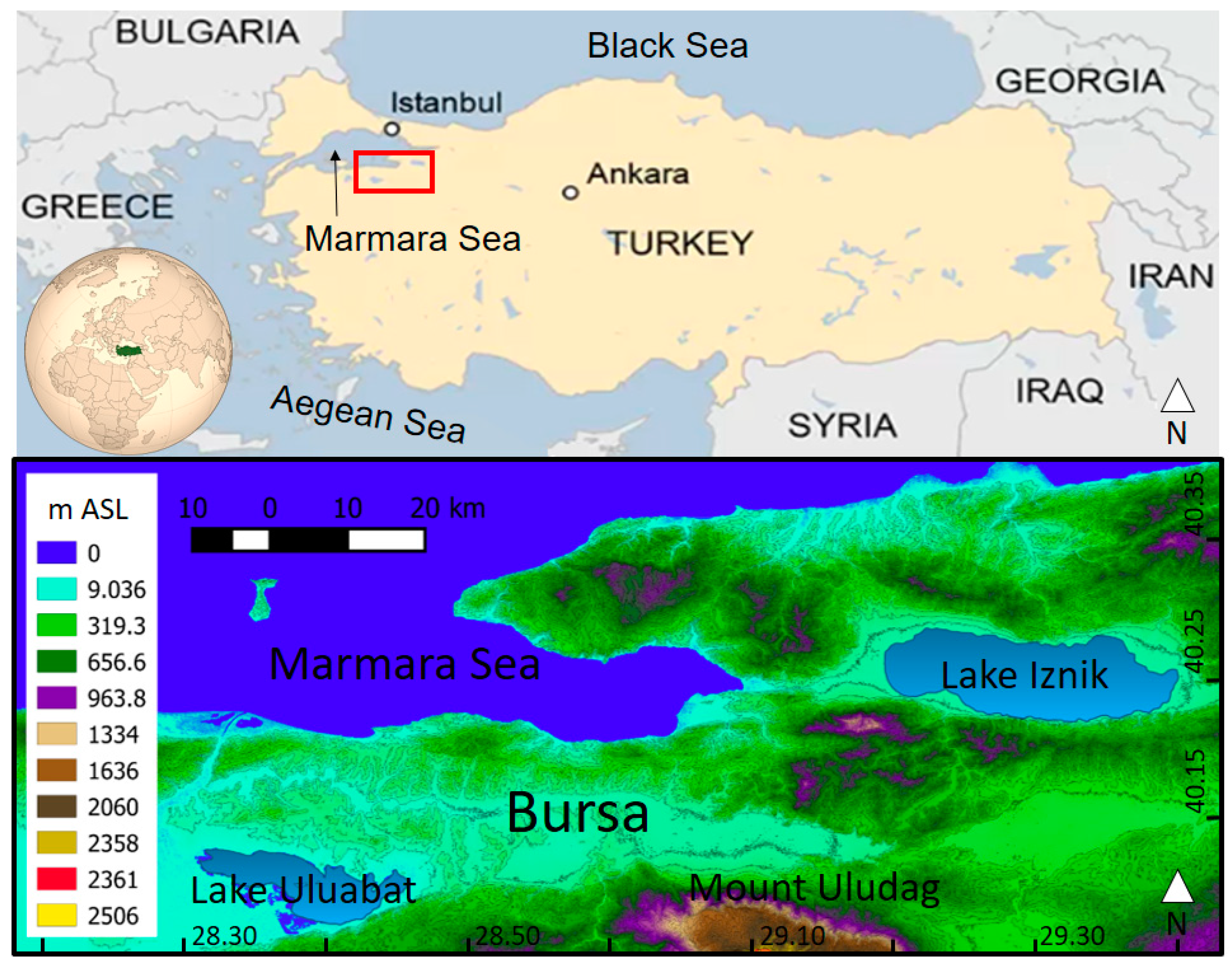
2.1. Study Area
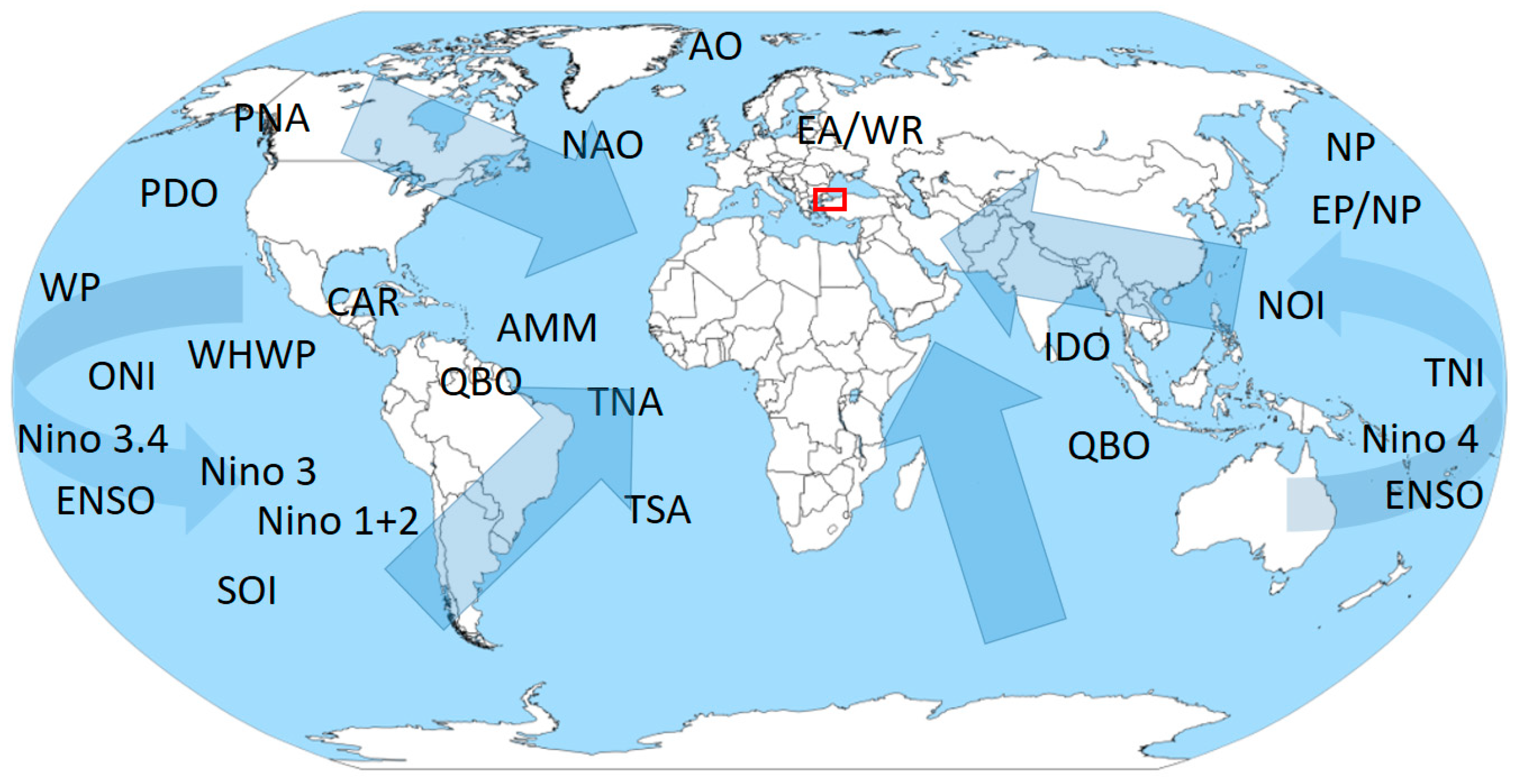
2.2. Data
2.3. Models
2.3.1. Extreme Learning Method (ELM)
2.3.2. Genetic Algorithm (GA)
2.3.3. Invasive Weed Optimization (IWO)
2.3.4. Hybrid ELM-GA and ELM-IWO Models
2.3.5. Performance Evaluation Criteria
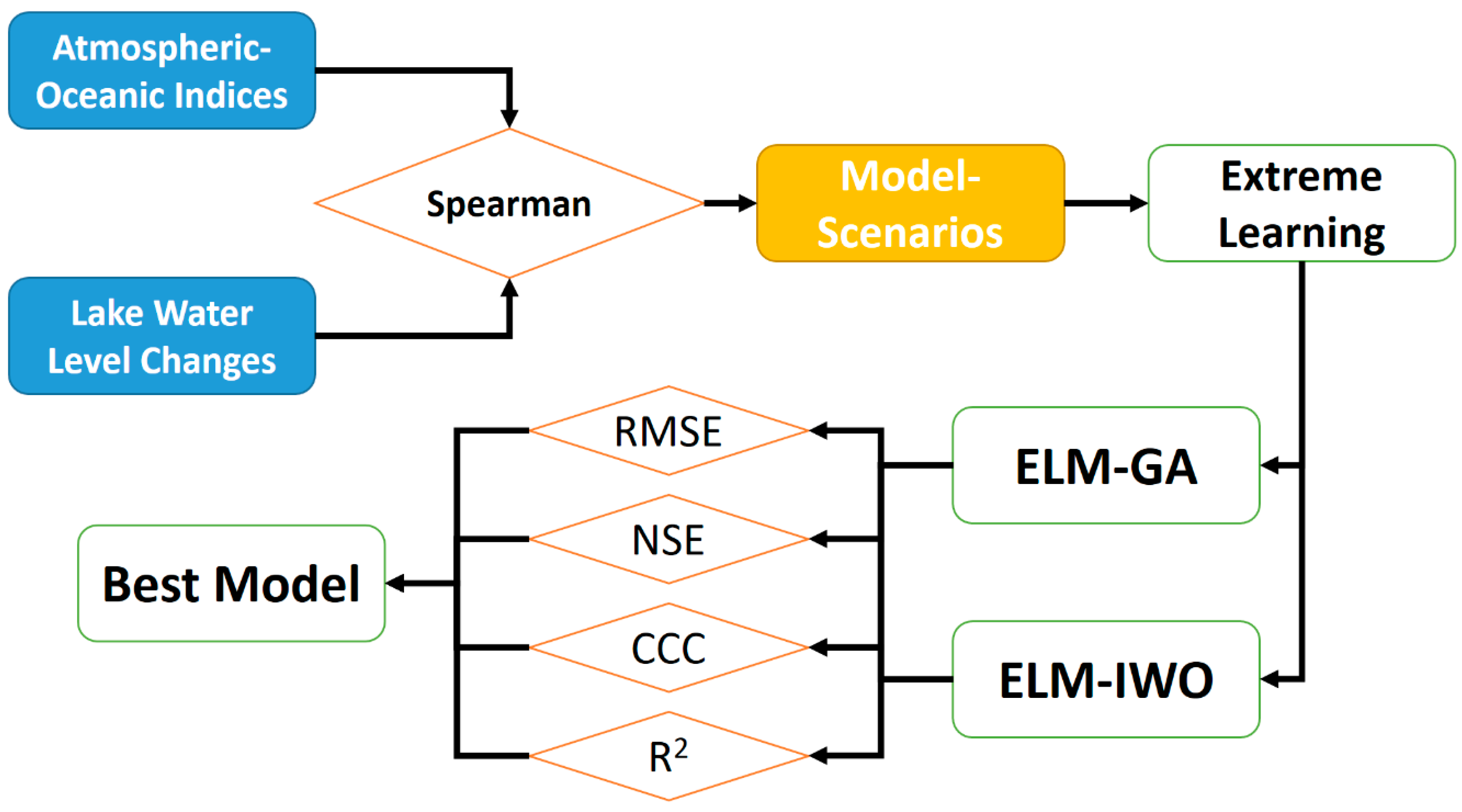
2.3.6. Summarizing the Modeling
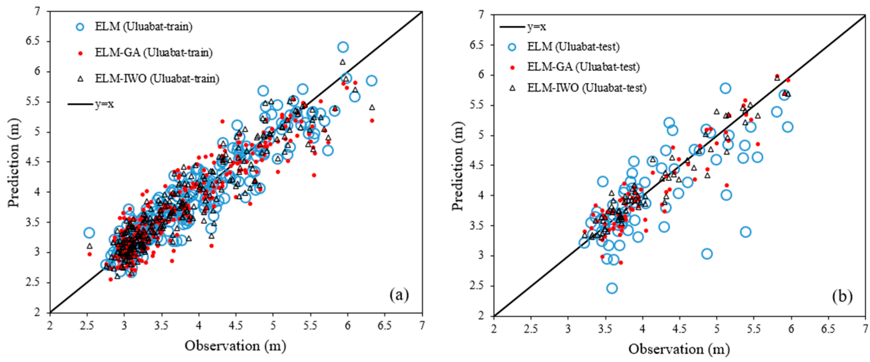
3. Results
4. Discussion
5. Conclusions
Supplementary Materials
Funding
Institutional Review Board Statement
Informed Consent Statement
Data Availability Statement
Acknowledgments
Conflicts of Interest
References
- Xu, N.; Lu, H.; Li, W.; Gong, P. Natural lakes dominate global water storage variability. Sci. Bull. 2024, 69, 1016–1019. [Google Scholar] [CrossRef]
- Vaheddoost, B.; Fathian, F.; Gul, E.; Safari, M.J.S. Studying the Changes in the Hydro-Meteorological Components of Water Budget in Lake Urmia. Water Resour. Res. 2022, 58, e2022WR032030. [Google Scholar] [CrossRef]
- Angel, J.R.; Kunkel, K.E. The response of Great Lakes water levels to future climate scenarios with an emphasis on Lake Michigan-Huron. J. Great Lakes Res. 2010, 36, 51–58. [Google Scholar] [CrossRef]
- Haghighi, A.T.; Kløve, B. A sensitivity analysis of lake water level response to changes in climate and river regimes. Limnologica 2015, 51, 118–130. [Google Scholar] [CrossRef]
- Woolway, R.I.; Kraemer, B.M.; Lenters, J.D.; Merchant, C.J.; O’Reilly, C.M.; Sharma, S. Global lake responses to climate change. Nat. Rev. Earth Environ. 2020, 1, 388–403. [Google Scholar] [CrossRef]
- Bai, B.; Mu, L.; Ma, C.; Chen, G.; Tan, Y. Extreme water level changes in global lakes revealed by altimetry satellites since the 2000s. Int. J. Appl. Earth Obs. Geoinf. 2024, 127, 103694. [Google Scholar] [CrossRef]
- Aminjafari, S.; Brown, I.A.; Frappart, F.; Papa, F.; Blarel, F.; Mayamey, F.V.; Jaramillo, F. Distinctive patterns of water level change in Swedish lakes driven by climate and human regulation. Water Resour. Res. 2024, 60, e2023WR036160. [Google Scholar] [CrossRef]
- Wu, C.; Liu, G.; Cong, L.; Li, X.; Liu, X.; Liu, Y.; Deyan, W.; Zhang, Y.; Bai, D. ENSO-driven hydroclimate changes in central Tibetan Plateau since middle Holocene: Evidence from Zhari Namco’s lake sediments. Quat. Sci. Rev. 2024, 330, 108593. [Google Scholar] [CrossRef]
- Fuentes-Aguilera, P.; Rodríguez-López, L.; Bourrel, L.; Frappart, F. Recovery of Time Series of Water Volume in Lake Ranco (South Chile) through Satellite Altimetry and Its Relationship with Climatic Phenomena. Water 2024, 16, 1997. [Google Scholar] [CrossRef]
- Mologni, C.; Revel, M.; Chaumillon, E.; Malet, E.; Coulombier, T.; Sabatier, P.; Brigode, P.; Herve, G.; Develle, A.L.; Schenini, L.; et al. 50-year seasonal variability in East African droughts and floods recorded in central Afar lake sediments (Ethiopia) and their connections with the El Niño–Southern Oscillation. Clim. Pas. 2024, 20, 1837–1860. [Google Scholar] [CrossRef]
- Shiri, J.; Shamshirband, S.; Kisi, O.; Karimi, S.; Bateni, S.M.; Hosseini Nezhad, S.H.; Hashemi, A. Prediction of water-level in the Urmia Lake using the extreme learning machine approach. Water Resour. Manag. 2016, 30, 5217–5229. [Google Scholar] [CrossRef]
- Zhu, S.; Hrnjica, B.; Ptak, M.; Choiński, A.; Sivakumar, B. Forecasting of water level in multiple temperate lakes using machine learning models. J. Hydrol. 2020, 585, 124819. [Google Scholar] [CrossRef]
- Zhen, L.; Bărbulescu, A. Comparative Analysis of Convolutional Neural Network-Long Short-Term Memory, Sparrow Search Algorithm-Backpropagation Neural Network, and Particle Swarm Optimization-Extreme Learning Machine Models for the Water Discharge of the Buzău River, Romania. Water 2024, 16, 289. [Google Scholar] [CrossRef]
- Sales, A.K.; Gul, E.; Safari, M.J.S.; Ghodrat Gharehbagh, H.; Vaheddoost, B. Urmia lake water depth modeling using extreme learning machine-improved grey wolf optimizer hybrid algorithm. Theor. Appl. Climatol. 2021, 146, 833–849. [Google Scholar] [CrossRef]
- Vaheddoost, B. Spatial analysis of large atmospheric oscillations and annual precipitation in Lake Urmia basin. Eur. Water 2017, 59, 123–129. [Google Scholar]
- Wang, J.; Kessler, J.; Bai, X.; Clites, A.; Lofgren, B.; Assuncao, A.; Bratton, J.; Chu, P.; Leshkevich, G. Decadal variability of Great Lakes ice cover in response to AMO and PDO, 1963–2017. J. Clim. 2018, 31, 7249–7268. [Google Scholar] [CrossRef]
- Komatsu, E.; Fukushima, T.; Harasawa, H. A modeling approach to forecast the effect of long-term climate change on lake water quality. Ecol. Model. 2007, 209, 351366. [Google Scholar] [CrossRef]
- Fathian, F.; Vaheddoost, B. Conceptualization of the indirect link between climate variability and lake water level using conditional heteroscedasticity. Hydrol. Sci. J. 2021, 66, 1907–1923. [Google Scholar] [CrossRef]
- Ozdemir, S.; Yaqub, M.; Yildirim, S.O. A systematic literature review on lake water level prediction models. Environ. Model. Softw. 2023, 163, 105684. [Google Scholar] [CrossRef]
- Kottek, M.; Grieser, J.; Beck, C.; Rudolf, B.; Rubel, F. World Map of the Köppen-Geiger climate classification updated. Meteorol. Z. 2006, 15, 259–263. [Google Scholar] [CrossRef]
- National Oceanic and Atmospheric Administration (NOAA). Climate Indices: Monthly Atmospheric and Ocean Time Series. Available online: https://psl.noaa.gov/data/climateindices/list/ (accessed on 1 August 2024).
- Huang, G.B.; Zhu, Q.Y.; Siew, C.K. Extreme learning machine: A new learning scheme of feedforward neural networks. In Proceedings of the IEEE International Joint Conference on Neural Networks (IEEE Cat. No. 04CH37541), Budapest, Hungary, 25–29 July 2004; Volume 2, pp. 985–990. Available online: https://ieeexplore.ieee.org/xpl/conhome/9486/proceeding (accessed on 1 August 2024).
- Safari, M.J.S.; Ebtehaj, I.; Bonakdari, H.; Eshaghi, M.S. Sediment transport modeling in rigid boundary open channels using generalize structure of group method of data handling. J. Hydrol. 2019, 577, 123951. [Google Scholar] [CrossRef]
- Holland, J.H. Adaptation in Natural and Artificial Systems: An Introductory Analysis with Applications to Biology, Control, and Artificial Intelligence; MIT Press: Cambridge, MA, USA, 1992; Available online: https://ieeexplore.ieee.org/book/6267401 (accessed on 1 August 2024).
- Mehrabian, A.R.; Lucas, C. A novel numerical optimization algorithm inspired from weed colonization. Ecol. Inform. 2006, 1, 355–366. [Google Scholar] [CrossRef]
- Safari, M.J.S.; Mohammadi, B.; Kargar, K. Invasive weed optimization-based adaptive neuro-fuzzy inference system hybrid model for sediment transport with a bed deposit. J. Clean. Prod. 2020, 276, 124267. [Google Scholar] [CrossRef]
- Vaheddoost, B.; Guan, Y.; Mohammadi, B. Application of hybrid ANN-whale optimization model in evaluation of the field capacity and the permanent wilting point of the soils. Environ. Sci. Pollut. Res. 2020, 27, 13131–13141. [Google Scholar] [CrossRef]
- Gul, E.; Staiou, E.; Safari, M.J.S.; Vaheddoost, B. Enhancing Meteorological Drought Modeling Accuracy Using Hybrid Boost Regression Models: A Case Study from the Aegean Region, Türkiye. Sustainability 2023, 15, 11568. [Google Scholar] [CrossRef]
- Zar, J.H. Spearman Rank Correlation. In Biostatistical Analysis, 5th ed.; Pearson Prentice-Hall: Hoboken, NJ, USA, 2005; pp. 388–394. [Google Scholar]
- Ghanbari, R.N.; Bravo, H.R. Coherence between atmospheric teleconnections, Great Lakes water levels, and regional climate. Adv. Water. Resour. 2008, 31, 1284–1298. [Google Scholar] [CrossRef]
- Guo, J.; Sun, J.; Chang, X.; Guo, S.; Liu, X. Correlation analysis of NINO3. 4 SST and inland lake level variations monitored with satellite altimetry: Case studies of lakes Hongze, Khanka, La-ang, Ulungur, Issyk-kul and Baikal. TAO Terr. Atmos. Ocean. Sci. 2011, 22, 2. [Google Scholar] [CrossRef]


| N. | LSAOO | Extension | About |
|---|---|---|---|
| 1 | AMM | Atlantic Meridional Mode | Cross-equatorial meridional difference in SST anomaly in the tropical Atlantic |
| 2 | AO | Arctic Oscillation | Back-and-forth shifting of AP between the Arctic and the mid-latitudes of the North Pacific and North Atlantic |
| 3 | CAR | Caribbean SST Index | SST anomalies averaged over the Caribbean |
| 4 | EA/WR | Eastern Asia/Western Russia | Large-scale anomalies over the Caspian Sea toward western Europe |
| 5 | ENSO | Multivariate El Niño–Southern Oscillation Index | Empirical orthogonal function of SLP, SST, zonal, and meridional components of the surface wind and outgoing longwave radiation over the tropical Pacific basin (30° S–30° N and 100° E–70° W) |
| 6 | EP/NP | East Pacific/North Pacific Oscillation | Spring–Summer–Fall pattern focused on three anomaly centers |
| 7 | IDO | Indian Dipole Oscillation | Anomalous SST gradient between the western equatorial Indian Ocean (50° E–70° E and 10° S–10° N) and the south eastern equatorial Indian Ocean (90° E–110° E and 10° S–0° N) |
| 8 | NAO | North Atlantic Oscillations | Difference in normalized pressure between Iceland and the Azores |
| 9 | Niño 1 + 2 | Extreme Eastern Tropical Pacific SST | The average SST between 0°~10° S and 90°~80° W |
| 10 | Niño 3 | Eastern Tropical Pacific SST | The average SST between 5° S~5° N and 150°~90° W |
| 11 | Niño 3.4 | East Central Tropical Pacific SST | The average SST between 5° S~5° N and 170°~120° W |
| 12 | Niño 4 | Central Tropical Pacific SST | The average SST between 5° S~5° N and 160° E~150° W |
| 13 | NOI | Northern Oscillation Index | The difference in SLP between Darwin in Australia and the North Pacific High |
| 14 | NP | North Pacific pattern | Sea level differences between 30°~65° N and 160° E~145 ° W |
| 15 | ONI | Oceanic Niño Index | 3-month averaged SST in the east-central tropical Pacific (120°–170° W) near the International Dateline |
| 16 | PDO | Pacific Decadal Oscillation | Temporal covariance matrix of SST in the Pacific |
| 17 | PNA | Pacific North American index | Anomalies in the geopotential height fields of 700 or 500 mb over the western and eastern US |
| 18 | QBO | Quasi-Biennial Oscillation | A quasiperiodic oscillation between easterlies and westerlies of the equatorial zonal wind in the tropical stratosphere |
| 19 | SOI | Southern Oscillation Index | The difference between normalized pressure in Tahiti and Darwin |
| 20 | TNA | Tropical Northern Atlantic index | SST between 15°~57.5° W and 5.5°~23.5 ° N |
| 21 | TNI | Trans-Niño Index | The difference between normalized anomalies of SST between Niño 1 + 2 and Niño 4 |
| 22 | TSA | Tropical Southern Atlantic index | SST between 30° W~10° E and 20° S~0° |
| 23 | WHWP | Western Hemisphere Warm Pool | The SST (when it is hotter than 28.5 °C) in the eastern North Pacific and Atlantic oceans |
| 24 | WP | Western Pacific Index | Low-frequency oscillations over the North Pacific |
| GA | IWO | ||
|---|---|---|---|
| Population size | 50 | Population size | 50 |
| Number of generations | 100 | Number of generations | 100 |
| Reproduction method | Crossover and mutation | Reproduction method | Based on fitness |
| Crossover fraction | 0.8 | Number of seeds | 1–5 |
| Mutation function | mutationadaptfeasible | Sigma | 0.001–0.1 |
| Model | Stage | RMSE | NSE | CCC | R2 | AIC |
|---|---|---|---|---|---|---|
| ELM | Training | 0.064 | 0.969 | 0.984 | 0.969 | 16.033 |
| Testing | 0.208 | 0.634 | 0.822 | 0.692 | 16.342 | |
| ELM-GA | Training | 0.092 | 0.935 | 0.966 | 0.935 | 16.069 |
| Testing | 0.092 | 0.929 | 0.964 | 0.928 | 16.071 | |
| ELM-IWO | Training | 0.067 | 0.966 | 0.983 | 0.965 | 16.036 |
| Testing | 0.096 | 0.921 | 0.960 | 0.925 | 16.076 |
| Model | Stage | RMSE | NSE | CCC | R2 | AIC |
|---|---|---|---|---|---|---|
| ELM | Training | 0.276 | 0.884 | 0.939 | 0.884 | 29.091 |
| Testing | 0.533 | 0.443 | 0.723 | 0.539 | 32.159 | |
| ELM-GA | Training | 0.325 | 0.839 | 0.913 | 0.873 | 29.514 |
| Testing | 0.289 | 0.836 | 0.918 | 0.839 | 29.276 | |
| ELM-IWO | Training | 0.283 | 0.878 | 0.935 | 0.878 | 29.149 |
| Testing | 0.194 | 0.926 | 0.962 | 0.927 | 28.582 |
Disclaimer/Publisher’s Note: The statements, opinions and data contained in all publications are solely those of the individual author(s) and contributor(s) and not of MDPI and/or the editor(s). MDPI and/or the editor(s) disclaim responsibility for any injury to people or property resulting from any ideas, methods, instructions or products referred to in the content. |
© 2024 by the author. Licensee MDPI, Basel, Switzerland. This article is an open access article distributed under the terms and conditions of the Creative Commons Attribution (CC BY) license (https://creativecommons.org/licenses/by/4.0/).
Share and Cite
Can, M. Invasive-Weed-Optimization-Based Extreme Learning Machine for Prediction of Lake Water Level Using Major Atmospheric–Oceanic Climate Scenarios. Sustainability 2024, 16, 7825. https://doi.org/10.3390/su16177825
Can M. Invasive-Weed-Optimization-Based Extreme Learning Machine for Prediction of Lake Water Level Using Major Atmospheric–Oceanic Climate Scenarios. Sustainability. 2024; 16(17):7825. https://doi.org/10.3390/su16177825
Chicago/Turabian StyleCan, Murat. 2024. "Invasive-Weed-Optimization-Based Extreme Learning Machine for Prediction of Lake Water Level Using Major Atmospheric–Oceanic Climate Scenarios" Sustainability 16, no. 17: 7825. https://doi.org/10.3390/su16177825
APA StyleCan, M. (2024). Invasive-Weed-Optimization-Based Extreme Learning Machine for Prediction of Lake Water Level Using Major Atmospheric–Oceanic Climate Scenarios. Sustainability, 16(17), 7825. https://doi.org/10.3390/su16177825