Travel Time Estimation for Urban Arterials Based on the Multi-Source Data

Abstract

Accurate traffic information, such as travel time, becomes more important since it could help provide more efficient traffic management strategies. This paper presents a method for estimating the travel time of segments on urban arterials by leveraging multi-source data from loop detectors and probe vehicles. Travel time is defined into three distinct sections based on floating car trajectories, i.e., accelerating, constant speed, and decelerating. Considering the traffic flow characteristics, different methods are developed using various data for each section. The proposed methodology is validated using field data collected in Shanghai, China. The results validated the proposed method with absolute percentage errors (APEs) of approximately 5% in constrained traffic flow conditions and 10–20% in less constrained traffic flow. The results also show that the proposed method has better performance than the method with loop detector data and another data fusion model. It is expected that the proposed method could help improve traffic management efficiency, such as traffic signal control, by providing more accurate travel time information.

1. Introduction

In the realm of urban transportation, the estimation of travel time emerges as a pivotal metric for assessing the efficacy of arterial roads. Accurate and reliable travel time estimations provide travelers with data on the optimal route selection based on their individual needs, preferences, and the current state of the transportation network [1]. It grants travelers the ability to minimize travel time and enhance travel efficiency.

The accurate estimation of travel time not only enhances the quality of life by enabling individuals but also plays a critical role in the strategic planning by city planners and policymakers. With knowledge of travel times across various routes, better traffic management and infrastructure planning can be achieved. This information can inform decisions regarding investments in new roads, public transportation systems, or traffic signal technologies, all aimed at reducing congestion and enhancing mobility. Thus, accurate travel time estimation is essential for sustainable urban transportation systems. Given its significance, numerous techniques have been developed to collect travel time information.

Travel time information can be categorized into two distinct categories, i.e., path travel time and link travel time information [2]. In the context of path travel time, three predominant methodologies are utilized. Initially, the estimation of path travel time is achieved through direct measurement via mobile sensors, such as Floating Car Data (FCD) and Global Positioning System (GPS) data [3,4]. Nonetheless, the precision is frequently compromised by factors such as low sampling rates and the presence of noise interference. Subsequently, the path travel time is deduced as the cumulative link travel time of the constituent links [5]. Link travel time is usually modeled using data from stationary sensors. However, intersection delays are often overlooked [6]. Lastly, an enhanced model, integrating data from both stationary and mobile sensors, is employed to yield more dependable outcomes [7,8].

In terms of the link travel time, current data used to estimate link travel time are from stationary and/or mobile sensors [9]. When from stationary sensors, two primary methods are commonly employed. One approach involves the development of estimation models based on traffic flow data obtained from vehicle passage detections using stationary sensors like loop detectors [10]. Alternatively, travel time data can be obtained by vehicle identification at various points using stationary sensors such as Automatic Vehicle Identification (AVI), Electronic Toll Collection (ETC), Radio Frequency Identification (RFID), or other technologies [11,12,13]. Mobile sensors, on the other hand, can track vehicle data, which can then be transmitted to provide travel time information. This includes Floating Car Data (FCD), Bluetooth technology, and even mobile phone probes [14,15,16,17]. For example, Sun et al. used large-scale, incomplete taxi trip records to estimate the mean travel time for special link [18]. The taxi trip records were from NYC taxi and Chengdu DiDi, which contained only the end-point information of each trip. The link travel time was estimated by the non-negative least-squares estimation after determining the inferred path based on the path recovery. The experimental results demonstrate that their proposed model greatly improved the accuracy of travel time estimation.

A significant body of literature on travel time estimation has emerged regarding the above techniques. Most travel time estimation models in the literature have been developed for freeways [19]. Progress in travel time estimation on urban arterials, however, has lagged that of freeways. This is due, in part, to challenges associated with improving estimation efficiency and accuracy given the measurement range and precision of data from a single data source. Furthermore, travel time on arterial networks is influenced not only by traffic flow, link capacity, and speed limits but also by factors such as signal timing and conflicting traffic.

To overcome limitations imposed by data sources, data fusion techniques have been applied to link travel time estimations. By fusing multiple data sources, data fusion can enhance the understanding of the observed traffic situation by reducing uncertainty associated with individual sources [20,21].

In the realm of travel time estimation, two primary fusion algorithms have emerged. The initial type of algorithm first calculates travel time for individual data sources independently, then integrates these outcomes to achieve a final estimation. Alternatively, the second type of algorithm simultaneously incorporates data from multiple sources to generate an aggregate estimate. Within the context of the first type of fusion algorithm, techniques such as the weighted average method, Dempster–Shafer theory, Bayesian theory, fuzzy theory, and others are employed to combine travel time estimations [22]. Choi and Chung developed an algorithm and protocol for integrating detector and GPS Floating Car Data to establish a representative link travel time [23]. This involved techniques like voting technique, fuzzy regression, and Bayesian pooling method. Evaluations revealed that the combined link travel time outperformed the simple arithmetic mean approach. Li and Yang introduced a data fusion model derived from the average link travel time model, which was based on the population of vehicles [24]. This model effectively combined loop detectors and Floating Car Data. Simulations on an urban arterial road with five intersections and four links showed that the data fusion model surpassed the traditional floating car method in terms of results.

For the second type of fusion algorithm, methods like neural networks, traffic theory, and others are employed to combine data from diverse sources. Zou and Zhu proposed a fusion model based on a BP neural network that utilized data from floating cars and loop detectors [25]. This model was developed, tested, and validated using transportation data from Guangzhou City, indicating its validity. Bhaskar et al. integrated real-time cumulative plots, probe vehicles, and historical cumulative plots to propose a real-time estimation of exit movement-specific average travel time on urban routes. The methodology was evaluated through simulations [26].

Traffic theory-based models rely on concepts like flow conservation, propagation principles, kinematic wave theory, traffic propagation formulas, cumulative plots, and other traffic flow theories [27,28,29]. These models utilize intricate and realistic relationships to capture the dynamic nature of traffic flow. However, traffic theory-based models are not widely implemented when data come from diverse sources, since finding models that accept inputs from multiple sensors can be challenging [30].

In summary, previous studies have presented effective methods for travel time estimation. Nonetheless, most have concentrated on freeways. In recent years, more attention has been paid to arterial networks, though results have not always been satisfactory. Additionally, these studies have not fully leveraged the potential of applying travel time estimation across entire networks.

The primary objective of this paper is to develop and validate a sophisticated method for estimating travel time on urban arterials by dividing the link into three sections, i.e., accelerating, constant-speed, and decelerating sections. The method accounts for the specific traffic flow characteristics of urban arterials, such as signal timing and traffic congestion, which are crucial for modeling the interrupted flow. In the constant-speed section, an enhanced BPR function is used to calculate the travel time. An improved shockwave theory is used in the decelerating section to capture the characteristics due to the interrupted flow. This developed methodology aims to be robust in urban complexities, including influences like entrance/exit traffic and detector counting errors, for real-time applications. It is fundamental to developing sustainable urban transportation systems.

The paper is organized as follows: Section 2 outlines the assumptions and terminologies used in this paper. Section 3 introduces the proposed methodology. Section 4 evaluates the methodology using data from Shanghai. Finally, Section 5 provides conclusions and offers further discussion.

2. Preliminaries

To facilitate the development of formulas for estimating travel time, this section defines several key terminologies. It also presents several assumptions about driving behavior along arterial links, as well as an introduction of the Bureau of Public Roads (BPR) function and the queue formation and discharge process at signalized intersections.

2.1. Terminology Definitions

Link: A combination of an intersection and the downstream road linked to it (Figure 1).

Travel time of the link: The interval of time during which a vehicle travels from the stop line of one intersection to the stop line of the adjacent intersection.

2.2. Assumptions

To facilitate the estimation of travel time, the following assumptions are made:

Roadway Geometry: The geometry of the intersection, including the length of the road and the configuration of lanes, is known.

Signal Timing: The signal timing is known and can operate on either fixed or actuated cycles.

Stationary Sensor Data: Loop detectors need to be installed right behind the stop line to detect passing vehicles and their speeds.

Mobile Sensor Data: In this study, probe vehicles serve as sources of mobile sensor data. Probe data are collected at short intervals (e.g., one second) to determine the spatial and temporal coordinates of the probe vehicles.

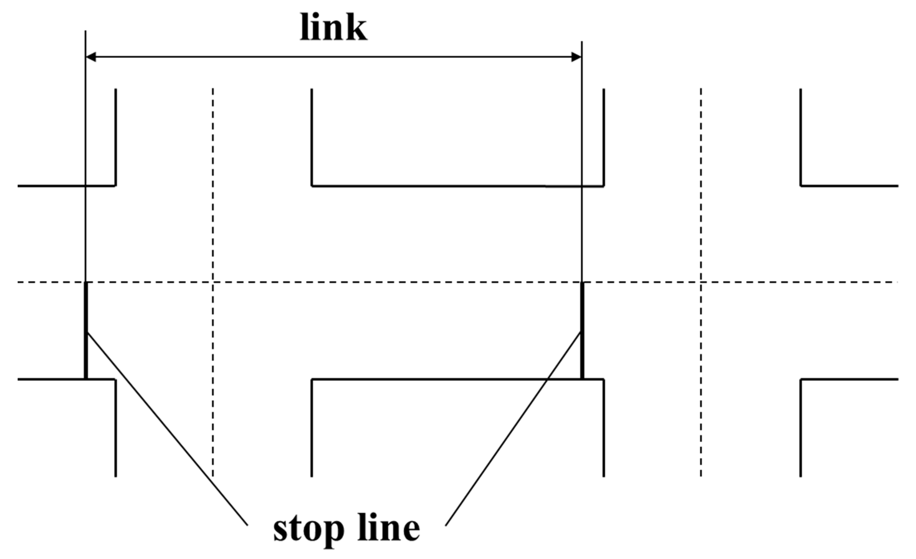
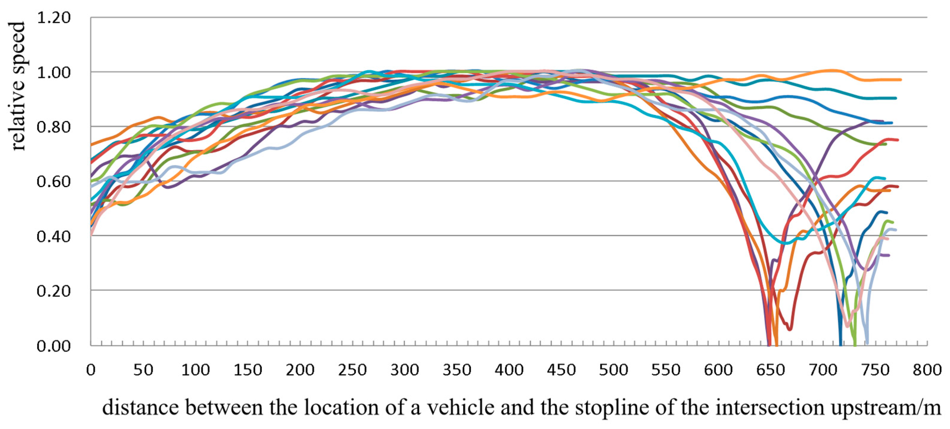
2.3. Driving Behavior along an Arterial Link

The travel time along arterial roads can be divided into two distinct components, i.e., the time required to traverse the links between traffic signal influence areas and the time to traverse the signalized intersection itself [31]. According to the theory, a vehicle accelerates after passing the stop line of the upstream intersection until it reaches a target speed. The acceleration process could be affected by driver habits, traffic conditions, and other factors. The vehicle may pass the stop line of the downstream intersection at a constant speed (Figure 2 ①), or may be influenced by signal control after traveling at a relatively constant speed. Under signal control, the vehicle may experience a stop (Figure 2 ③), or deceleration (Figure 2 ②).

Previous studies pointed out that the estimation of travel time along a link can be divided into three sections, i.e., the accelerating section, the constant-speed section, and the decelerating section (Figure 2) [32].

The travel time can be calculated by the following equation:

$$TT=T_1+T_2+T_3$$

(1)

where $TT$ denotes the travel time of the link; $T_1$ is the travel time of accelerating section; $T_2$ is the travel time of constant-speed section; and $T_3$ is the travel time of decelerating section.

2.4. BPR Function

Numerous volume-delay functions have been proposed and implemented in practice in the past. Among the most widely utilized volume-delay functions is the BPR function, which is defined in Equation (2) [33]. The BPR function is the most widely used volume-delay function for analyzing the relationship between traffic volume and delays in the link level. The BPR function is computationally efficient and has good mathematical properties with only two parameters. All these advantages make it well-suited for practical traffic planning and management [34].

$$v={\displaystyle \frac{V_f}{1+\gamma {\left(\frac{q}{c}\right)}^{\beta }}}$$

(2)

where v denotes the speed of the link; $V_f$ is the speed of free flow; q is traffic flow; c is the capacity of the link; and $\gamma$ and $\beta$ are parameters.

However, it should be noted that the BPR function was originally developed based on data from uncongested highways. When applied to arterial networks, the BPR function may produce results with significant deviations. Furthermore, under congestion conditions, the BPR function may not fully capture all the features as proposed by Blunden [35].

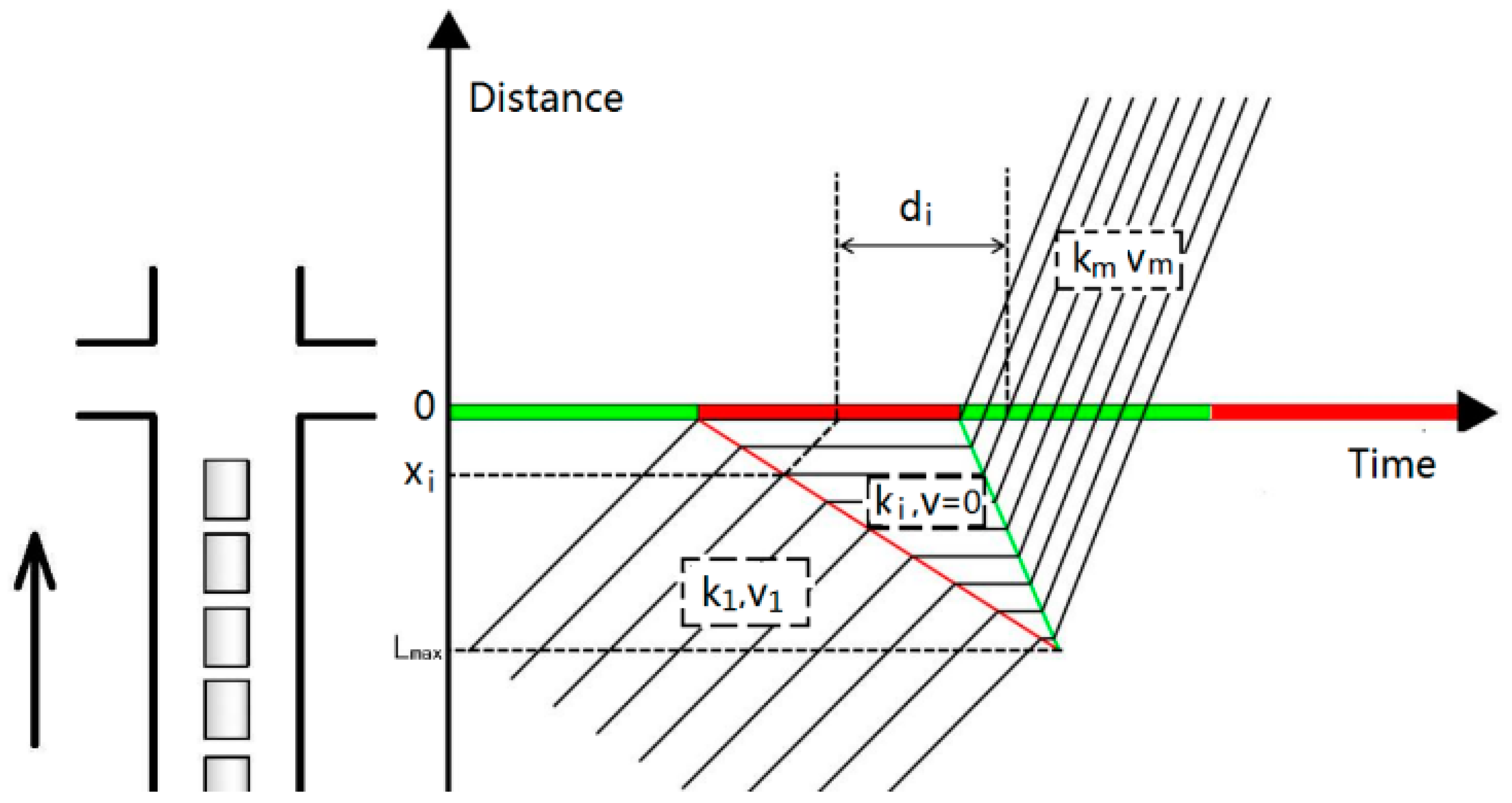
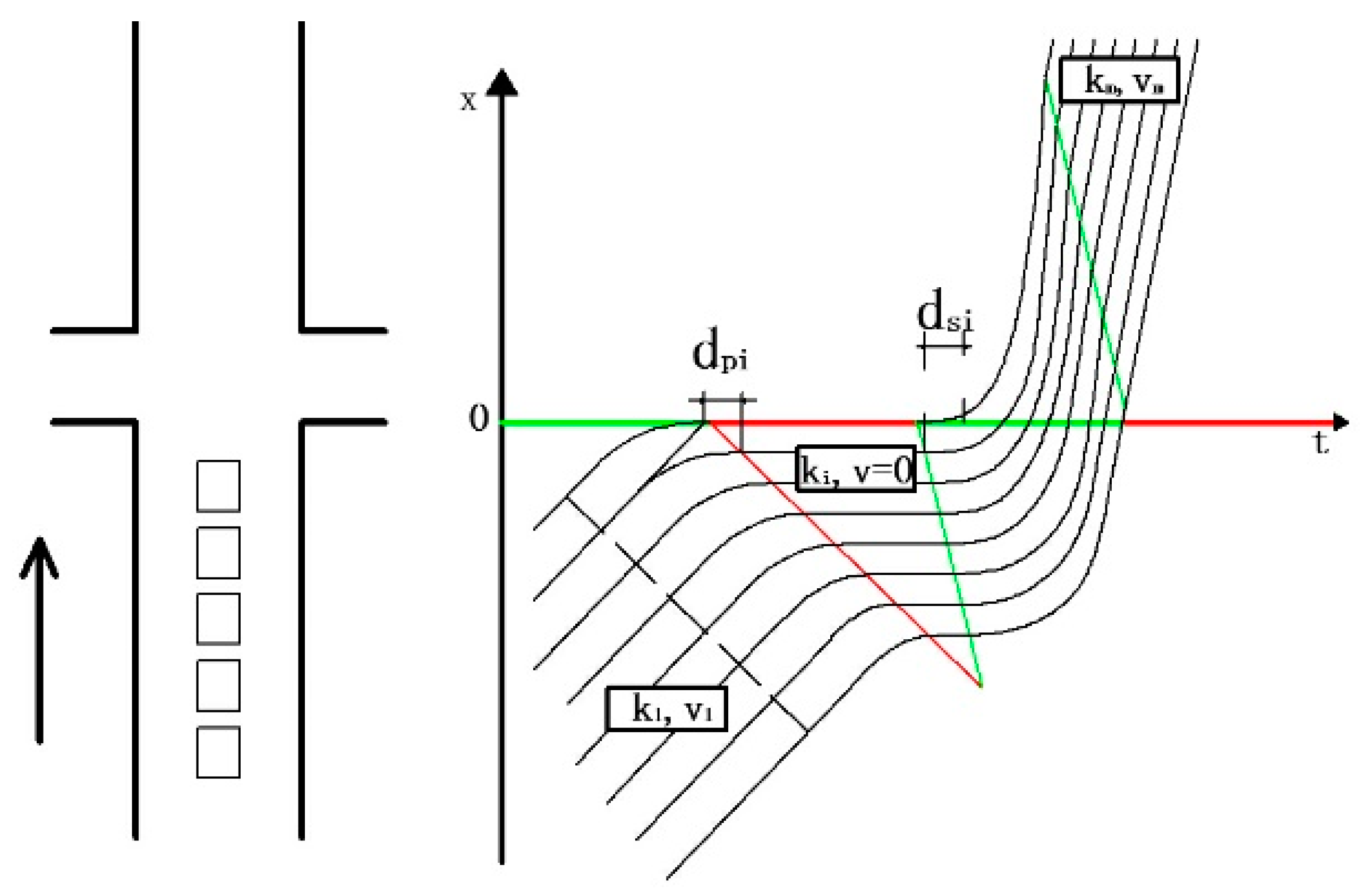
2.5. Queue Forming and Discharging Process

When different traffic flow interacts, a shockwave is formed. The speed of the shockwave can be determined by Equation (3) [36].

$$u_w={\displaystyle \frac{\Delta q}{\Delta k}}={\displaystyle \frac{q_2-q_1}{k_2-k_1}}$$

(3)

where $u_w$ is the speed of a shockwave; $q_1$ and $k_1$ are the flow and density of the upstream region, respectively; and $q_2$ and $k_2$ are the flow and density of the downstream region, respectively.

As shown in Figure 3, the red line represents the queuing shockwave, and the green line is the discharge shockwave. The starting and parking wave speeds are the gradients of the red line and green line [37]. According to Equation (3), the wave speed can be calculated as Equations (4) and (5) [38].

$$u_{ws}={\displaystyle \frac{k_2{v}_2}{k_2-k_j}}$$

(4)

$$u_{wp}={\displaystyle \frac{k_1{v}_1}{k_1-k_j}}$$

(5)

where u_ws is the starting wave speed; u_wp is the parking wave speed; k₂ and v₂ are the density and speed of saturation traffic flow; k₁ and v₁ are the density and speed of average arrival flow; and k_j is the jammed density.

Based on the shockwave theory, the process of queue forming and discharging at a signalized intersection can be approximated (Figure 3).

According to Figure 3, the graphical method is used to calculate approach delay, as Equation (6) shows.

$$d_i=r+x_i\left({\displaystyle \frac{1}{v_m}}+{\displaystyle \frac{1}{u_{ws}}}-{\displaystyle \frac{1}{v_1}}-{\displaystyle \frac{1}{u_{wp}}}\right)$$

(6)

where d_i denotes the approach delay of the i-th vehicle; r is the red phase; x_i is the distance between where the i-th vehicle stops in the queue and the stop line of intersection downstream; and v_m is the saturation speed.

Based on the shockwave theory and Equations (3)–(6), the average approach delay can be calculated by using Equation (7).

$$d_{ap}={\displaystyle \frac{\sum _i^N{d}_i}{N}}=r·(1+{\displaystyle \frac{1}{2}}·{\displaystyle \frac{k_j\left(q_1-s\right)}{s\left(k_j-k_1\right)-q_1\left(k_j-k_m\right)}})$$

(7)

where $k_m$ is the saturation density; s is the saturation traffic rate; and $q_1$ is the volume of average arrival flow.

However, according to the definition of approach delay, the acceleration and deceleration of vehicles ignored in shockwave theory are crucial. An improved algorithm will be developed in next section.

3. Methodology

In the proposed method, the estimation of travel time is divided into two steps. Initially, data from probe vehicles and loop detectors are integrated to estimate the travel time for each section of the link. Subsequently, the travel time for the arterial link is computed by summing the travel times of each section.

3.1. Accelerating Section

The travel time estimation for the accelerating section assumes a functional relationship between speed and the distance from the point used to calculate speed to the stop line of the upstream intersection, as described in Equation (8).

$$v=a_1{x}^2+a_{2}x+a_3$$

(8)

where $\mathrm{v}$ notes the average speed; $a_1$, $a_2$, and $a_3$ are the parameters; and $x$ is the distance between the point used to calculate the speed and stop line of intersection upstream.

The boundary conditions include the following: ① v = $V_{0,k}$ for x = 0; ② v = $V_k\prime$ for x = $L_{1,k }$, namely the length of the accelerating section of link k; and ③ ${\displaystyle \frac{dv}{dt}}$ = 0 for v = $V_k\prime$. Take the derivative of Equation (8) with respect to time to calculate ${\displaystyle \frac{dv}{dt}}$ as Equation (9) shows.

$${\displaystyle \frac{dv}{dt}}=v\sqrt{{a_2}^2-{4a}_1(a_3-v)}$$

(9)

The parameters are calculated as Equation (10) shows.

$$\left\{\begin{array}{cc}\hfill a_1& ={\displaystyle \frac{\left(V_{0,k}-{V_k}^{\prime }\right)}{{L_{1,k}}^2}}\hfill \\ \hfill a_2& =-{\displaystyle \frac{2\left(V_{0,k}-{V_k}^{\prime }\right)}{L_{1,k}}}\hfill \\ \hfill a_3& =V_{0,k}\hfill \end{array}\right.$$

(10)

where $V_{0,k}$ denotes the mean speed of pulling out of the stopline of intersection upstream of link $i$ and gained by loop detectors; ${V_k}^{\prime }$ is the mean speed of vehicles traveling through the constant-speed section of link $k$; and $L_{1,k }$ is the length of accelerating section of link $k$.

Taking the values of parameters in Equations (9) and (10), Equation (11) calculates the travel time of the accelerating section.

$${\displaystyle \frac{dt}{dv}}={\displaystyle \frac{L_{1,k }}{2\sqrt{{V_k}^{\prime }-V_{0,k}}}}·{\displaystyle \frac{1}{v\sqrt{{V_k}^{\prime }-v}}}$$

(11)

Compute the integral for Equation (11) to obtain Equation (12).

$$t=-{\displaystyle \frac{L_{1,k }arctanh\left(\frac{\sqrt{{V_k}^{\prime }-v}}{\sqrt{{V_k}^{\prime }}}\right)}{\sqrt{{V_k}^{\prime }-V_{0,k}}\sqrt{{V_k}^{\prime }}}}+g$$

(12)

where g denotes a parameter $arctanh\left(x\right)={\displaystyle \frac{1}{2}}\mathit{ln}\left({\displaystyle \frac{1+x}{1-x}}\right),x\in (-\mathrm{1,1})$.

Taking boundary condition into consideration, g is calculated by Equation (13).

$$g={\displaystyle \frac{L_{1,k}arctanh\left(\frac{\sqrt{{V_k}^{\prime }-V_{0,k}}}{\sqrt{{V_k}^{\prime }}}\right)}{\sqrt{{V_k}^{\prime }-V_{0,k}}\sqrt{{V_k}^{\prime }}}}$$

(13)

And the travel time of the accelerating section is estimated by Equation (14).

$$T_1={\displaystyle \frac{L_{1}arctanh\left(\frac{\sqrt{{V_k}^{\prime }-V_{0,k}}}{\sqrt{{V_k}^{\prime }}}\right)}{\sqrt{{V_k}^{\prime }-V_{0,k}}\sqrt{{V_k}^{\prime }}}}$$

(14)

3.2. Constant-Speed Section

In the segment characterized by a constant speed, we postulated that the traffic flow remains static. While the BPR function is typically suited for uninterrupted traffic flow, it can be adapted for application in this segment through appropriate modifications. To enhance the precision of estimating average travel time on urban arterial roads, we proposed a method to modify BPR functions. These modifications are derived through data fitting using highway data from China, as expressed in Equation (15) and further detailed in reference [39].

$$\left\{\begin{array}{l}v={\displaystyle \frac{b_1{V}_f}{1+{\left(\frac{q}{c}\right)}^{\beta }}} \\ \beta =b_2+b_3{\left({\displaystyle \frac{q}{c}}\right)}^3\end{array}\right.$$

(15)

where b₁, b₂, and b₃ are parameters.

Considering the limitations imposed by speed and vehicle types within arterial networks, b₁ exerts minimal influence. Furthermore, various traffic conditions may exhibit identical traffic volumes according to the fundamental diagram of traffic flow. This aspect becomes especially crucial when estimating the speeds on arterial networks. Therefore, we introduced an enhanced BPR model specifically designed to estimate the travel time within constant-speed sections. This improved model is formulated and presented in Equation (16).

$$\left\{\begin{array}{l}{V_k}^{\prime }={\displaystyle \frac{V_{max,k}}{1+\gamma {\left(\raisebox{1ex}{$q$}\!\left/ \!\raisebox{-1ex}{$c$}\right.\right)}^{\beta }}} \\ \beta =b_1+b_2{\left({\displaystyle \raisebox{1ex}{$q$}\!\left/ \!\raisebox{-1ex}{$c$}\right.}\right)}^3\end{array}\right.$$

(16)

where $V_{max,k}$ denotes the maximum speed of constant-speed section and gained by FCD. To simplify the calculation, $\gamma$ is equal to 1 in the case study. And based on validation of Wang [39], $b_1$ is equal to 1.88 and $b_2$ is equal to 7.0.

And the travel time of a constant-speed section is estimated by Equation (17).

$$T_2={\displaystyle \frac{L_{2,k}}{{V_k}^{\prime }}}$$

(17)

where $L_{2,k}$ denotes the length of constant-speed section of link $k$.

3.3. Decelerating Section

In the section characterized by deceleration, the travel time is predominantly influenced by the signalized intersection located downstream. In alignment with the definition of a link, this section incorporates the concept of approach delay for estimating travel time. Approach delay, as defined in reference [40], refers to the delay incurred upstream of an intersection and encompasses deceleration and stopped delays, along with the acceleration delay prior to the intersection.

Acceleration and deceleration are often overlooked in traditional shockwave theory. Given the importance of acceleration and deceleration in calculating approach delay, this article introduces an enhanced shockwave theory framework. This improved methodology serves as a more accurate means of calculating approach delay (Figure 4).

$d_{pi}$ denotes the deceleration delay of the vehicle $i$, while $d_{si}$ denotes the accelerating delay of the vehicle $i$.

The deceleration rate is assumed to be constant. And according to kinetics, the deceleration delay can be calculated by Equation (18).

$$\left\{\begin{array}{c}{d}_{pi}=t_{p2}-t_{p1} \\ {0.5a}_p{t}_{p2}^2={V_k}^{\prime }{t}_{p1}\\ {V_k}^{\prime }=a_p{t}_{p2} \end{array}\right.$$

(18)

where $d_{pi}$ denotes deceleration delay of the i-th vehicle; $a_p$ is the deceleration rate;$t_{p2}$ is the time to decelerate; and $t_{p1}$ is the time to traverse the deceleration distance at $v_k’$. The deceleration delay of the vehicle $i$ can be calculated as Equation (19).

$$d_{pi}={\displaystyle \frac{{V_k}^{\prime }}{2a_p}}$$

(19)

And according to the assumption that vehicles influenced by signal control have to stop, the average deceleration delay is equal to the deceleration delay of any vehicle.

$$d_{app}=d_{pi}$$

(20)

where $d_{app}$ denotes the average deceleration delay.

The acceleration of this section is the same as the acceleration of an accelerating section. Hence, the acceleration delay of approach delay can be calculated as Equation (21) according to Equation (12).

$$d_{aps}={\displaystyle \frac{L_{1,k}arctanh\left(\frac{\sqrt{{V_k}^{\prime }-V_{0,k+1}}}{\sqrt{{V_k}^{\prime }}}\right)}{\sqrt{{V_k}^{\prime }-V_{0,k}}\sqrt{{V_k}^{\prime }}}}$$

(21)

where $d_{aps}$ denotes accelerating delay and the subscript of k(+1) means the parameter belonging to link k(+1).

The approach delay is calculated as Equation (22) according to Equations (7), (20), and (21).

$$TT={\displaystyle \frac{L_{1,k}arctanh\left(\frac{\sqrt{{V_k}^{\prime }-V_{0,k}}}{\sqrt{{V_k}^{\prime }}}\right)}{\sqrt{{V_k}^{\prime }-V_{0,k}}\sqrt{{V_k}^{\prime }}}}+{\displaystyle \frac{L_{2,k}}{{V_k}^{\prime }}}+{\displaystyle \frac{L_{3,k}}{{V_k}^{\prime }}}+{\displaystyle \frac{N}{C_t{q}_1}}{d}_{ap}^{\prime }={\displaystyle \frac{L_{1,k}arctanh\left(\frac{\sqrt{{V_k}^{\prime }-V_{0,k}}}{\sqrt{{V_k}^{\prime }}}\right)}{\sqrt{{V_k}^{\prime }-V_{0,k}}\sqrt{{V_k}^{\prime }}}}+{\displaystyle \frac{L_k-L_{1,k}}{{V_k}^{\prime }}}+{\displaystyle \frac{N}{C_t{q}_1}}{d}_{ap}^{\prime }$$

(22)

where $TT$ is the travel time of the link of arterial network and $L_k$ is the length of link k.

According to the Equation (22), the travel time of the link seems to be irrelevant to the length of the last two sections.

4. Case Study

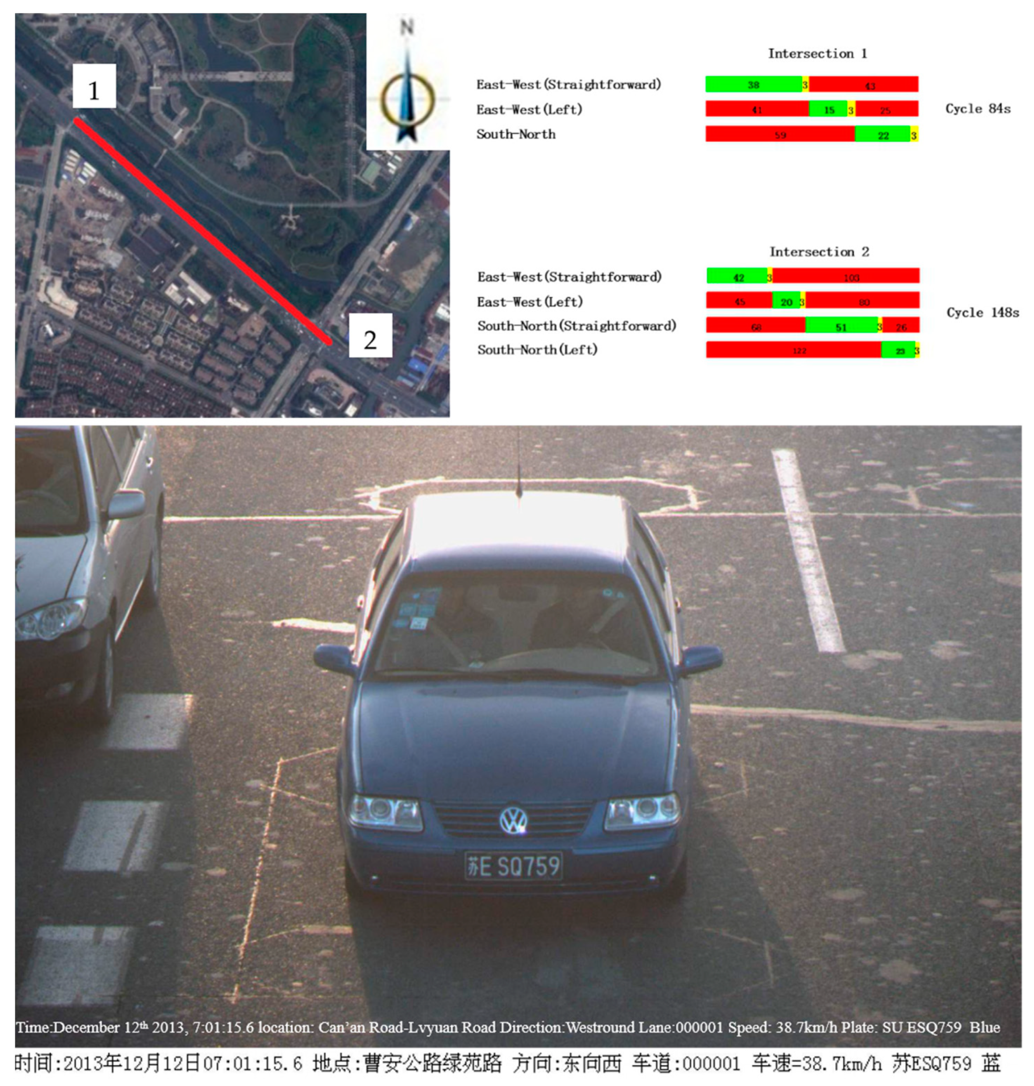
4.1. Field Data Collection

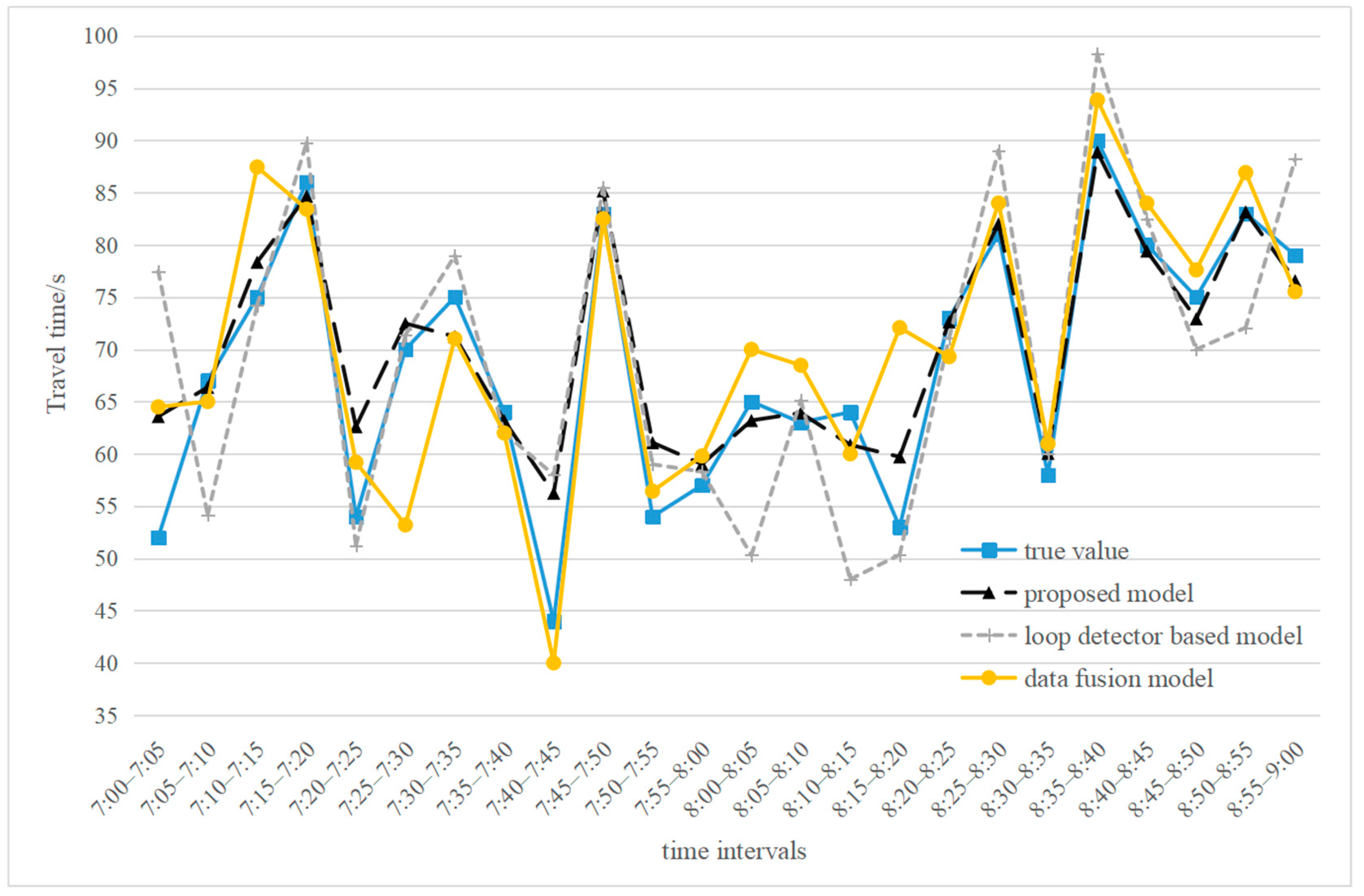
The models and algorithms presented in this paper underwent rigorous field testing. These experiments were performed on the westbound link of an approximately 767-meter section of Cao’an Road in Shanghai, China. The tests were conducted during the morning peak hour, specifically from 7:00 a.m. to 9:00 a.m. on 12 December 2013 (Thursday). To obtain accurate measurements of travel time, an automatic vehicle license plate recognition system was utilized to capture the true values (Figure 5). One floating car was used, whose license plate was shown in Figure 5. The driver was asked to follow the preceding vehicle while driving.

Utilizing the FCD, the trajectory of FCD during peak hours was calculated (Figure 6). During the 2-hour study period, 14 pieces of trajectory data were collected. One color in Figure 6 represents one trajectory. The trends observed in the FCD trajectory during peak hours align closely with the hypothesis that travel time is composed of an accelerating section, a constant-speed section, and a decelerating section (Figure 2).

In the computation of $V_{max,k}$ and $L_{1,k}$, the relative speed of FCD was employed. Relative speed refers to the ratio between the speed at the calculation location of the i-th vehicle and $V_{max}$ of the i-th vehicle throughout the link. It was determined that when 90% of the floating cars attained a relative speed of 0.9 at a specific point located at a distance h from the upstream stop line, the value of $L_{1,k}$ was deemed to be h. Additionally, the value of $V_{max,k}$ was derived by calculating the average of the maximum speeds observed in the FCD.

4.2. Data Analysis

In this paper, the following two methods were used to verify our method: a travel time estimation model with loop detector data [41], and a data fusion method [42]. Note that only 14 trajectories were captured in a 2-hour period. It indicated that the floating car was on the study link every 8 min. Thus, the low sample size can hardly support the analysis based only on the GPS data [43].

The results of the travel time estimation are presented in Figure 7, and

Table 1. Comparison between results of three models.

Study Intervals	True Value	APE%
		Proposed Model	Loop Detector Based Model	Data Fusion Model
7:00–7:05	52	22.27	49.00	24.04
7:05–7:10	67	−0.94	−19.13	−2.99
7:10–7:15	75	4.46	−1.07	16.60
7:15–7:20	86	−1.55	4.37	−3.00
7:20–7:25	54	15.94	−5.11	9.63
7:25–7:30	70	3.55	1.97	−24.00
7:30–7:35	75	−5.03	5.29	−5.31
7:35–7:40	64	−1.27	−3.11	−3.13
7:40–7:45	44	27.82	31.82	−9.09
7:45–7:50	83	2.61	3.01	−0.60
7:50–7:55	54	13.11	9.26	4.50
7:55–8:00	57	3.54	2.28	4.91
8:00–8:05	65	−2.77	−22.62	7.69
8:05–8:10	63	1.46	3.37	8.70
8:10–8:15	64	−4.90	−25.00	−6.25
8:15–8:20	53	12.67	−5.00	36.00
8:20–8:25	73	−0.50	−2.60	−5.07
8:25–8:30	81	1.25	9.93	3.70
8:30–8:35	58	3.55	3.45	5.14
8:35–8:40	90	−1.24	9.20	4.30
8:40–8:45	80	−0.73	3.13	5.00
8:45–8:50	75	−2.76	−6.67	3.47
8:50–8:55	83	0.20	−13.16	4.72
8:55–9:00	79	−3.06	11.65	−4.41
Mean Absolute Deviation		5.72	10.47	8.43

shows the absolute percentage error (APE), which is calculated by the following equation:

$$\mathrm{APE}={\displaystyle \frac{\mathrm{Estimation}-\mathrm{Observation}}{\mathrm{Observation}}}\times 100\%$$

(23)

The mean absolute error (MAE) is defined as the average absolute difference between each true value and estimated link travel time of different methods.

Blue diamonds, connected by a blue line, represent the observed average travel time for each 5-minute interval. In contrast, black triangles denote the estimated average travel time calculated by the proposed model (Figure 7). Grey crosses and orange circles represent the estimated average travel time calculated by the travel time estimation model with loop detector data and the data fusion method, respectively.

The following several key observations emerge (Figure 7 and Table 1): (1) The trend of the estimated travel time of three models aligns well with the observed data. (2) The proposed model demonstrates high accuracy in estimating average travel time, with APE values generally falling within ±5%, excluding a few outliers in gray shadow. (3) The maximal errors of the proposed model, model with loop detector data, and the data fusion method are 27.82%, 49.00%, and 36.00%. It indicates that the proposed model has better reliability than the other two models. (4) Among the three models, the proposed model had the lowest MAE, as 5.72%, followed by that of the data fusion method as 8.43%, and the model with loop detector data as 10.47%.

For the proposed model, in cases where the APE falls between 10% and 20%, the estimation values exceed the true values. Notably, these instances occur when the actual travel time is less than 55 s. This suggests that the proposed model may be less effective in handling less constrained traffic flows, which consistently exhibit shorter travel times compared to other cases.

5. Conclusions

In this study, we introduced a method for estimating real-time travel time on urban arterials fusing the data of loop detectors and probe vehicles. Considering the traffic flow characteristics, the travel time of links was divided into the following three distinct segments: accelerating, constant-speed, and decelerating phases. For the acceleration segment, travel time is determined based on vehicle speed and location functions. In the constant-speed segment, an enhanced BPR function is employed. Lastly, the deceleration segment accounts for both the time spent traversing signal control zones and approach delays. The approach delays were computed by an improved LWR shockwave theory. To validate our model, we compared the estimated travel times against field data collected via automatic license plate recognition. We also compared the proposed model with other two models, i.e., a travel time estimation model with loop detector data and a data fusion model. The results indicate a satisfactory level of accuracy, with an APE of approximately 5% for most cases. The results also show that our proposed method has better performance than the other two methods. However, our analysis suggests that the model may be less effective in less constrained traffic scenarios.

The study’s limitations are as follows:

(1)

The proposed model posits that travel time is decomposed into three distinct phases, which are typically congruent with Floating Car Data (FCD) trajectories. Nonetheless, the model acknowledges that variables such as arterial link length and prevailing traffic conditions may exert a significant influence on this segmentation.

(2)

The current model predominantly concentrates on through traffic, thereby necessitating subsequent research to elucidate the impact of turning behavior on the estimation of travel time and the precision of the model.

(3)

The model in question leverages probe data captured at one-second intervals. Although the model is capable of incorporating extended observation intervals, there exists a potential trade-off between the frequency of data collection and the fidelity of the travel time estimations.

(4)

The case study conducted indicates a positive correlation between an increased number of floating cars and enhanced estimation accuracy. However, the precise effect of the FCD sample size on this metric requires further elucidation.

(5)

The model necessitates data from both the current (k) and the subsequent (k + 1) links to facilitate precise travel time estimations. Acquiring data pertaining to the latter present certain challenges. It is imperative for future research to investigate alternative data procurement avenues or methodologies that may ameliorate this constraint.

References

1. Li, W.; Chuanjiu, W.; Xiaorong, S.; Yuezu, F. Probe vehicle sampling for real-time traffic data collection. In Proceedings of the IEEE Intelligent Transportation Systems, Vienna, Austria, 13–15 September 2005; pp. 222–224. [Google Scholar]
2. Tang, J.; Hu, J.; Hao, W.; Chen, X.; Qi, Y. Markov Chains based route travel time estimation considering link spatio-temporal correlation. Phys. A Stat. Mech. Its Appl. 2020, 545, 123759. [Google Scholar] [CrossRef]
3. Tang, J.; Yang, Y.; Qi, Y. A hybrid algorithm for urban transit schedule optimization. Phys. A Stat. Mech. Its Appl. 2018, 512, 745–755. [Google Scholar] [CrossRef]
4. Zong, F.; Tian, Y.; He, Y.; Tang, J.; Lv, J. Trip destination prediction based on multi-day GPS data. Phys. A Stat. Mech. Its Appl. 2019, 515, 258–269. [Google Scholar] [CrossRef]
5. Chen, M.; Chien, S. Dynamic freeway travel-time prediction with probe vehicle data: Link based versus path based. Transp. Res. Rec. 2001, 1768, 157–161. [Google Scholar] [CrossRef]
6. Feng, W.; Bigazzi, A.Y.; Kothuri, S.; Bertini, R.L. Freeway sensor spacing and probe vehicle penetration: Impacts on travel time prediction and estimation accuracy. Transp. Res. Rec. 2010, 2178, 67–78. [Google Scholar] [CrossRef]
7. Rahmani, M.; Jenelius, E.; Koutsopoulos, H.N. Floating car and camera data fusion for non-parametric route travel time es-timation. In Proceedings of the IEEE International Conference on Intelligent Transportation Systems, Qingdao, China, 8–11 October 2014; IEEE: Piscataway Township, NJ, USA, 2014. [Google Scholar]
8. Ma, C.; He, R.; Zhang, W. Path optimization of taxi carpooling. PLoS ONE 2018, 13, e0203221. [Google Scholar] [CrossRef] [PubMed]
9. Lu, L.; Wang, J.; He, Z.; Chan, C.-Y. Real-time estimation of freeway travel time with recurrent congestion based on sparse detector data. IET Intell. Transp. Syst. 2018, 12, 2–11. [Google Scholar] [CrossRef]
10. van Lint, J.W.C.; van der Zijpp, N.J. Improving a Travel-Time Estimation Algorithm by Using Dual Loop Detectors. Transp. Res. Rec. J. Transp. Res. Board 2003, 1855, 41–48. [Google Scholar] [CrossRef]
11. Zhang, C.; Chen, B.Y.; Lam, W.H.K.; Ho, H.W.; Shi, X.; Yang, X.; Ma, W.; Wong, S.C.; Chow, A.H.F. Vehicle Re-identification for Lane-level Travel Time Estimations on Congested Urban Road Networks Using Video Images. IEEE Trans. Intell. Transp. Syst. 2022, 23, 12877–12893. [Google Scholar] [CrossRef]
12. Xia, D.; Zheng, L.; Tang, Y.; Cai, X.; Chen, L.; Liu, W.; Sun, D. Link-Based Traffic Estimation and Simulation for Road Networks Using Electronic Registration Identification Data. IEEE Trans. Veh. Technol. 2022, 71, 8075–8088. [Google Scholar] [CrossRef]
13. Zhu, Y.; He, Z.; Zhang, X. Optimal number and locations of automatic vehicle identification sensors considering link travel time estimation. IET Intell. Transp. Syst. 2023, 17, 1846–1859. [Google Scholar] [CrossRef]
14. Osei, K.K.; Adams, C.A.; Sivanandan, R.; Ackaah, W. Modelling of segment level travel time on urban roadway arterials using floating vehicle and GPS probe data. Sci. Afr. 2022, 15, e01105. [Google Scholar] [CrossRef]
15. Gündüz, G.; Acarman, T. Vehicle Travel Time Estimation Using Sequence Prediction. Promet-Traffic Transp. 2020, 32, 1–12. [Google Scholar] [CrossRef]
16. Jedwanna, K.; Boonsiripant, S. Evaluation of Bluetooth Detectors in Travel Time Estimation. Sustainability 2022, 14, 4591. [Google Scholar] [CrossRef]
17. Lee, K.; Prokhorchuk, A.; Dauwels, J.; Jaillet, P. Estimation of travel time from taxi GPS data. In Proceedings of the 2017 IEEE Symposium Series on Computational Intelligence (SSCI), Honolulu, HI, USA, 27 November–1 December 2017; pp. 1–6. [Google Scholar] [CrossRef]
18. Sun, T.; Zhao, K.; Zhang, C.; Chen, M.; Yu, X. PR-LTTE: Link travel time estimation based on path recovery from large-scale incomplete trip data. Inf. Sci. 2020, 589, 34–45. [Google Scholar] [CrossRef]
19. Cao, J.; Du, Y.; Mao, L.; Ji, Y.; Ma, F.; Wang, X. Improved DTTE Method for Route-Level Travel Time Estimation on Freeways. J. Transp. Eng. Part A Syst. 2021, 148, 04021113. [Google Scholar] [CrossRef]
20. Li, A.; Lam, W.H.; Ma, W.; Wong, S.; Chow, A.H.; Tam, M.L. Real-time estimation of multi-class path travel times using multi-source traffic data. Expert Syst. Appl. 2024, 237, 121613. [Google Scholar] [CrossRef]
21. Jin, G.; Wang, M.; Zhang, J.; Sha, H.; Huang, J. STGNN-TTE: Travel time estimation via spatial–temporal graph neural network. Future Gener. Comput. Syst. 2022, 126, 70–81. [Google Scholar] [CrossRef]
22. Kim, H.; Ye, L. Bayesian Mixture Model to Estimate Freeway Travel Time under Low-Frequency Probe Data. Appl. Sci. 2022, 12, 6483. [Google Scholar] [CrossRef]
23. Choi, K.; Chung, Y. A Data Fusion Algorithm for Estimating Link Travel Time. J. Intell. Transp. Syst. 2002, 7, 235–260. [Google Scholar] [CrossRef]
24. Li, H.; Yang, X. Data fusion method on modifying sampling bias of floating cars. J. Tongji Univ. (Nat. Sci.) 2012, 40, 1498–1503. [Google Scholar] [CrossRef]
25. Liang, Z.; Ling-Xiang, Z. Link Travel Time Estimation Model Fusing Data from Mobile and Stationary Detector Based on BP Neural Network. In Proceedings of the 2006 International Conference on Communications, Circuits and Systems, Guilin, China, 25–28 June 2006; pp. 2146–2149. [Google Scholar]
26. Bhaskar, A.; Chung, E.; Dumont, A.-G. Average Travel Time Estimations for Urban Routes that Consider Exit Turning Movements. Transp. Res. Rec. 2012, 2308, 47–60. [Google Scholar] [CrossRef]
27. Celikoglu, H.B. Flow-Based Freeway Travel-Time Estimation: A Comparative Evaluation within Dynamic Path Loading. IEEE Trans. Intell. Transp. Syst. 2013, 14, 772–781. [Google Scholar] [CrossRef]
28. Wang, S.; Patwary, A.; Huang, W.; Lo, H.K. A general framework for combining traffic flow models and Bayesian network for traffic parameters estimation. Transp. Res. Part C Emerg. Technol. 2022, 139, 103664. [Google Scholar] [CrossRef]
29. Wang, S.; Huang, W.; Lo, H.K. Combining shockwave analysis and Bayesian Network for traffic parameter estimation at signalized intersections considering queue spillback. Transp. Res. Part C Emerg. Technol. 2020, 120, 102807. [Google Scholar] [CrossRef]
30. Claudel, C.; Hofleitner, A.; Mignerey, N.; Bayen, A. Guaranteed bounds on highway travel times using probe and fixed data. In Proceedings of the 88th TRB Annual Meeting Compendium of Papers, Washington, DC, USA, 11–15 January 2009. [Google Scholar]
31. Berkow, M.; Monsere, C.M.; Koonce, P.; Bertini, R.L.; Wolfe, M. Prototype for Data Fusion Using Stationary and Mobile Data. Transp. Res. Rec. 2009, 2099, 102–112. [Google Scholar] [CrossRef]
32. Zheng, L.; Ma, H.; Wu, B.; Wang, Z.; Cai, Q. Estimation of Travel Time of Different Vehicle Types at Urban Streets Based on Data Fusion of Multisource Data. In Proceedings of the 14th COTA International Conference of Transportation Professionals, Changsha, China, 4–7 July 2014. [Google Scholar]
33. He, N.; Zhao, S. Discussion on Influencing Factors of Free-flow Travel Time in Road Traffic Impedance Function. Procedia-Soc. Behav. Sci. 2013, 96, 90–97. [Google Scholar] [CrossRef]
34. Pan, Y.; Zheng, H.; Guo, J.; Chen, Y. Modified Volume-Delay Function Based on Traffic Fundamental Diagram: A Practical Calibration Framework for Estimating Congested and Uncongested Conditions. J. Transp. Eng. Part A Syst. 2023, 149, 4023112.1–4023112.14. [Google Scholar] [CrossRef]
35. Branston, D. Link capacity functions: A review. Transp. Res. 1976, 10, 223–236. [Google Scholar] [CrossRef]
36. Lighthill, M.J.; Whitham, G.B. On kinematic waves. ii. A theory of traffic flow on long crowded roads. Proc. R. Soc. A Math. Phys. Eng. Sci. 1985, 229, 317–345. [Google Scholar]
37. Sakhare, R.S.; Li, H.; Bullock, D.M. Methodology for the Identification of Shock Wave Type and Speed in a Traffic Stream Using Connected Vehicle Data. Futur. Transp. 2023, 3, 1147–1174. [Google Scholar] [CrossRef]
38. Zhang, Y.; Kouvelas, A.; Makridis, M.A. A time-varying shockwave speed model for reconstructing trajectories on freeways using Lagrangian and Eulerian observations. Expert Syst. Appl. 2024, 253, 124298. [Google Scholar] [CrossRef]
39. Wang, W. Practical speed-flow relationship model of highway traffic-flow. Dongnan Daxue Xuebao/J. Southeast Univ. (Nat. Sci. Ed.) 2003, 33, 487–491. [Google Scholar]
40. Mousa, R.M. Analysis and Modeling of Measured Delays at Isolated Signalized Intersections. J. Transp. Eng. 2002, 128, 347–354. [Google Scholar] [CrossRef]
41. Bing, Q.; Qu, D.; Chen, X.; Pan, F.; Wei, J. Arterial travel time estimation method using SCATS traffic data based on KNN-LSSVR model. Adv. Mech. Eng. 2019, 11, 1687814019841926. [Google Scholar] [CrossRef]
42. Hu, X.; Yang, D. Link travel time estimation based on data fusion. J. Transp. Inf. Saf. 2011, 29, 92–98. [Google Scholar] [CrossRef]
43. Loe, L.E.; Bonenfant, C.; Meisingset, E.L.; Mysterud, A. Effects of spatial scale and sample size in GPS-based species distribution models: Are the best models trivial for red deer management? Eur. J. Wildl. Res. 2012, 58, 195–203. [Google Scholar] [CrossRef]
Figure 1. The definition of the link applied to estimating link travel time.
Sustainability 16 07845 g001
Figure 2. Driving behavior along an arterial link.
Sustainability 16 07845 g002
Figure 3. Calculation of approach delay using shockwave theory.
Sustainability 16 07845 g003
Figure 4. Calculation of approach delay using improved shockwave theory.
Sustainability 16 07845 g004
Figure 5. Information of the test site and picture from the automatic vehicle license plate recognition system.
Sustainability 16 07845 g005
Figure 6. Trajectory of FCD at peak hour.
Sustainability 16 07845 g006
Figure 7. Testing results.
Sustainability 16 07845 g007