Analysis of PM₁₀ Substances via Intuitionistic Fuzzy Decision-Making and Statistical Evaluation

Abstract

Air pollution is a situation that negatively affects the health of humans and all living things in nature and causes damage to the environment. The most important cause of air pollution is the amount and density of substances called “particulate matter” above guidelines. Particulate matter (PM) are mixed liquid droplets and solid particles with advective diameters less than 2.5 μm (PM_2.5—fine particles) and between 2.5 and 10 μm (PM_2.5–10—coarse particles). PM₁₀ is defined as one that can remain in the air for a long time and settle in the respiratory tract, damaging the lungs. It is important to identify the underlying causes of air pollution caused by PM₁₀. In this context, these criteria need to be evaluated to minimize the negative effects of PM₁₀. In the study, monthly average PM₁₀ data obtained from the Air Quality Monitoring Station in Kocaeli, Türkiye, between 2017 and 2023 are used. After determining the criteria for PM₁₀, the criteria are prioritized with the Intuitionistic Fuzzy AHP (IF-AHP) method by taking decision-maker opinions. The proposed decision-making model aims to guide obtaining and focusing on the important causes of out-of-limit and dangerous PM₁₀ concentrations in the air. Additionally, PM₁₀ data is analyzed in the context of COVID-19 and a statistical analysis is conducted. One-way Analysis of Variance (ANOVA) is used to evaluate whether there is a significant difference in average monthly data over the years. The Games–Howell test, one of the post-hoc tests, is used for determining differences between groups (years). In addition, monthly PM₁₀ values for the future are estimated using the Expert Modeler tool in the software IBM^® SPSS^® Statistics 22. The study is important in that it provides a focus on the criteria affecting PM₁₀ with an intuitionistic fuzzy perspective, along with statistical analysis.

1. Introduction

Since air is one of the most basic elements required for the vital functioning of humans and many living things, “air pollution” is an issue that concerns all people. Increases in the concentrations of pollutants that cause air pollution also greatly affect humans, living things, and environmental health. According to the World Health Organization (WHO), approximately seven million people in the world die every year due to air pollution-related causes such as lung cancer, heart disease, and acute respiratory diseases [1]. It is reported that air pollution is the cause of approximately 45 thousand preventable premature deaths every year in Türkiye [2]. It is possible to group air pollutants into gases and aerosol pollutants. Particulate matter (PM₁₀ and PM_2.5) is the most dangerous fraction of aerosol pollutants due to inhalation risks. Airborne PM is not a single pollutant but rather is a mixture of many chemical species. It is a complex mixture of solids and aerosols composed of small droplets of liquid, dry solid fragments, and solid cores with liquid coatings [3]. Particulate matter can occur naturally, such as in volcanic eruptions, dust storms, forest fires, vegetation, and sea sprays (the mixing of aerosol particles into the air by the explosion of bubbles). It can also be caused by human-made fixed and mobile structures such as vehicle exhausts, construction and demolition operations, residential fires, construction sites, and industrial sites. Particles can form in the atmosphere not only naturally or as a result of human activities, but also through the transformation of gas emissions such as sulfur oxide and nitrogen [4].

Türkiye, which is in the process of obtaining European Union (EU) membership, has harmonized its legislation with the EU and reduced the guidelines for air pollutants, bringing them to the level of the values applied in European countries. As of the beginning of 2019, the guidelines for PM₁₀ and SO₂ applied in EU countries have also come into force in Türkiye. Air quality in our cities is constantly monitored thanks to the National Air Quality Monitoring Network operated by the Türkiye Ministry of Environment and Urbanization, and the results are announced via its website and mobile application. The Ministry of Environment, Urbanization, and Climate Change has published the Türkiye Environmental Problems and Priorities Assessment Report. According to the report prepared using 2022 data; air pollution ranked first in 22 provinces of Türkiye and among the top three environmental problems in 66 provinces. It was stated that air pollution continues to increase in Türkiye [5]. Since changes in air quality need to be constantly monitored and evaluated, it is often possible to come across studies on this subject. However, when the time aspect of the work comes into play, or in other words when time passes and the work loses its currentness, the work must be repeated. The guidelines set by the WHO for the PM₁₀ pollutant is on average 15 μg/m³ (daily) and 5 μg/m³ (annually). The guidelines for PM₁₀ pollutants have been determined for Türkiye at the national level. The guidelines determined for PM₁₀ pollutants in Türkiye were the same in 2021, 2022, and 2023. These values are on average 50 μg/m³ (daily), 40 μg/m³ (winter period), and 40 μg/m³ (annually). All guidelines are given in

Table 1. PM₁₀ guidelines for WHO and Türkiye national values based on period.

Pollutant	Period	WHO	Türkiye National Values
PM10	Daily	15 μg/m3	50 μg/m3
	Annually	5 μg/m3	40 μg/m3
	Winter Period	-	40 μg/m3

[6,7,8].

According to Table 1, the difference between WHO and Türkiye national guidelines is remarkable and is worth examining and taking precautions. It is important to scientifically examine the parameters affecting air pollution to monitor air pollution and minimize the effects of pollutants such as PM₁₀. Air pollution, defined as the presence of pollutants in the atmosphere at levels and durations that may harm human health, animals, plants, natural environments, and commercial and private properties, needs to be monitored and evaluated, and its distribution and change analyzed [9,10]. There are many studies in the literature examining the parameters affecting PM₁₀ concentrations and pollution relationships.

Eroğlu [11] aimed to determine the extent of air pollution in the Çerkezköy and Kapaklı districts of Türkiye and the natural and human factors that cause air pollution. For this purpose, measurement values from Çerkezköy Air Quality Monitoring Station between 2013 and 2023 were used. Annual average PM₁₀, PM_2.5, SO₂, NO₂, NO_x, and NO values were measured in Çerkezköy and Kapaklı. It has been determined that the annual averages of PM₁₀ and NO_x among these pollutants are higher than the guidelines for Türkiye, the EU, and the WHO. In terms of the sustainability of the human–space relationship in Çerkezköy and Kapaklı districts, taking into account the factors that cause air pollution, practices have been suggested to solve the problems. Birim et al. [12] examined correlations between PM₁₀ pollutant data and meteorological parameters such as temperature, relative humidity, and wind speed and direction. Two different regions of Izmir province in Turkey were used as case studies and PM₁₀ data were evaluated between 1 January 2017 and 31 December 2021. The t-test was used to statistically determine the relationship between PM₁₀ pollutant data and meteorological parameters. As a further study, to assess the practical significance of parameters, the effect size method was employed. Relative humidity emerged as the most effective parameter based on correlation coefficient calculations. Zajusz-Zubek et al. [13] used dendrogram (DE), heat map (HM), and principal component analysis (PCA) methods to determine possible emission factors from PM₁₀. In their study, PCA was shown to be the most useful statistical tool for PM₁₀ factors. The main sources identified by the PCA are coal combustion, resuspension of soil and road dust, pesticide use, and waste incineration. Ul-Saufie et al. [14] used machine learning approaches in their study, apart from statistical method feature selection, to predict PM₁₀ concentrations in Malaysia. The impact variables of the prediction model were investigated to compare the prediction model performance and predict the daily PM₁₀ concentrations. In the study, weight-guided and genetic algorithm evolution, predictive analytical multiple linear regression (MLR), and artificial neural network (ANN)) were applied. The methods were compared based on The Root Mean Square Error (RMSE) and Absolute Error (AE) metrics. Erener et al. [15] examined the relationship between air pollution and seasonal meteorological data in Kocaeli, Türkiye. They made evaluations by regression analysis with daily SO₂ and PM₁₀ parameters and meteorological data such as temperature, wind direction, wind speed, relative humidity, and air pressure for 2015. Bai et al. [16] conducted a study on natural and socioeconomic factors affecting air pollution along with urban air quality monitoring data from 2015 in the Yangtze River Economic Zone. As a result of the study, they concluded that topographic, meteorological, economic development and urbanization factors are related to air pollution. Some scientists have shown in their research that meteorological factors (temperature, precipitation, humidity, atmospheric pressure, wind speed, etc.) have a significant impact on air pollution [17,18]. Jiang et al. [19] concluded in their study that the topographic structure prevents the clustering and dispersion of pollutants, and it was also revealed that as population and income levels increase, factors such as fossil fuel use, the number of vehicles, urbanization, and industrialization increase, causing pollutant emissions to increase, and therefore these factors affect air pollution. Lin and Wang [20] stated that air pollution is significantly dependent on energy consumption, industrialization, and technological developments in China.

In these studies on PM₁₀ concentration values, the relationships between pollutants and pollutant factors are examined [11,12,15,16,17,18,19,20], while in some studies, the success of the methods used in the estimation of pollutants is examined [13,14].

Two different methods are used to evaluate air pollution: deterministic methods and statistical methods. Although deterministic methods are methods that model physical and chemical processes such as discharge, accumulation, or transfer processes of pollutants using meteorological, emission, and chemistry models, the accuracy of these methods varies depending on the quality and scale of the data used and it takes a long time to apply these methods to big data. The importance of statistical methods, which compensate for the shortcomings and weaknesses of deterministic methods, is increasing in studies [21]. Statistical methods have also been used in the literature, especially in studies involving the PM₁₀ pollutant. Some of these methods include estimation and examination of the relationship between variables, and some include statistical analysis according to significance levels [22,23,24,25]. There are many decision-making problems in daily life. Multi-criteria decision-making (MCDM) methods, considered among deterministic methods, allow decision-makers to choose among a separate set of decisions or criteria or to prioritize these criteria or decisions. An exemplary study [26] on PM pollutants is on the material selection and evaluation of PM sensors. They proposed an analytical framework based on multi-criteria decision-making to evaluate and select the most suitable materials for the fabrication of PM sensors. In order to demonstrate the suitability of the analytical framework in the study, an empirical study was conducted based on recent research and received the opinions of 13 different decision-makers. A hybrid model has been developed using frequently used MCDM techniques such as DEMATEL, Analytic Network Process (ANP), and VIKOR. In many studies involving deterministic MCDM methods, there is actually a process of digitizing specific judgments, which essentially enables difficult decision processes to be concretized. In other studies, MCDM methods and even fuzzy logic have been included among the deterministic methods [27,28,29].

The COVID-19 pandemic has had serious negative effects on human health and the world economy; however, limiting social and economic activities also mediated the reduction in air pollution [30] because the main source of air pollution is anthropogenic activities [31]. It appears that the measures taken reduced the volume of these activities to a large extent. For example, during quarantine, mobility decreased by approximately 50% in Italy and 79% in France [32,33]. Particularly with travel restrictions and flexible working opportunities, the density in the transportation sector, which constitutes approximately one-quarter of total greenhouse gas emissions and is considered the main cause of air pollution in cities, was greatly reduced [34]. The decrease in emission sources of air pollutants has played an encouraging role in research conducted to determine changes in air quality.

In this study, the criteria affecting PM₁₀ values are examined in detail; the criteria weights are obtained from the IF-AHP perspective, and the criteria importance ranking is determined. In this context, the criterion or criteria affecting PM₁₀ that will be focused on and evaluated are discussed from an intuitionistic fuzzy decision-making perspective. This point is the motivation for the study as it fills the gap in the literature. In addition to this decision analysis, a statistical evaluation was also presented using 7-year PM₁₀ values covering the COVID-19 period in Kocaeli, Türkiye. Determination of whether there was a significant difference between the average data is evaluated using one-way ANOVA. PM₁₀ concentration values were estimated monthly based on statistical data analysis using Expert Modeler in the IBM^® SPSS^® Statistics 22 software. In the Section 2 of the study, the materials and methods are presented. The Section 3 covers the results. The Section 4 contains a discussion. Conclusions are given in the Section 5.

2. Materials and Methods

A flow diagram of this study’s process is presented in Figure 1.

The main source of innovation in this study is to provide decision-makers with a roadmap on PM₁₀ by using deterministic and statistical methods together and to fill the literature gap in this field. The absolute data obtained will be analyzed statistically and a decision model that includes criterion prioritization will be presented to decision-makers in line with the subjective criteria in the decision process.

2.1. Study Area and Data

Kocaeli province is located in the Marmara Region of Türkiye. Figure 2 shows the location of Kocaeli. Kocaeli is the 10th most populous city in Türkiye and according to 2023 TURKSTAT data, its population is 2,102,907 people and its area is 3626 km² [35].

Since the negative effects of air pollution on human health are known, air quality sampling data should be collected at a certain frequency to determine the level of emissions. For this purpose, 125 air pollution surveys were conducted in 81 provinces between 2005 and 2007 by the Türkiye Ministry of Environment, Urbanization, and Climate Change to measure air pollution accurately, establish air pollution policies in all provinces, and improve air quality in the provinces within the framework of these policies compared to the values of the previous year. A quality measurement station was established and a National Air Quality Monitoring Network was established throughout Türkiye. Particulate matter (PM₁₀) parameters can be measured fully automatically in all established air pollution measurement stations. Measurement data collected at measurement stations are monitored and transferred to the Ministry’s Environmental Reference Laboratory Data Processing Center via GSM Modems over a special network (VPN) belonging to the Türkiye Ministry of Environment, Urbanization, and Climate Change and published simultaneously [37]. Verification studies are carried out by examining the data received from the stations in the form of hourly averages, and monthly and annual reports are prepared and published with the data in question. These measurements have been made continuously at stations in Kocaeli province since 1987. Air pollution parameters are measured hourly at air quality monitoring stations. There are a total of 12 measurement stations in Kocaeli province under the control of the Türkiye Ministry of Environment, Urbanization, and Climate Change [36]. Air quality monitoring stations are established in four different categories: urban, traffic, industrial, and rural. At the air quality measurement station, PM₁₀ concentration values are measured with automatic devices in accordance with international standards. The Kocaeli air quality monitoring station is shown in Figure 3. The station in Figure 3 is an urban-type station.

Monthly average PM₁₀ concentration values for the years 2017–2023 obtained from the Kocaeli air quality monitoring station (central) are given in

Table 2. Monthly average PM₁₀ concentration values for the years 2017–2023 obtained from the Kocaeli air quality monitoring station (central) (μg/m³).

	Years	2017	2018	2019	2020	2021	2022	2023
Months
January		37.89	69.94	59.45	43.18	44.67	39.85	49.55
February		74.28	59.72	58.4	44.53	47.74	52.45	46.42
March		69.05	77.92	51.69	45.11	38.3	51.08	34.51
April		47.29	71.63	45.47	39.39	42.58	55.93	34.2
May		39.08	49.6	58.05	39.24	37.77	40.1	30.41
June		47.22	55.1	51.42	39.51	37.68	34.81	23.16
July		42.61	58.52	40.78	31.59	40.25	29.9	33.52
August		42.53	54.11	41.98	30.73	38.91	39.89	39.31
September		53.8	54.39	45.53	38.4	37.24	39.69	29.84
October		76.98	67.92	55.55	45.54	39.74	39.22	53.85
November		86.18	57.28	78.06	39.5	63.62	55.72	42.35
December		85.29	67.32	70.07	44.72	41.82	64.02	61.02

.

Monthly average values are calculated based on the measured “daily” PM₁₀ concentration values in Table 2. The numbers of days exceeding Türkiye’s guideline of 50 μg/m³ for each year are as follows: “2017: 164 days”; “2018: 225 days”; “2019: 164 days”; “2020: 75 days”; “2021: 90 days”; “2022: 119 days”; “2023: 84 days”. While the maximum number of limit-day exceedances was in 2018, the minimum number of limit-day exceedances was in 2020.

Statistical descriptives for Kocaeli’s monthly average PM₁₀ concentration values in Table 2 are calculated using the IBM^® SPSS^® Statistics 22 software. The findings obtained are given in

Table 3. Statistical descriptives for Kocaeli’s average PM₁₀ concentration values by years.

Year		Mean	Std. Deviation (Standard Deviation)	Std. Error (Standard Error)	Max	Min
2017	12	58.52	18.51	5.34	86.18	37.89
2018	12	61.95	8.70	2.51	77.92	49.60
2019	12	54.70	11.18	3.23	78.06	40.78
2020	12	40.12	4.96	1.43	45.54	30.73
2021	12	42.53	7.36	2.12	63.62	37.24
2022	12	45.22	10.26	2.96	64.02	29.90
2023	12	39.84	11.10	3.20	61.02	23.16
Total	84	48.98	13.65	1.49	86.18	23.16

.

According to Table 2 and Table 3, the highest monthly average PM₁₀ concentration value was recorded in “November 2017”, at “86.18 μg/m³”, while the lowest monthly average PM₁₀ concentration value was recorded in “June 2023”, at “23.16 μg/m³”. According to Table 3, the highest standard deviation of PM₁₀ concentration values was calculated for 2017, with a value of 18.51, while the lowest standard deviation was calculated for 2020, with a value of 4.96. The highest annual average value, 61.95, was achieved in 2018 when the COVID-19 pandemic had not yet started. Due to restrictions around the world, the annual average PM₁₀ concentration value decreased significantly in 2020. The annual average PM₁₀ concentration value started to increase again in 2021 and 2022. In 2023, it showed a serious decrease again. It can be assumed that this decrease is related to the introduction of various measures against air pollution and the adoption of remote working principles by most businesses due to the COVID-19 pandemic. In this context, it is important that the criteria affecting PM₁₀ concentration be considered in a region-specific manner and be examined in detail by decision-makers. In this study, the selection of some criteria affecting PM₁₀ concentration values is made using the “brainstorming” method by decision-makers who evaluated the literature. For this purpose, the scale that will be detailed in the next section is used. Decision-makers are asked to compare the evaluation criteria pairwise and the IF-AHP algorithm is included in the process. It is aimed at obtaining criterion weights for each criterion at the end of the IF-AHP process steps. Thus, the order of importance of the criteria from the decision-making perspective can be obtained. In addition, statistical analysis is performed on actual PM₁₀ concentration values, and one-way ANOVA is used to evaluate whether there is a significant difference between average PM₁₀ concentration values in the context of COVID-19. The results obtained using one-way ANOVA are evaluated and prospective monthly PM₁₀ concentration “prediction” values are handled using Expert Modeler.

In the following sections, IF-AHP, one-way ANOVA, and Expert Modeler methodologies are presented.

2.2. Intuitionistic Fuzzy AHP (IF-AHP)

The AHP method was developed by Professor Thomas L. Saaty and is used for decision-making problems. AHP is a methodology based on one-to-one comparisons of the criteria and sub-criteria affecting the decision according to their degree of importance, using a binary comparison scale in any decision problem. The AHP method also aims to prioritize by distinguishing between alternative options to meet interconnected goals [38]. However, AHP cannot fully reflect the functioning of the complex human thought system. For this reason, the method has been used by many researchers in problem-solving by combining it with the fuzzy logic approach [39,40,41]. In the following periods, the uncertain and hesitant situations of decision-makers and the decision environment brought about the search for heuristics in the fuzzy AHP method. By developing intuitionistic fuzzy set theory, this approach has been integrated with the AHP method and investigated by several researchers [42]. Abdullah and Najib [42] proposed a new heuristic fuzzy AHP with a new pairwise matching comparison matrix evaluation preference scale. This new preference scale led to the proposal of a new consistency test for matrix evaluation using the values of the degree of hesitation. The steps of the IF-AHP method presented by Abdullah and Najib are as follows:

Step 1: A hierarchical structure is created for the decision problem.

Step 2: Pairwise comparison matrices are created with the triangular intuitive fuzzy numbers preference scale in

Table 4. Triangular intuitive fuzzy numbers comparison preference scale.

Comparison Preference	AHP Preference Correspondence	Triangular Intuitive Fuzzy Numbers	Opposite Triangular Intuitive Fuzzy Numbers
Equal Important	1	(0.02  0.18  0.80)	(0.02  0.18  0.80)
Middle	2	(0.06  0.23  0.70)	(0.23  0.06  0.70)
Somewhat Important	3	(0.13  0.27  0.60)	(0.27  0.13  0.60)
Middle	4	(0.22  0.28  0.50)	(0.28  0.22  0.50)
Strongly Important	5	(0.33  0.27  0.40)	(0.27  0.33  0.40)
Middle	6	(0.47  0.23  0.30)	(0.23  0.47  0.30)
Very Strongly Important	7	(0.62  0.18  0.20)	(0.18  0.62  0.20)
Middle	8	(0.80  0.10  0.10)	(0.10  0.80  0.10)
Absolutely Important	9	(1     0     0)	(0     1     0)

. In the decision-making process, evaluation criteria are analyzed by decision-makers using pairwise comparison. For this purpose, in the normal AHP method, the criteria are compared with each other in pairs based on the “Comparison Preference” and “AHP Preference Correspondence” columns in Table 4. Inverse reciprocals are expressed as fractions. In the IF-AHP method, a pairwise comparison of evaluation criteria is made with triangular and opposite triangular intuitive fuzzy number logic. The equivalents of the AHP comparison scale in IF-AHP are also included in Table 4. As stated in Section 2.1, each decision-maker subjects each evaluation criterion to a pairwise comparison.

Step 3: The weights of decision-makers are determined. The degree of importance of the decision-makers to the decision problem is also expressed by linguistic variables. Triangular intuitive fuzzy numbers defined for linguistic variables are given in

Table 5. Linguistic variables and triangular intuitive fuzzy number correspondence for the importance levels of decision-makers.

Linguistic Variables	Triangular Intuitive Fuzzy Number Correspondence
Very important	(0.90  0.05  0.05)
Important	(0.75  0.20  0.05)
Somewhat Important	(0.50  0.40  0.10)
Insignificant	(0.25  0.60  0.15)
Very unimportant	(0.10  0.80  0.10)

. $D_k({\mu }_k,v_k, {\tau }_k)$ is the expression of the degree of importance of expertise of the decision maker “k” for the decision in terms of an intuitive fuzzy number. The aim is to include different levels of expertise in the decision-making process. The importance levels of the decision-makers in the decision-making group in the process are determined according to the linguistic variables and their equivalents in Table 5.

The weight of the k decision-maker is calculated using Equation (1) [43].

$${\lambda }_k={\displaystyle \frac{{\mu }_k+{\tau }_k\left(\frac{{\mu }_k}{{\mu }_k+v_k}\right)}{{\sum }_{k=1}^l({\mu }_k+{\tau }_k\left(\frac{{\mu }_k}{{\mu }_k+v_k}\right))}}$$

(1)

where

${\sum }_{k=1}^l{\lambda }_k=1,k=(\mathrm{1,2},\dots l)$.

Step 4: The aggregated intuitive fuzzy decision matrix based on the decision-maker’s opinion is created using the intuitive fuzzy weighted average (IFWA) operator developed by Xu [44].

The combination form of the IFWA operator is given in Equation (2), where $R^{\left(k\right)}={{(r}_{ij}^k)}_{mxn}$ is the intuitive fuzzy decision matrix of the $k$ decision-maker and $\lambda ={(\lambda }_1,{\lambda }_2,{\dots \lambda }_n)$ is the weight of all decision-makers.

$$r_{ij}={IFWA}_{\lambda }(r_{ij}^{\left(1\right)},r_{ij}^{\left(2\right)},\dots ,r_{ij}^{\left(l\right)})={(\lambda }_1{r}_{ij}^{\left(1\right)}\left(+\right){ \lambda }_2{r}_{ij}^{\left(2\right)}\left(+\right)\dots { \left(+\right) \lambda }_l{r}_{ij}^{\left(l\right)})$$

(2)

$r_{ij}=(1-{\prod }_{k=1}^l{(1-{\mu }_{ij}^{\left(k\right)})}^{{\lambda }_k}$, ${\prod }_{k=1}^l{(v_{ij}^{\left(k\right)})}^{{\lambda }_k}$, ${\prod }_{k=1}^l{(1-{\mu }_{ij}^{\left(k\right)})}^{{\lambda }_k}-{\prod }_{k=1}^l{(v_{ij}^{\left(k\right)})}^{{\lambda }_k})$.

From here to $r_{ij}={(\mu }_{ij},v_{ij},{\tau }_{ij}$);

It is expressed as;

$${\mu }_{ij}=1-{\prod }_{k=1}^l{(1-{\mu }_{ij}^{\left(k\right)})}^{{\lambda }_k}$$

$$v_{ij}={\prod }_{k=1}^l{(v_{ij}^{\left(k\right)})}^{{\lambda }_k}$$

$${\tau }_{ij}={\prod }_{k=1}^l{(1-{\mu }_{ij}^{\left(k\right)})}^{{\lambda }_k}-{\prod }_{k=1}^l{(v_{ij}^{\left(k\right)})}^{{\lambda }_k}$$

Step 5: The consistency ratio (CR) is calculated for the collective heuristic fuzzy decision matrix. Since the bulk intuitionistic fuzzy matrix contains the τ (x) value, which is the hesitation value of triangular intuitionistic fuzzy numbers, a new method is presented for calculating the consistency ratio [42]. Random index (RI) values were taken from

Table 6. RI values for the standard AHP and IF-AHP methods.

$\mathit{n}$	1–2	3	4	5	6	7	8	9
RI	0.0	0.58	0.90	1.12	1.24	1.32	1.41	1.45

presented by Saaty in the standard AHP method [45]. These RI values are also used in the IF-AHP method. According to the new method presented, CR is calculated using the equation in Equation (3). (λmax − n) in Equation (3) is the average of the τ(x) values in the aggregated intuitive fuzzy matrix of each criterion. The value of $n$ is the size of the matrix.

$$CR={\displaystyle \frac{({\lambda }_{max}-n)/n-1}{RI}}$$

(3)

The matrix is confirmed to be consistent if the CR value does not exceed 0.10. If this value is greater than 0.10, there is an inconsistent decision matrix and, in this case, it is necessary to reconstruct the comparison matrices.

Step 6: The intuitive fuzzy entropy weights of the weighted aggregated intuitive fuzzy decision matrix are calculated using the equation given in Equation (4) and the final weights are calculated with the equation in Equation (5). Afterward, final criterion weights can be obtained by taking arithmetic averages.

$$\stackrel{̿}{\mathrm{w}}\mathrm{i}=-{\displaystyle \frac{1}{nln2}}[{\mu }_{i}ln{\mu }_i+v_{i}ln{v}_i-\left(1-{\tau }_i\right)\ln \left(1-{\tau }_i\right)-{\tau }_{i}ln2]$$

(4)

$$w_i={\displaystyle \frac{1-\stackrel{̿}{\mathrm{w}}\mathrm{i}}{n-{\sum }_{j=1}^n\stackrel{̿}{\mathrm{w}}\mathrm{i}}}, {\sum }_{j=1}^n{w}_i=1$$

(5)

2.3. One-Way ANOVA

The concept of analysis of variance used in statistics is the general name of a group method that includes many statistical methods. The simplest form of variance analysis is a one-way analysis of variance (one-way ANOVA). As with other tests, some prerequisites must be met in the application of this test. These conditions are the homogeneity of group variances and that the dependent variable consists of quantitative data. One-way ANOVA is used to analyze how independent variables interact with each other and the effect of this interaction on the dependent variable [46]. Multiple comparison post-hoc tests are divided into two groups as shown in

Table 7. Post-hoc tests used based on variance homogeneity.

Tests Using the Equal Variance Theory	Tests Using Different Variance Theory
LSD (Fisher’s significant difference test)	Tamhane Test
Bonferroni Test	Dunnet T3 Test
Tukey HSD Test	Games–Howell Test
Scheffe Test	Dunnet–C Test
Duncan Test
Dunnet Test
Waller–Duncan Test

, according to equal or different variance approaches.

In the variance homogeneity analysis results, it is said that there is a significant difference between the groups when the significance level (Sig.) value is less than 0.05. If the Sig. value is less than 0.05, it is necessary to find out which groups this difference is between using the tests in Table 7.

2.4. Expert Modeler

Expert modeler is a tool used in the IBM^® SPSS^® Statistics 22 software to choose the ideal model among exponential smoothing or ARIMA models in time series that can be used for forecasting. Often known as a skilled data analyst, an expert modeler can create complex models to analyze data and make predictions. Expert modeler allows not only the theoretical foundations of various modeling techniques but also the process of applying the selected model based on the characteristics of the data and the goals of the analysis [47]. IBM notes: “Expert Modeler provides options you can use, including restricting the set of candidate models, handling outliers, and event variables” [48]. In many studies in the literature, statistical analysis and predictions are made using Expert Modeler [47,49,50,51]. The Expert Modeler’s feature automatically determines the best Autoregressive Integrated Moving Average (ARIMA) or exponential smoothing model for time series [52]. The Expert Modeler interface as a time series tool is shown in Figure 4.

3. Results

3.1. Findings of IF-AHP

Some of the criteria in the literature are examined to determine the criteria affecting PM₁₀ concentrations and they are weighted using IF-AHP [53]. The criteria determined within the scope of this study are given in

Table 8. Criteria affecting PM₁₀ concentration values, criteria no, and references.

Criteria Affecting PM10 Concentration Values	Criteria Number	Reference
Adverse Meteorological Conditions	C1	[54,55]
Density of Industrial Facilities	C2	[11]
Population Growth	C3	[56]
Unplanned Urbanization	C4	[57]
Lack of Green Areas	C5	[58]
Topographic Structure	C6	[59]
Motor Vehicles Emissions	C7	[11]

.

Adverse Meteorological Conditions (C1): The climate of a region affects the distribution of PM₁₀ substances in the atmosphere [60]. The relationship between air quality and meteorological conditions in cities has been the subject of research in recent years [61]. Basic meteorological features such as temperature, humidity, wind speed, and pressure have a positive and negative effect on PM₁₀ values [62]. Many studies have been conducted to determine the effect of meteorological parameters on PM₁₀ concentrations. In these studies, it was determined that there was a relationship between PM₁₀ levels and meteorological conditions [63].

Density of Industrial Facilities (C2): Pollutants are released into the atmosphere when the fuel used to obtain the energy needed in industrial facilities such as factories, power plants, combustion plants, and industrial facilities is burned. In addition, the concentration of PM₁₀ in the air increases as a result of the burning of solid waste in furnaces and open areas [64].

Population Growth (C3): Population growth and development are rapidly changing the environment. Due to rapid population growth and increasing industrialization and urbanization, damages such as climate change, difficulty in accessing clean water, air pollution, increase in hazardous waste, deforestation, and desertification occur. It is known that the PM₁₀ rate is higher in areas with high population densities [65].

Unplanned Urbanization (C4): Unplanned urbanization along with increasing energy use, the use of coal with high sulfur content for heating, the destruction of nature, and the negative impact on the climate have made air pollution and the increase in PM₁₀ levels an important problem, especially in big cities [66].

Lack of Green Areas (C5): Urban green areas have many important and even vital functions, especially ecological, economic, social, and planning [67]. However, infrastructure systems must support ecosystem functions. Reducing and balancing air pollution is one of these important functions. The most important role of green areas in reducing air pollution is their ability to absorb particulate matter in the air. The decrease in green areas increases the PM₁₀ rate in the air [68].

Topographic Structure (C6): The unsuitable topographic features of the settlements have negative effects on air quality [69]. The topography of the regions affects the distribution of air pollution in the atmosphere. Topographic differences in the city also cause spatial differences in air pollution [70]. Settlements built without taking into account the topographic characteristics of the areas where cities are established further increase the existing air pollution. In regions with basin geomorphology surrounded by elevations, the amount of PM₁₀ and its residence time in the environment are high. In cases where the topographic features of cities prevent wind flow, PM₁₀ pollutants cannot disperse in the air [71].

Motor Vehicle Emissions (C7): High levels of engine emissions occur due to low levels of engine technology, the lack of a comprehensive vehicle emissions inspection and maintenance program, as well as poor enforcement of vehicle emissions requirements. Toxic hydrocarbons and organic oxygenates, carbon monoxide, nitrogen oxides, and soot particles are released from motor vehicle exhaust, and the PM₁₀ rate also increases [53].

According to the flow chart in Figure 1, decision-makers’ opinions are used to weigh the criteria, and the IF-AHP methodology is applied. The intuitive triangular fuzzy numbers in Table 5 are used when determining the importance of the weights of the DM group in the decision process. In this study, environmental engineers (DM1 and DM2), chemical engineers (DM3 and DM4), and industrial engineers (DM5) constitute the DM group. Triangular intuitive fuzzy number equivalents based on the linguistic variables determined for the DM group are given in

Table 9. Triangular intuitive fuzzy number and weights of the DM group for the decision process.

DM Group	Triangular Intuitive Fuzzy Number	λk (Weights)
DM1	(0.90  0.05  0.05)	0.2351
DM2	(0.90  0.05  0.05)	0.2351
DM3	(0.75  0.20  0.05)	0.1959
DM4	(0.75  0.20  0.05)	0.1959
DM5	(0.50  0.40  0.10)	0.1378

. While calculating λ_k (weights) in Table 9, Equation (1) in Step 3 of the IF-AHP is used. The calculated weights of the DM group are given in Table 9.

The decision-makers, consisting of five different decision-makers whose contribution of weights to the process are given in Table 9, compared the evaluation criteria pairwise, taking into account the scale in Table 4. The IFWA operator in Equation (2) is used. The resulting aggregated intuitive fuzzy decision matrix (r_ij) is given in

Table 10. The aggregated intuitive fuzzy decision matrix (r_ij).

Criteria Number	DM1			DM2
	${\mu }_{ij}$	$v_{ij}$	${\tau }_{ij}$	${\mu }_{ij}$	$v_{ij}$	${\tau }_{ij}$
C1	0.1744	0.3299	0.4957	0.2200	0.1741	0.6059
C2	0.2256	0.2725	0.5019	0.2839	0.2295	0.4866
C3	0.2544	0.2346	0.5110	0.3228	0.2405	0.4367
C4	0.1818	0.3171	0.5011	0.2106	0.1928	0.5966
C5	0.2463	0.2179	0.5358	0.1792	0.2431	0.5777
C6	0.3262	0.2153	0.4585	0.1792	0.2431	0.5777
C7	0.2087	0.2566	0.5347	0.1792	0.2431	0.5777
Criteria Number	DM3			DM4
	${\mu }_{ij}$	$v_{ij}$	${\tau }_{ij}$	${\mu }_{ij}$	$v_{ij}$	${\tau }_{ij}$
C1	0.1771	0.4247	0.3983	0.1432	0.4535	0.4033
C2	0.3807	0.2789	0.3404	0.3863	0.1727	0.4410
C3	0.3355	0.2834	0.3812	0.2152	0.3252	0.4596
C4	0.2106	0.3896	0.3999	0.2236	0.2728	0.5036
C5	0.2660	0.3051	0.4289	0.5095	0.1912	0.2993
C6	0.4374	0.2168	0.3458	0.4754	0.2003	0.3242
C7	0.4991	0.2033	0.2976	0.2949	0.2746	0.4305
Criteria Number	DM5
	${\mu }_{ij}$	$v_{ij}$	${\tau }_{ij}$
C1	0.1735	0.4233	0.4031
C2	0.3807	0.2789	0.3404
C3	0.2642	0.2769	0.4589
C4	0.1766	0.3573	0.4661
C5	0.2660	0.3051	0.4289
C6	0.4374	0.2168	0.3458
C7	0.5430	0.1869	0.2701

.

The consistency ratios in the DM group matrices obtained using the formulation in Equation (3) of the IF-AHP methodology are obtained as DM1: 0.07, DM2: 0.07, DM3: 0.03, DM4: 0.04, and DM5: 0.03, respectively. Since these ratios are less than 0.10, the process is meaningful.

The decision-maker weights obtained with Equation (1) are included in the system with the IFWA operator and a weighted aggregated intuitive fuzzy decision matrix is obtained. The weighted aggregated intuitive fuzzy decision matrix is given in

Table 11. The weighted aggregated intuitive fuzzy decision matrix.

Criteria Number	${\mathit{\mu }}_{\mathit{i}\mathit{j}}$	${\mathit{v}}_{\mathit{i}\mathit{j}}$	${\mathit{\tau }}_{\mathit{i}\mathit{j}}$
C1	0.1798	0.3286	0.4916
C2	0.3258	0.2412	0.4329
C3	0.2815	0.2671	0.4514
C4	0.2019	0.2899	0.5082
C5	0.2993	0.2439	0.4568
C6	0.3673	0.2189	0.4138
C7	0.3387	0.2348	0.4265

.

The final criterion weights obtained from the weighted aggregated intuitive fuzzy decision matrix using Equations (4) and (5) are given in

Table 12. Final weights of criteria affecting PM₁₀ concentration values.

Criteria Number	Final Weights
C1	0.1387
C2	0.1478
C3	0.1428
C4	0.1420
C5	0.1424
C6	0.1437
C7	0.1426

.

According to Table 9, the criterion with the highest importance weight was determined to be C2: density of industrial facilities. The criterion with the lowest level of importance is C1: adverse meteorological conditions. The importance level ranking of the criteria obtained is C2 > C6 > C3 = C7 > C4 = C5 > C1.

3.2. Findings of One-Way ANOVA

The first restriction decisions in Türkiye due to the COVID-19 pandemic were taken on 12 March 2020. The first curfews were imposed on 10–12 April 2020. In this context, while the COVID-19 pandemic had no impact in Türkiye, as in the rest of the world, in 2019, the social, environmental, and material effects of the COVID-19 pandemic have been felt since 2020. To examine the environmental impact in detail over the years, one-way ANOVA was conducted for the data in Table 2. For this, first, variance homogeneity was tested. The results of the variance homogeneity test are given in

Table 13. Test of homogeneity of variance results.

Levene Statistic	df1	df2	Sig.
7.255	6	77	0.001

.

Since the Sig. value (0.001) in Table 13 is less than 0.05, the established variance homogeneity hypothesis is rejected, and it is determined that the variance is not homogeneous between the groups. The results of the one-way ANOVA test applied to the data are given in

Table 14. Findings of one-way ANOVA.

	Sum of Squares	df	Mean Square	F	Sig.
Between Groups	6117.137	6	1019.523	8.389	0.002
Within Groups	9358.425	77	121.538
Total	15,475.562	83

.

According to the findings in Table 14, the hypothesis that there is no significant difference between year groups is rejected because the Sig. value (0.002) is less than 0.05. In other words, there is a significant difference between years for Kocaeli’s PM₁₀ concentration values.

To determine whether there is a significant difference between years, the Games–Howell Post-hoc test given in Table 7, which is used in cases where there is no homogeneity of variance, is applied. The findings obtained as a result of the Games–Howell test are given in

Table A1. Findings of the Games–Howell test.

(I) Time	(J) Time	Mean Difference (I − J)	Std. Error	Sig.	95% Confidence Interval
					Lower Bound	Upper Bound
2017	2018	−3.438	5.906	0.996	−23.293	16.418
	2019	3.812	6.243	0.996	−16.807	24.432
	2020	18.397 *	5.532	0.044	−0.815	37.609
	2021	15.990	5.751	0.147	−3.568	35.548
	2022	13.295	6.110	0.356	−7.007	33.597
	2023	18.672	6.232	0.090	−1.920	39.263
2018	2017	3.437	5.906	0.996	−16.418	23.293
	2019	7.250	4.090	0.579	−6.062	20.562
	2020	21.834 *	2.892	0.000	12.244	31.424
	2021	19.427 *	3.290	0.000	8.752	30.103
	2022	16.732 *	3.885	0.005	4.130	29.335
	2023	22.109 *	4.073	0.000	8.856	35.362
2019	2017	−3.812	6.243	0.996	−24.432	16.807
	2018	−7.250	4.090	0.579	−20.562	6.062
	2020	14.584 *	3.530	0.012	2.666	26.502
	2021	12.178	3.863	0.065	−0.509	24.865
	2022	9.482	4.380	0.353	−4.704	23.669
	2023	14.859 *	4.549	0.047	0.138	29.580
2020	2017	−18.397	5.532	0.064	−37.609	0.815
	2018	−21.834 *	2.892	0.000	−31.424	−12.244
	2019	−14.584 *	3.530	0.012	−26.502	−2.666
	2021	−2.407	2.560	0.961	−10.803	5.990
	2022	−5.102	3.289	0.713	−16.140	5.937
	2023	0.275	3.510	1.000	−11.570	12.120
2021	2017	−15.990	5.751	0.147	−35.548	3.568
	2018	−19.427 *	3.290	0.000	−30.103	−8.752
	2019	−12.177	3.863	0.065	−24.865	0.510
	2020	2.407	2.560	0.961	−5.990	10.803
	2022	−2.695	3.644	0.988	−14.604	9.214
	2023	2.68167	3.845	0.991	−9.941	15.304
2022	2017	−13.295	6.110	0.356	−33.597	7.007
	2018	−16.732 *	3.884	0.005	−29.335	−4.130
	2019	−9.482	4.380	0.353	−23.669	4.704
	2020	5.102	3.290	0.713	−5.937	16.140
	2021	2.695	3.644	0.988	−9.214	14.604
	2023	5.377	4.364	0.874	−8.756	19.510
2023	2017	−18.672	6.232	0.090	−39.263	1.920
	2018	−22.110 *	4.073	0.000	−35.362	−8.856
	2019	−14.859 *	4.549	0.047	−29.580	−0.138
	2020	−0.275	3.510	1.000	−12.120	11.571
	2021	−2.682	3.845	0.991	−15.304	9.941
	2022	−5.377	4.364	0.874	−19.510	8.756

* The mean difference is significant at the 0.05 level.

in Appendix A.

According to the Sig. and mean difference values obtained in Table 13 and written in bold, there are significant differences in average Kocaeli’s PM₁₀ concentration values between some years. The significant differences between these years are expressed in the comparison table in

Table 15. Comparison table: significant differences between years.

Years	2017	2018	2019	2020	2021	2022	2023
2017	-	X	X	✓	X	X	X
2018	X	-	X	✓	✓	✓	✓
2019	X	X	-	✓	X	X	✓
2020	✓	✓	✓	-	X	X	X
2021	X	✓	X	X	-	X	X
2022	X	✓	X	X	X	-	X
2023	X	✓	✓	X	X	X	-

-: Same year. ✓: There is a significant difference between the average PM₁₀ concentration values.; X: There is not a significant difference between the average PM10 concentration values.

.

According to Table 15, there is a significant and meaningful statistical difference between the average PM₁₀ concentration values for the 3 years before 2020 and the 3 years after 2020. For this reason, a forecast study has been planned for the period after 2020. In this context, the monthly average PM₁₀ concentration values for 2020, 2021, 2022, and 2023 in Table 2 are used.

3.3. Findings of the Expert Modeler

The Expert Modeler tool is used in the IBM^® SPSS^® Statistics 22 software based on the monthly average PM₁₀ concentration values for 2020, 2021, 2022, and 2023. The Expert Modeler determined the analysis method most suitable for the data as the “Simple Seasonal Model”. At this point, it is appropriate to give brief information about the Simple Seasonal Model. The simple seasonal model is suitable for time series data that do not have a trend and whose seasonal effect is constant over time. The exponential smoothing parameters described by the following equations (Equations (6)–(8)) are level and seasonal [72].

$$\mathrm{Level}: L_t=\alpha \left(A_t-S_{t-s}\right)+(1-\alpha )\left(L_{t-1}\right)$$

(6)

$$\mathrm{Seasonal}: S_t=\gamma \left(A_t-L_t\right)+(1-\gamma )S_{t-s}$$

(7)

$$\mathrm{Forecast}: F_{(t+h)}=(L_t+S_{t-s+h})$$

(8)

where

L = level of the series,

$\alpha$ = level smoothing constant between 0 and 1,

$A$ = actual values,

$s$ = number of seasonal periods in a year,

S = seasonal component,

$\gamma$ = seasonal smoothing constant between 0 and 1,

$t$ = some time period,

$h$ = number of time periods ahead to be forecast,

The simple seasonal model description, statistics, and model parameters obtained are given in

Table 16. Results of Expert Modeler in IBM^® SPSS^® Statistics 22.

Model Description
								Model Type
Model ID	PM1010_values_after_COVID-19				Model_1			Simple Seasonal
Model Statistics
Model	Model Fit Statistics				Ljung-Box Q(18)			Number of Outliers
	Stationary R-squared	R-squared	RMSE	MAPE	Statistics	DF	Sig.
PM10_values_after_COVID-19-Model_1	0.732	0.467	6.461	12.787	14.925	16	0.530	0
Exponential Smoothing Model Parameters
Model					Estimate	SE	$t$	Sig.
PM10_values_after_ COVID-19-Model_1	No Transformation		Alpha (Level)		0.100	0.077	1.291	0.203
			Delta (Season)		4.673 × 10−5	0.104	0.000	1.000

.

The time series sequence chart showed seasonal periodic fluctuations. Therefore, the Expert Modeler in the IBM^® SPSS^® Statistics 22 software suggested a simple seasonal model as the most suitable model for this time series data. The Ljung-Box test in Table 16 is a test that analyzes whether the model is correctly specified for the data. Since the value 0.530 is >0.05, the simple seasonal model is determined to be correct for monthly data between 2020–2023. Also, as shown in Table 16, the Expert Modeler detected no outliers in the data. A constant R-squared value is used in the analysis to test the goodness of fit. Maximum R-squared values indicate a better fit of the model. The value of 0.732 here means that the model can explain 73.2% of the observed changes in the time series. Additionally, in Table 16, the MAPE value is calculated as 12.787%. This value shows that the model has a good and reliable value.

Estimated monthly average PM₁₀ concentration values for the years 2024, 2025, and 2026, obtained with the simple seasonal model in Expert Modeler, are given in

Table A2. Estimated PM₁₀ concentration values obtained using the simple seasonal model.

Months/Years	Forecast	UCL	LCL
Jan 2024	44.06	57.06	31.05
Feb 2024	47.53	60.60	34.46
Mar 2024	41.99	55.13	28.86
Apr 2024	42.77	55.97	29.57
May 2024	36.62	49.89	23.36
Jun 2024	33.53	46.86	20.21
Jul 2024	33.56	46.95	20.17
Aug 2024	36.95	50.40	23.50
Sep 2024	36.04	49.55	22.52
Oct 2024	44.33	57.91	30.76
Nov 2024	50.04	63.68	36.41
Dec 2024	52.64	66.34	38.94
Jan 2025	44.06	57.82	30.30
Feb 2025	47.53	61.35	33.71
Mar 2025	41.99	55.88	28.11
Apr 2025	42.77	56.71	28.83
May 2025	36.62	50.63	22.62
Jun 2025	33.53	47.60	19.47
Jul 2025	33.56	47.68	19.44
Aug 2025	36.95	51.14	22.77
Sep 2025	36.04	50.28	21.80
Oct 2025	44.33	58.63	30.03
Nov 2025	50.04	64.40	35.68
Dec 2025	52.64	67.06	38.22
Jan 2026	44.06	58.53	29.58
Feb 2026	47.53	62.06	33.00
Mar 2026	41.99	56.59	27.40
Apr 2026	42.77	57.42	28.12
May 2026	36.62	51.33	21.92
Jun 2026	33.53	48.30	18.77
Jul 2026	33.56	48.38	18.74
Aug 2026	36.95	51.83	22.08
Sep 2026	36.04	50.97	21.10
Oct 2026	44.33	59.32	29.34
Nov 2026	50.04	65.09	35.00
Dec 2026	52.64	67.74	37.54

in Appendix A together with their lower (LCL) and upper (UCL) values. LCL and UCL values are confidence intervals for the estimated values.

A graphical view of the estimated PM₁₀ concentration values obtained is given in Figure 5.

4. Discussion

There are many studies in the literature that statistically examine the relationship between COVID-19 and PM₁₀ concentration values [73,74,75,76,77]. Indeed, it is clear that there were serious changes in PM₁₀ concentration values as a result of the decrease in human movements due to COVID-19 measures. In this context, being able to analyze these changes and make future predictions is important for human and environmental health.

There are also studies in which PM₁₀ concentration values or measured weather stations are evaluated deterministically using MCDM approaches [78,79,80]. Obtaining the importance levels of the criteria that may affect changes in PM₁₀ concentration values specifically and through decision-maker evaluations working in the region is an important input for the control and analysis of PM₁₀ concentration values. In this study, decision-making judgments and decisions are digitized with IF-AHP, and related criteria that may cause changes in the impact of COVID-19 are ranked according to their importance levels.

Some limitations of this study should be mentioned. In the study that hybridizes the statistical process and the intuitive fuzzy decision-making process, the interpretations that can be made may vary if the decision-making group itself or the decision-maker’s judgments change. In this context, the structure of the decision problem and the status of the measures to be taken should be taken into consideration. The comments made on the COVID-19 pandemic and the criteria weighting process to be used are also open to different methodologies. When considered in terms of statistical analysis, the success of different forecasting methods can be examined. This study is planned for Kocaeli province in the Marmara Region of Türkiye. Decision process and statistical process analyses in different countries or regions may yield different results.

This study aims to provide a holistic perspective on the examination, evaluation, and prediction of PM₁₀ concentration values and their effects through deterministic and statistical analysis.

5. Conclusions

In this study, PM₁₀ is analyzed in Kocaeli province, which is located in the north of Turkey’s Marmara region and is one of the most important industrial cities.

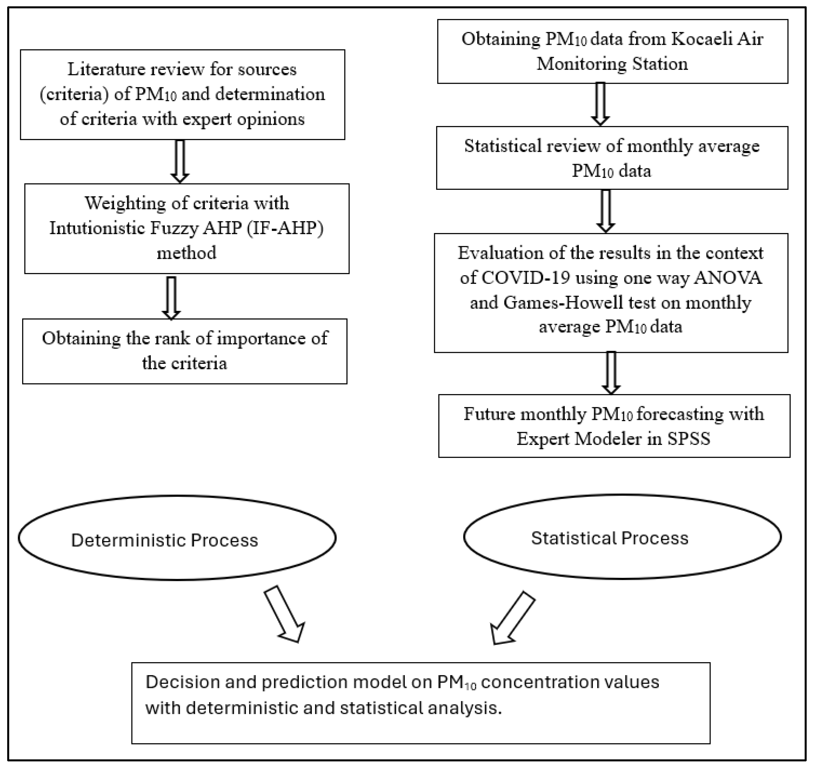
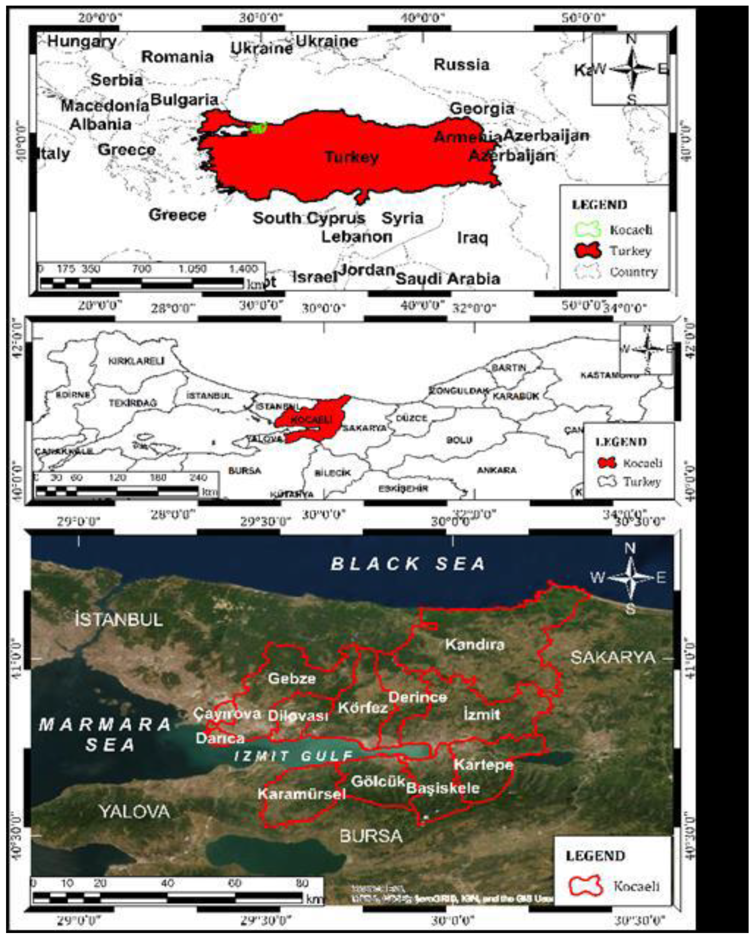
• As stated in the flowchart given in Figure 1, the study aimed to propose a decision model using deterministic and statistical analyses. For deterministic analysis, the criteria affecting PM₁₀ concentration values in Kocaeli city center are determined from a literature review and decision-makers’ opinions. The IF-AHP method is used for criterion weighting. The purpose of determining criterion weights with IF-AHP logic in the evaluation of criteria affecting PM₁₀ concentration values on a regional basis stems from the nature of the decision problem. The degree of hesitation is important for such intuitive decisions. According to the results obtained with IF-AHP, the most important criterion is determined to be C2: density of industrial facilities. The criterion that has the least impact on PM₁₀ concentration values is C1: adverse meteorological conditions.
• In the statistical analysis part of the study, PM₁₀ concentration values between 2017 and 2023, covering the pandemic period, are examined. Although significant decreases in air pollutant levels are observed in Europe and other regions during the pandemic period, these changes are not permanent as a result of the decrease in outdoor activities, transportation, and even industrial activities due to quarantine and restriction periods. Looking at the center of Kocaeli, the highest annual average PM₁₀ concentration value was recorded in 2018, when pandemic-related restrictions had not yet occurred. PM₁₀ concentration values started to increase significantly in 2020, 2021, and 2022. This increase may be an indication that heavy restrictions and measures are starting to lose their effectiveness. When this situation is associated with the results obtained using IF-AHP, effects such as remote working decisions or production restrictions in industrial facilities may have caused changes. Surprisingly, the monthly average concentration value reached its lowest level in 2023. The impact of this situation can be shown as the impact of economic pressure on industrial centers, but it may also be related to the adoption of some measures developed in 2023. The COVID-19 period quickly became permanent. Looking at the one-way ANOVA test results, there is a significant difference between the monthly average PM₁₀ concentration values for the years. Accordingly, it can be said that the harmful effects of air pollution and PM₁₀ in 2022 will be similar to the monthly average levels in 2019. The results obtained with the Games–Howell test valid for groups without variance homogeneity are given in Table A1 in Appendix A. According to Table A1 in Appendix A, considering that 2020 is the most critical year for COVID-19, there are significant differences between the years before 2020 and those after 2020. In this context, it is important to base the forecast on the period after 2020 for the sake of accuracy.
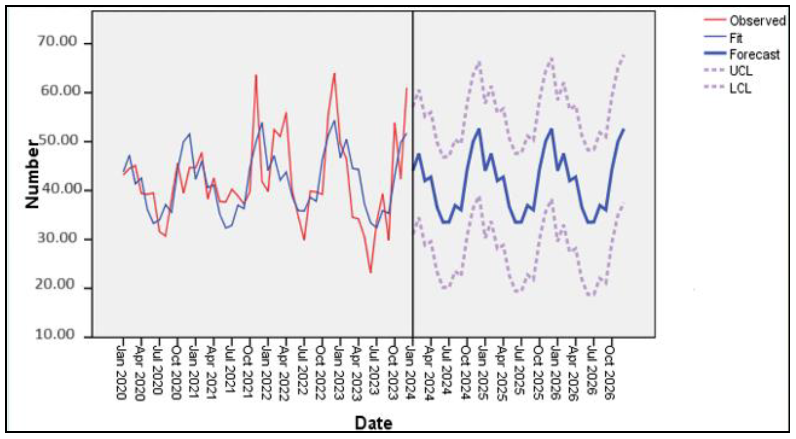
• In this study, monthly average PM₁₀ values in 2020–2023 are estimated with the Expert Modeler tool in the software IBM^® SPSS^® Statistics version 22. The Expert Modeler tool determined the most appropriate forecasting model to be the simple seasonal model. Using the model data, 36-month estimated PM₁₀ concentration values for 2024–2026 were obtained (Table A2 in Appendix A). In checking the estimated values obtained, the criterion weights obtained with IF-AHP can be examined by policymakers and decision-makers, and this examination may pave the way for more detailed analyses in future studies.

The motivation and innovation part of this study is that it can provide some inferences to decision-makers and managers with a statistical and deterministic MCDM approach specifically for PM₁₀ particulate matter.

References

1. Du, M.; Liu, W.; Hao, Y. Spatial correlation of air pollution and its causes in Northeast China. Int. J. Environ. Res. Public Health 2021, 18, 10619. [Google Scholar] [CrossRef]
2. Güzel, Ş.; Özer, P. Türkiye’de hava kirliliği ve sağlık harcamaları. Sağlık Ve Sos. Refah Araştırmaları Derg. 2022, 4, 186–202. [Google Scholar] [CrossRef]
3. California Air Resources Board “Inhalable Particulate Matter and Health (PM2.5 and PM10)”. Available online: https://ww2.arb.ca.gov/resources/inhalable-particulate-matter-and-health (accessed on 19 July 2024).
4. US EPA. America’s Children and the Environment; EPA: Washington, DC, USA, 2013.
5. Türkiye Environmental Problems and Priorities Assessment Report. Available online: https://webdosya.csb.gov.tr/db/ced/icerikler/turk-ye-cevre-sorunlari-ve-oncel-kler-_2022_3_ver3.logoduzenlendi-20230901135641.pdf (accessed on 21 April 2024).
6. WHO. Available online: https://iris.who.int/handle/10665/345329 (accessed on 29 May 2024).
7. European Environment Agency. Available online: https://www.eea.europa.eu/publications/status-of-air-quality-in-Europe-2022/europes-air-quality-status-2022/world-health-organization-who-air (accessed on 4 May 2024).
8. Vural, E.; Şahinalp, M.S. Investigation of particulate matter pollution in Şanlıurfa city under the influence of topographic and climatic factor. Turk. Geogr. Rev. 2023, 84, 53–66. [Google Scholar] [CrossRef]
9. Cetin, M.; Onac, A.K.; Sevik, H.; Sen, B. Temporal and regional change of some air pollution parameters in Bursa. Air Qual. Atmos. Health 2019, 12, 311–316. [Google Scholar] [CrossRef]
10. Aydınoğlu, A.Ç.; Bovkır, R.; Bulut, M. Geographical big data management and analysis in smart cities: The example of air quality. J. Geomat. 2022, 7, 174–186. [Google Scholar] [CrossRef]
11. Eroğlu, İ. Çerkezköy ve Kapaklı ilçelerinde (Tekirdağ) hava kirliliğinin nedenleri ve kirlilik parametreleri üzerine bir değerlendirme. J. Soc. Sci. 2023, 66, 256–283. [Google Scholar]
12. Birim, N.G.; Turhan, C.; Atalay, A.S.; Akkurt, G.G. The influence of meteorological parameters on PM10: A statistical analysis of an urban and rural environment in Izmir/Türkiye. Atmosphere 2023, 14, 421. [Google Scholar] [CrossRef]
13. Zajusz-Zubek, E.; Mainka, A.; Kaczmarek, K. Dendrograms, heat maps and principal component analysis—The practical use of statistical methods for source apportionment of trace elements in PM10. J. Environ. Sci. Health Part A 2023, 58, 163–170. [Google Scholar] [CrossRef] [PubMed]
14. Ul-Saufie, A.Z.; Hamzan, N.H.; Zahari, Z.; Shaziayani, W.N.; Noor, N.M.; Zainol, M.R.R.M.A.; Sandu, A.V.; Deak, G.; Vizureanu, P. Improving air pollution prediction modelling using wrapper feature selection. Sustainability 2022, 14, 11403. [Google Scholar] [CrossRef]
15. Erener, A.; Sarp, G.; Yıldırım, Ö. Seasonal air pollution investigation and relation analysis of air pollution parameters to meteorological data (Kocaeli/Türkiye). In Advances in Remote Sensing and Geo Informatics Applications, 4th ed.; El-Askary, H.M., Lee, S., Heggy, E., Pradhan, B., Eds.; Springer: Cham, Switzerland, 2019; pp. 355–358. [Google Scholar]
16. Bai, L.; Jiang, L.; Yang, D.-Y.; Liu, Y.-B. Quantifying the spatial heterogeneity influences of natural and socioeconomic factors and their interactions on air pollution using the geographical detector method: A case study of the Yangtze River Economic Belt, China. J. Clean. Prod. 2019, 232, 692–704. [Google Scholar] [CrossRef]
17. Li, L.; Qian, J.; Ou, C.-Q.; Zhou, Y.-X.; Guo, C.; Guo, Y. Spatial and temporal analysis of air pollution index and its timescale-dependent relationship with meteorological factors in Guangzhou, China, 2001–2011. Environ. Pollut. 2014, 190, 75–81. [Google Scholar] [CrossRef]
18. Lu, D.; Xu, J.; Yang, D.; Zhao, J. Spatio-temporal variation and influence factors of PM2.5 concentrations in China from 1998 to 2014. Atmos. Pollut. Res. 2017, 8, 1151–1159. [Google Scholar] [CrossRef]
19. Jiang, L.; Zhou, H.-F.; Bai, L.; Zhou, P. Does foreign direct investment drive environmental degradation in China? An empirical study based on air quality index from a spatial perspective. J. Clean. Prod. 2018, 176, 864–872. [Google Scholar] [CrossRef]
20. Lin, X.; Wang, D. Spatiotemporal evolution of urban air quality and socioeconomic driving forces in China. J. Geogr. Sci. 2016, 26, 1533–1549. [Google Scholar] [CrossRef]
21. Kotan, B.; Erener, A. Seasonal forecasting of PM10, SO2 air pollutants with multiple linear regression and artificial neural networks. Geomatik 2023, 8, 163–179. [Google Scholar] [CrossRef]
22. Maleki, H.; Sorooshian, A.; Goudarzi, G.; Baboli, Z.; Birgani, Y.T.; Rahmati, M. Air pollution prediction by using an artificial neural network model. Clean Technol. Environ. Policy 2019, 21, 1341–1352. [Google Scholar] [CrossRef] [PubMed]
23. Yadav, V.; Nath, S. Novel Application of Artificial Neural Network Techniques for Prediction of Air Pollutants Using Stochastic Variables for Health Monitoring: A Review. In Soft Computing in Condition Monitoring and Diagnostics of Electrical and Mechanical Systems: Novel Methods for Condition Monitoring and Diagnostics, 3rd ed.; Malik, H., Iqbal, A., Yadav, A.K., Eds.; Springer: Singapore, 2020; pp. 231–245. [Google Scholar]
24. Dutta, A.; Jinsart, W. Air pollution in Indian cities and comparison of MLR, ANN and CART models for predicting PM10 concentrations in Guwahati, India. Asian J. Atmos. Environ. 2021, 15, 2020131. [Google Scholar] [CrossRef]
25. Yılmaz, Z.; Karagözoğlu, M.B. Evaluation of Air Pollution (PM10 And SO2) by Anova Method–The Case Of Mardin (Türkiye) Province. Kirklareli Univ. J. Eng. Sci. 2022, 8, 343–356. [Google Scholar]
26. Huang, C.-Y.; Chung, P.-H.; Shyu, J.Z.; Ho, Y.-H.; Wu, C.-H.; Lee, M.-C.; Wu, M.-J. Evaluation and selection of materials for particulate matter MEMS sensors by using hybrid MCDM methods. Sustainability 2018, 10, 3451. [Google Scholar] [CrossRef]
27. Kokaraki, N.; Hopfe, C.J.; Robinson, E.; Nikolaidou, E. Testing the reliability of deterministic multi-criteria decision-making methods using building performance simulation. Renew. Sustain. Energy Rev. 2019, 112, 991–1007. [Google Scholar] [CrossRef]
28. Triantaphyllou, E.; Sánchez, A. A sensitivity analysis approach for some deterministic multi-criteria decision-making methods. Decis. Sci. 1997, 28, 151–194. [Google Scholar] [CrossRef]
29. de Moraes, L.B.; Parpinelli, R.S.; Fiorese, A. Application of deterministic, stochastic, and hybrid methods for cloud provider selection. J. Cloud Comput. 2022, 11, 5. [Google Scholar] [CrossRef]
30. Dutheil, F.; Baker, J.S.; Navel, V. COVID-19 as a Factor Influencing Air Pollution? Environ. Pollut. 2020, 263, 114466. [Google Scholar] [CrossRef] [PubMed]
31. McCann, J.E.; Zajchowski, C.A.B.; Hill, E.L.; Zhu, X. Air Pollution and Outdoor Recreation on Urban Trails: A Case Study of the Elizabeth River Trail, Norfolk. Atmosphere 2021, 12, 1304. [Google Scholar] [CrossRef]
32. Pepe, E.; Bajardi, P.; Gauvin, L.; Privitera, F.; Lake, B.; Cattuto, C.; Tizzoni, M. COVID-19 outbreak response, a dataset to assess mobility changes in Italy following national lockdown. Sci. Data 2020, 7, 230. [Google Scholar] [CrossRef] [PubMed]
33. Galeazzi, A.; Cinelli, M.; Bonaccorsi, G.; Pierri, F.; Schmidt, A.L.; Scala, A.; Pammolli, F.; Quattrociocchi, W. Human Mobility in Response to COVID-19 in France, Italy and UK. Sci. Rep. 2021, 11, 13141. [Google Scholar] [CrossRef] [PubMed]
34. Menut, L.; Bessagnet, B.; Siour, G.; Mailler, S.; Pennel, R.; Cholakian, A. Impact of Lockdown Measures to Combat COVID-19 on Air Quality Over Western Europe. Sci. Total. Environ. 2020, 741, 140426. [Google Scholar] [CrossRef]
35. TURKSTAT. Available online: https://cip.tuik.gov.tr/ (accessed on 2 April 2024).
36. Kotan, B.; Erener, A. Seasonal analysis and mapping of air pollution (PM10 and SO2) during Covid-19 lockdown in Kocaeli (Türkiye). Int. J. Eng. Geosci. 2023, 8, 173–187. [Google Scholar] [CrossRef]
37. National Air Quality Monitoring Network (Naqmn). Available online: https://www.bafu.admin.ch/bafu/en/home/topics/air/state/data/national-air-pollution-monitoring-network--nabel-.html (accessed on 10 April 2024).
38. Mayyas, A.; Shen, Q.; Mayyas, A.; Abdelhamid, M.; Shan, D.; Qattawi, A.; Omar, M. Using quality function deployment and analytical hierarchy process for material selection of body-in-white. Mater. Des. 2011, 32, 2771–2782. [Google Scholar] [CrossRef]
39. Laarhoven, P.J.; Pedrycz, W. A fuzzy extension of Saaty’s priority theory. Fuzzy Sets Syst. 1983, 11, 229–241. [Google Scholar] [CrossRef]
40. Buckley, J.J.; Uppuluri, V.R.R. Fuzzy hierarchical analysis. In Uncertainty in Risk Assessment, Risk Management, and Decision Making; Springer: Boston, MA, USA, 1985; pp. 389–401. [Google Scholar]
41. Chang, D.-Y. Applications of the extent analysis method on fuzzy AHP. Eur. J. Oper. Res. 1996, 95, 649–655. [Google Scholar] [CrossRef]
42. Abdullah, L.; Najib, L. A new type-2 fuzzy set of linguistic variables for the fuzzy analytic hierarchy process. Expert Syst. Appl. 2014, 41, 3297–3305. [Google Scholar] [CrossRef]
43. Boran, F.E.; Genç, S.; Kurt, M.; Akay, D. A multi-criteria intuitionistic fuzzy group decision making for supplier selection with TOPSIS method. Expert Syst. Appl. 2009, 36, 11363–11368. [Google Scholar] [CrossRef]
44. Xu, Z. Intuitionistic fuzzy aggregation operators. IEEE Trans. Fuzzy Syst. 2007, 15, 1179–1187. [Google Scholar] [CrossRef]
45. Saaty, T.L. How to make decision: The Analytic Hierarchy Process. Eur. J. Oper. Res. 1990, 48, 9–26. [Google Scholar] [CrossRef]
46. Brown, A.M. A new software for carrying out one-way ANOVA post hoc tests. Comput. Methods Programs Biomed. 2005, 79, 89–95. [Google Scholar] [CrossRef]
47. Victor, C.C.; Confidence, I.N.; Frederick, A.O.; Chukwuenyem, E.O. Forecasting the Rainfall of Anambra State using Timeseries Model. Int. J. Trend Sci. Res. Dev. 2024, 8, 1056–1060. [Google Scholar]
48. IBM. Available online: https://www.ibm.com/docs/tr/spss-statistics/29.0.0?topic=modeler-specifying-options-expert (accessed on 12 May 2024).
49. Kendre, V.; Dixit, J.V.; Bahattare, V.N.; Wadagale, A.V. Forecasting measles vaccine requirement by using time series analysis. J. Evol. Med. Dent. Sc. 2017, 6, 2329–2333. [Google Scholar] [CrossRef]
50. Pawar, S.D.; Kore, M.; Athalye, A.; Thombre, P. Seasonality of leptospirosis and its association with rainfall and humidity in Ratnagiri, Maharashtra. Int. J. Health Allied Sci. 2018, 7, 37–40. [Google Scholar] [CrossRef]
51. Ma, E.; Za, M.A.; Ar, J. Forecasting Malaysia COVID-19 incidence based on movement control order using ARIMA and expert modeler. IIUM Med. J. Malays. 2020, 19, 1–8. [Google Scholar] [CrossRef]
52. Gülkesen, S. Covid-19 Süresinde Ruh Sağlığı İle İlgili İçeriklerin İnternette Aranma Eğilimi: Google Trends Analizi. Unpublished. Master’s Thesis, Akdeniz University, Antalya, Türkiye, 2022. [Google Scholar]
53. Zerin, N.H.; Sayem, A.S.M. Prioritizing the Factors Influenced Particulate Matter Emission Applying Fuzzy Topsis. Mech. Eng. Res. J. 2022, 12, 30–40. [Google Scholar]
54. Shahid, I.; Kistler, M.; Mukhtar, A.; Ghauri, B.M.; Cruz, C.R.-S.; Bauer, H.; Puxbaum, H. Chemical characterization and mass closure of PM10 and PM2.5 at an urban site in Karachi—Pakistan. Atmos. Environ. 2016, 128, 114–123. [Google Scholar] [CrossRef]
55. Khanum, F.; Chaudhry, M.N.; Kumar, P. Characterization of five-year observation data of fine particulate matter in the metropolitan area of Lahore. Air Qual. Atmos. Health 2017, 10, 725–736. [Google Scholar] [CrossRef]
56. Ramanathan, V.; Carmichael, G. Global and regional climate changes due to black carbon. Nat. Geosci. 2008, 1, 221–227. [Google Scholar] [CrossRef]
57. Begum, B.A.; Saroar, G.; Nasiruddin, M.; Randal, S.; Sivertsen, B.; Hopke, P.K. Particulate matter and Black Carbon monitoring at urban environment in Bangladesh. Nucl. Sci. Appl. 2014, 23, 21–28. [Google Scholar]
58. Clifford, A.; Lang, L.; Chen, R.; Anstey, K.J.; Seaton, A. Exposure to air pollution and cognitive functioning across the life course—A systematic literature review. Environ. Res. 2016, 147, 383–398. [Google Scholar] [CrossRef] [PubMed]
59. Cohen, A.J.; Brauer, M.; Burnett, R.; Anderson, H.R.; Frostad, J.; Estep, K.; Balakrishnan, K.; Brunekreef, B.; Dandona, L.; Dandona, R.; et al. Estimates and 25-year trends of the global burden of disease attributable to ambient air pollution: An analysis of data from the Global Burden of Diseases Study 2015. Lancet 2017, 389, 1907–1918. [Google Scholar] [CrossRef]
60. İlten, N.; Selici, T. Investigating the Impacts of Some Meteorological Parameters on Air Pollution in Balikesir, Türkiye. Environ. Monit. Assess. 2008, 140, 267–277. [Google Scholar] [CrossRef]
61. Keser, N. Kütahya’da Hava Kirliliğine Etki Eden Topografik ve Klimatik Faktörler. Marmara Coğrafya Derg. 2002, 5, 69–100. [Google Scholar]
62. Menteşe, S.; Tağıl, Ş. Bilecik’te iklim elemanlarının hava kirliliği üzerine etkisi. Balıkesir Üniversitesi Sos. Bilim. Enstitüsü Derg. 2012, 15, 3–16. [Google Scholar]
63. Ilıc, I.Z.; Dragana, T.Z.; Nenad, M.V.; Dejan, M.B. Investigation of the Correlation Dependence Between SO2 Emission Concentration and Meteorological Parameters: Case Study—Bor (Serbia). J. Environ. Sci. Health 2010, 45, 901–907. [Google Scholar] [CrossRef]
64. Akyürek, Ö.; Arslan, O.; Karademir, A. SO2 ve PM10 hava kirliliği parametrelerinin CBS ile konumsal analizi: Kocaeli örneği. In Proceedings of the TMMOB Coğrafi Bilgi Sistemleri Kongresi, Ankara, Türkiye, 11–13 November 2013. [Google Scholar]
65. T.C. Uskudar University. Available online: https://uskudar.edu.tr/tr/icerik/6852/hizli-nufus-artisi-dogal-cevreyi-olumsuz-etkiliyor (accessed on 8 April 2024).
66. Gürbüz, H.; Gürdal, H.A.; Durmuş, H. Partiküler Madde (PM10) Miktarına Etki Eden Faktörlerin Belirlenmesi: Eskişehir İl Merkezi Örneği. In Proceedings of the 9th World Conference of Business Economics Management, Porto, Portugal, 1–3 October 2020. [Google Scholar]
67. Bilgili, M.S.; Demir, A.; Varank, G. Evaluation and modeling of biochemical methane potential (BMP) of landfilled solid waste: A pilot scale study. Bioresour. Technol. 2009, 100, 4976–4980. [Google Scholar] [CrossRef] [PubMed]
68. Batur, A.; Aksu, G.A. Partikül madde (PM10) konsantrasyonunun kentsel yeşil alan sisteminin değerlendirilmesinde ekolojik İndikatör olarak kullanımı: İstanbul-Beşiktaş örneği. Avrupa Bilim Ve Teknol. Derg. 2021, 27, 125–134. [Google Scholar] [CrossRef]
69. Kopar, İ.; Zengin, M. Coğrafi faktörlere bağlı olarak Erzurum kentinde hava kalitesinin zamansal ve mekansal değişiminin belirlenmesi. Türk Coğrafya Derg. 2009, 53, 51–68. [Google Scholar]
70. Tağıl, Ş. Balıkesir’de hava kirliliğinin solunum yolu hastalıklarının mekânsal dağılımı üzerine etkisini anlamada jeo-istatistik teknikler. Coğrafi Bilim. Derg. 2007, 5, 37–56. [Google Scholar]
71. Menteşe, S.; Tağıl, Ş. Topografyanın Hava Kirliliği Üzerindeki Etkisi: Zonguldak Örneği. In Proceedings of the Türkiye Coğrafyası Araştırma ve Uygulama Merkezi VII, Coğrafya Sempozyumu, Ankara, Türkiye, 23–24 October 2014. [Google Scholar]
72. Rai, A.; Chakrabarty, P.; Sarkar, A. Forecasting the demand for medical tourism in India. IOSR J. Humanit. Soc. Sci. 2014, 19, 22–30. [Google Scholar] [CrossRef]
73. Masum, M.H.; Pal, S.K. Statistical evaluation of selected air quality parameters influenced by COVID-19 lockdown. Glob. J. Environ. Sci. Manag. 2020, 6, 85–94. [Google Scholar]
74. Kirkitadze, D.D. Statistical Characteristics of Monthly Mean and Annual Concentrations of Particulate Matter PM2.5 and PM10 in Three Points of Tbilisi in 2017–2022. J. Georgian Geophys. Soc. 2023, 26, 67–82. [Google Scholar] [CrossRef]
75. Cabello-Torres, R.J.; Estela, M.A.P.; Sánchez-Ccoyllo, O.; Romero-Cabello, E.A.; Ávila, F.F.G.; Castañeda-Olivera, C.A.; Valdiviezo-Gonzales, L.; Eulogio, C.E.Q.; De La Cruz, A.R.H.; López-Gonzales, J.L. Statistical modeling approach for PM10 prediction before and during confinement by COVID-19 in South Lima, Perú. Sci. Rep. Inst. 2022, 12, 16737. [Google Scholar] [CrossRef]
76. Zoran, M.A.; Savastru, R.S.; Savastru, D.M.; Tautan, M.N. Assessing the relationship between surface levels of PM2.5 and PM10 particulate matter impact on COVID-19 in Milan, Italy. Sci. Total. Environ. 2020, 738, 139825. [Google Scholar] [CrossRef]
77. Kurnaz, G.; Demir, A.S. Prediction of SO2 and PM10 air pollutants using a deep learning-based recurrent neural network: Case of industrial city Sakarya. Urban Clim. 2022, 41, 101051. [Google Scholar] [CrossRef]
78. Zeydan, Ö; Pekkaya, M. Evaluating air quality monitoring stations in Turkey by using multi criteria decision making. Atmos. Pollut. Res. 2021, 12, 101046. [Google Scholar] [CrossRef]
79. Hadi-Vencheh, A.; Tan, Y.; Wanke, P.; Loghmanian, S.M. Air pollution assessment in China: A novel group multiple criteria decision making model under uncertain information. Sustainability 2021, 13, 1686. [Google Scholar] [CrossRef]
80. Chauhan, A.; Jariwala, N.; Christian, R.A. Comparative approach to spatial and temporal prioritization of the criteria air pollutants using different multi-criteria decision-making methods in urban context. In AIP Conference Proceedings; AIP Publishing: Canberra, Australia, 2023; Volume 2855. [Google Scholar]
Figure 1. Flow diagram of this study’s process.
Sustainability 16 07851 g001
Figure 2. Location of Kocaeli on the map of Türkiye [36].
Sustainability 16 07851 g002
Figure 3. Kocaeli air quality monitoring station (central).
Sustainability 16 07851 g003
Figure 4. Expert Modeler interface in IBM® SPSS® Statistics 22 software.
Sustainability 16 07851 g004
Figure 5. Graphical view of the estimated PM10 concentration values.
Sustainability 16 07851 g005