Employment Quality and Migration Intentions: A New Perspective from China’s New-Generation Migrant Workers

Abstract

This study explores the factors influencing the migration intentions of the new generation of migrant workers from the perspective of employment quality. Utilizing differential analysis, correlation analysis, and the Partial Least Squares Structural Equation Modeling (PLS-SEM) model, this study analyzes data on hukou transfer intention obtained through an exploratory questionnaire survey. The results indicate significant differences in migration intentions among new-generation migrant workers differentiated by job industry, job position, gender, household registration type, and housing type. Additionally, age, the number of local family members, and housing satisfaction are strongly correlated with migration intentions. Path analysis reveals that employment stability, income–expenditure match, and social integration significantly positively affect migration intentions. This research provides a unique perspective on employment quality and offers theoretical foundations for policies related to migrant workers’ hukou transfer intention.

1. Introduction

China has been committed to fostering urban–rural integration and new urbanization initiatives. However, as the urbanization process continues, the migration of the rural population into urban areas has shown signs of slowing down and lacking momentum. According to the latest official statistics, in 2023, the total number of migrant workers in China was approximately 297.53 million, of which 176.58 million were migrant workers living outside their hometowns, and by the end of the year, 128.16 million were residing in urban areas according to National Bureau of Statistics in 2023. The concept of “new generation migrant workers”, originating in sociology, refers to individuals born after 1980 from rural or urban backgrounds who primarily engage in non-agricultural jobs in places other than their hometowns according to National Bureau of Statistics in 2011. Their motivations for moving are increasingly based on personal development and limited social experience, showing distinct generational differences from those born before 1980. Despite significantly lowered barriers for migrant workers to settle in cities, the migration intentions of the new generation are generally lower than policy expectations. Guiding the integration of this population into urban settings in an efficient and orderly manner remains one of the major challenges for achieving high-quality economic development in China.

Hukou transfer intention is defined as the willingness of urban newcomers to give up their original rural or other city household registrations to relocate their household registrations to a new city [1,2]. Research on this topic has focused on four main areas: individual characteristics, family traits, urban attributes, and policy and institutional factors. Specifically, individual characteristics which have been investigated include age [3], life cycle stages [4], cultural level [5], type of household registration [6], education level [7,8], career mobility [9], duration of time spent outside one’s hometown [10], psychological perceptions [11], and income [12]. Family traits emphasize the role of social capital [13], particularly how social networks based on primary groups can restrict interactions. Urban attributes cover economic aspects such as disparities in economic development between origin and destination [14], urban housing prices, and industrial structures [15]. Non-economic aspects include the urban society, institutional and cultural factors [16], and the state of social integration in the destination [17]. Policy and institutional factors have been a recent focus, critically examining how registration systems, urban migration policies, rural land ownership policies, and social security create barriers to migration [18,19,20].

Employment quality encompasses not only the objective conditions related to work, such as wage income, employment stability, labor security, and labor intensity, but also the subjective psychological aspects experienced by workers, including job satisfaction and overall well-being [21]. Few studies have systematically examined the impact of employment quality on hukou transfer intentions. High-quality employment not only boosts income and reduces perceived risks, but also facilitates social integration with urban residents, building stable networks and enhancing a sense of belonging to the city, which ultimately influences migration decisions [22]. Moreover, with socio-economic advancements, the employment expectations of the new generation of migrant workers have risen, leading to higher demands for job quality and stability. Unlike their predecessors, this generation exhibits less job stability and a higher frequency of job changes, reflecting a shift from survival- to development-oriented employment motivations [23,24].

This study aims to analyze the factors influencing the hukou transfer intentions of migrant workers from the perspective of employment quality. Utilizing a large-scale questionnaire survey, this study gathers data on the migration intentions of frontline migrant workers. The study employs differential and correlational analyses and utilizes Partial Least Squares Structural Equation Modeling (PLS-SEM) to explore the impact of employment quality on migration intentions. This approach involves selecting latent variables, testing reliability and validity, and conducting path analysis. The findings provide a theoretical basis for policies related to migrant workers’ hukou transfer intention.

The innovations of this study are threefold: Firstly, it explores the issue of migration from the novel perspective of employment quality, adding to the existing body of research. In contrast to traditional research that relies on a single employment quality indicator to describe migration intention, this study takes a more comprehensive approach by examining employment quality through three dimensions: employment stability, income–expenditure match, and social integration. We explore how these three factors influence migrant workers’ hukou transfer intentions. This research contributes a novel employment quality perspective to the existing literature on migrant workers’ migration intentions, offering a more comprehensive understanding of the factors that influence these intentions. Secondly, the introduction of the PLS-SEM method in studying the relationship between employment quality and migration intentions is novel. Lastly, the data were collected via an online survey, capturing the latest intentions of migrant workers regarding hukou transfer intention.

The rest of the paper is organized as follows. The next chapter reviews literature related to employment quality and introduces the hypotheses of this study. Chapter three details the data collection methods and describes the PLS-SEM approach, including the modeling and estimation processes. Chapter four conducts differential and correlational analyses and empirical PLS-SEM analysis, followed by a discussion of the results. The paper concludes by summarizing the findings and proposing policy recommendations.

2. Literature Review and Research Hypotheses

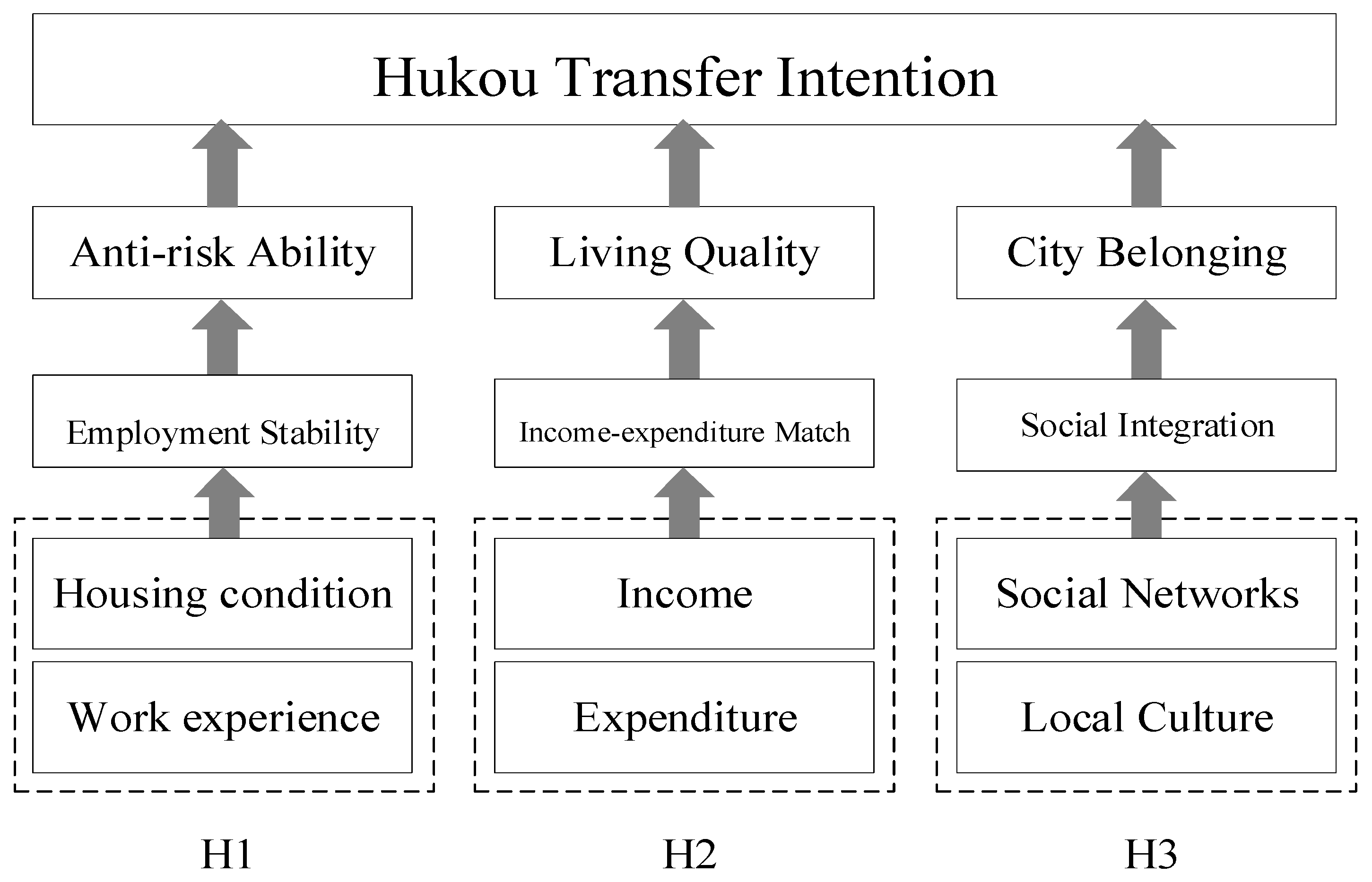
2.1. Impact of Employment Stability on Hukou Transfer Intention

The concept of employment stability can be understood from both macro and micro perspectives. From the macro perspective, employment stability refers to the ability of the labor force to maintain a certain level of participation over a significant period. This includes overall employment, the elasticity of labor movement between industries, and total individual employment duration from the micro perspective. The focus is on individual labor indicators, assessing whether a worker can maintain stable employment within a specific time frame [25]. In this study, employment stability is primarily measured from the micro perspective, utilizing individual work experience and housing conditions.

Employment stability is a crucial metric for assessing the employment quality of migrant workers and significantly impacts their hukou transfer intentions. Stable employment enables migrant workers to integrate and settle in cities, which is central to new urbanization efforts. However, the literature shows divergent views on the impact of employment stability on migrant workers’ intentions to settle in cities. The prevailing opinion, based on new economic migration theories, suggests that employment stability positively affects migration intentions [26], aligning with findings from international studies on immigration [27]. High employment stability helps migrant workers integrate into urban social networks and strengthens their sense of belonging to the city [28]. It also improves migrant workers’ employment income and ensures an economic basis for urban settlement [29].

Conversely, some studies argue that higher employment stability may insignificantly or negatively impact the desire to settle in cities. Higher stability could reduce opportunities for social and psychological integration within the city, thus lowering the hukou transfer intentions [30] or diminishing its positive effects [31]. Furthermore, employment stability could increase the likelihood of deprivation in terms of working hours, income level, and social security, reducing the sense of urban belonging [32] and adversely affecting migration intentions.

This study posits that, for migrant workers with high employment stability, the uncertainty regarding future employment quality is lower, and their ability to handle uncertainties after migrating their registration is stronger, leading to higher intention to migrate. Employment stability is divided into two latent variables in

Table 1. Employment stability variable table.

Primary Construct	Secondary Construct	Indicator	Reference
Employment stability	Housing condition	Housing type	[33,34]
		Housing size	[35,36]
		Housing satisfaction	[37,38]
		Commuting time	[39,40]
		Household registration type	[41,42]
	Work experience	Work seniority	[43,44]
		Age	[45,46]
		Job position	[47,48]
		Years lived locally	[10,49]
		Job change frequency	[9,50]

: housing conditions and work experience. Based on this, Hypothesis 1 of this paper is:

H1. 

Higher employment stability increases the hukou transfer intention.

2.2. Impact of Income–Expenditure Match on Hukou Transfer Intention

Income–expenditure match refers to the degree to which an individual’s actual income aligns with their expenditures over a specific period, such as a month, a quarter, or a year [51]. It reflects the efficiency and stability of an individual’s financial management and is a crucial indicator of their economic condition. It also significantly influences the intentions to migrate household registration, primarily assessing whether their current income can meet normal living expenses. A high degree of income–expenditure match enhances life quality and reduces social stress, thereby positively impacting migration intentions [52].

The literature suggests that during industrialization, due to wage disparities between traditional agricultural sectors and modern sectors, rural surplus labor earning lower incomes in traditional sectors can achieve higher wages upon moving to modern sectors [53]. A high income–expenditure match can effectively improve living quality and significantly promote hukou transfer intention [54,55]. Moreover, the balance between employment income and living expenses influences migration intentions and urbanization trends [56], making the inclusion of both employment income and living expenses in the assessment more scientifically robust than traditional studies focusing solely on income levels.

This study posits that migrant worker families with favorable income–expenditure situations are better able to afford the increased living costs after migrating their registration, thus displaying a higher intention to migrate. In

Table 2. Income–expenditure match variable table.

Primary-Construct	Secondary-Construct	Indicator	Reference
Income–expenditure match	Income	Annual personal income	[12,57]
		Annual family income	[58,59]
		Job industry	[60,61]
		Economic level	[20,62]
	Expenditure	Housing expenditure	[63,64]

, the designed latent variables include factors such as income, expenditure, and employment sectors. We estimate the impacts of varying income–expenditure situations on migration intentions. Based on this, Hypothesis 2 of this paper is:

H2. 

A higher income–expenditure match increases the hukou transfer intention.

2.3. Impact of Social Integration on Hukou Transfer Intention

While economic factors play a crucial role in the initial decision of rural laborers to migrate, for migrant workers who have already settled in cities, the decision to pursue permanent migration is more significantly influenced by sociocultural factors [65]. Over time, migrant workers tend to adapt to urban life at a psychological level, developing a strong sense of identity and belonging, which fosters full integration into city life. The ability of migrant workers to adapt to the economic, social, cultural, and psychological aspects of urban living is not only a critical consideration in their decision to migrate permanently, but also a pressing issue with significant implications for the urbanization process in China [66].

Social integration is a comprehensive concept that encompasses economic, social, psychological, and identity integration [67]. In this study, social integration primarily focuses on the participation of migrant workers in urban social networks and their acceptance of local culture. The state of social integration significantly influences their intentions to migrate household registration, as differences in social networks and cultural backgrounds between urban and rural areas often play a crucial role in their decision-making processes.

Studies suggest that active engagement in social networks can enhance migrant workers’ senses of identity and happiness, improving their quality-of-life assessments and ultimately fostering their willingness to settle in their destination [68,69]. The degree of cultural acceptance can sometimes have a more significant impact on migration intentions than economic factors, becoming a primary criterion for deciding whether to migrate [70].

This study posits that high levels of social integration increase migrant workers’ senses of belonging and identification with the city, positively influencing their migration intentions. In

Table 3. Social integration variable table.

Primary-Construct	Secondary-Construct	Indicator	Reference
Social integration	Participation of social networks	Local friends	[71,72]
		Friends with local household registration	[7,73]
		Friends without local household registration	[74,75]
		social activities	[76,77]
	Acceptance of local culture	Local identity	[61,78]
		Cultural and customary identity	[79,80]

, by constructing latent variables for social integration and incorporating observational variables such as frequency of participation in social activities, number of local friends, and degree of cultural norm acceptance, the model integrates aspects of social network participation and cultural acceptance. Based on this, Hypothesis 3 of this paper is:

H3. 

Higher social integration increases the hukou transfer intention.

The overall framework of this study is summarized in Figure 1.

3. Data and Research Methods

3.1. Data Collection

This survey was conducted from 2 February 2024 to 9 April 2024. The online questionnaire was designed through the platform of WenJuanXing, a leading consultancy in China, and distributed via the WeChat platform. The respondents were identified as new-generation migrant workers if they were born after 1980 and had been working in the locality for more than 6 months without local hukou. The response rate, which measures the percentage of participants who answer all questions, was used to gauge the overall engagement of the participants [81]. Generally, a response rate of 70% or higher is generally considered positive, providing a reliable foundation for further research. In this study, 201 questionnaires were distributed online, and 195 valid responses were received, resulting in a 97.01% response rate. These samples cover more than ten provinces in China, with Beijing having the largest number of samples, accounting for 42.56%. The rest of the samples are also from cities with high concentrations of migrant workers in China, such as Nanjing, Shanghai, Shenzhen, Suzhou, and Tianjin.

3.2. Ethics Statement

In this study, the respondents were informed of the purpose of this questionnaire in writing at the beginning of the questionnaire. All respondents participated voluntarily, and there were no minors.

3.3. Partial Least Squares Structural Equation Model (PLS-SEM)

3.3.1. Introduction of PLS-SEM Method

Partial Least Squares Structural Equation Modeling (PLS-SEM), developed by Swedish economist Wold [82,83], is designed to efficiently model complex structures involving multiple indicator variables and structural paths [84,85]. PLS-SEM combines principal component analysis with multiple regression to provide causal explanations and predictive power in estimating statistical models [83,86,87].

Compared to traditional covariance-based structural equation modeling (CB-SEM), PLS-SEM offers several advantages: (1) It does not require the assumption of data normality, making it applicable to a broader range of scenarios [88,89]. (2) It has more lenient sample size requirements, allowing for complex structural modeling even with small samples [90,91]. (3) PLS-SEM is particularly suitable for exploratory research on secondary data, such as company databases, media data, customer tracking data, official statistics, or publicly available survey data [2,84,89]. (4) It excels in identifying potential relationships between variables and is effective in testing emerging or underdeveloped theories [92,93]. (5) PLS-SEM achieves a higher degree of fit, enabling more accurate predictions [84]. The PLS-SEM has been increasingly applied in social science fields such as user satisfaction research [94], information management system evaluation [95], marketing management [96], supply chain management [97], hospitality management [98], and environmental research [99].

3.3.2. The Structure of PLS-SEM

PLS-SEM consists of a measurement model and a construct model. The detailed introductions of the measurement model and construct model are as follows.

(1)

Measurement model

A measurement model is used to reflect the relationship between a certain latent variable and its corresponding manifest variables. Suppose there are $J$ groups of manifest variables, and each group contains the $p_j$ variable. Then, each group of manifest variables can be expressed as follows: $X_j=\left(x_{j1},x_{j2},\cdots ,x_{j{p}_j}\right)\left(j=1,2,\cdots ,J\right)$. It is usually assumed that the manifest variables $X_j$ are based on $n$ common observations and that each manifest variable $x_{jh}\left(j=1,2,\cdots ,J;h=1,2,\cdots ,p_j\right)$ is centralized. Each set of manifest variables corresponds to a latent variable ${\xi }_j\left(j=1,2,\cdots ,J\right)$, which is assumed to be standardized. A measurement model is thereby formed between each set of manifest variables $X_j$ and the corresponding latent variable ${\xi }_j$.

The measurement model usually takes two modes. One is the reflective mode, which considers that the manifest variables are influenced by the latent variable. The relationship between $x_{jh}$ and ${\xi }_j$ is represented by the following linear equation.

$$x_{jh}={\lambda }_{jh}{\xi }_j+{\epsilon }_{jh},$$

(1)

where ${\lambda }_{jh}$ is the marginal intensity of the effect of j-th latent variable ${\xi }_j$ on its h-th manifest variable $x_{jh}$, named the loading coefficient. ${\epsilon }_{jh}$ is the random error term. Equation (1) requires the following assumption.

$$E\left(x_{jh}|{\xi }_j\right)={\lambda }_{jh}{\xi }_j,$$

(2)

which shows that ${\epsilon }_{jh}$ has a zero mean and is not correlated with ${\xi }_j$.

In reflective mode, a set of manifest variables $X_j$ can only reflect the characteristic of a single aspect of a thing, i.e., the latent variable ${\xi }_j$, reflected by $X_j$, is unique. The $X_j$ satisfying the above assumptions is considered to be unidimensional. Three commonly used methods for testing unidimensionality are: (1) Principal Component Analysis: the first eigenvalue of the correlation coefficient matrix of the observed variables is much larger than the other eigenvalues; (2) Cronbach’s alpha coefficient is greater than 0.7; (3) Dillion–Goldstein’s is greater than 0.7. When $X_j$ does not satisfy the unidimensionality test, some manifest variables should be deleted, or $X_j$ can be divided into several groups to satisfy the requirements.

Another kind of measurement model belongs to the formative mode. It considers that ${\xi }_j$ is determined by $X_j$. In such case, the model equation becomes

$${\xi }_j={\displaystyle \sum _{h=1}^{p_j}{w}_{jh}{x}_{jh}+{\delta }_j},$$

(3)

where $w_{jh}$ is the contribution intensity of $x_{jh}$ to ${\xi }_j$. ${\delta }_j$ is the random error term. Equation (3) should satisfy

$$E\left({\xi }_j|x_{j1},x_{j2},\cdots ,x_{jp}\right)={\displaystyle \sum _{h=1}^{p_j}{w}_{jh}{x}_{jh}},$$

(4)

which indicates that ${\delta }_j$ has a zero mean and is independent of $x_{jh}$.

(2)

Construct model

The construct model consisting of linear equations is used to describe the causal relationship between different latent variables with the following expressions.

$${\xi }_j={\displaystyle \sum _{i\ne j}{\beta }_{ji}{\xi }_i+}{\gamma }_j,$$

(5)

where ${\beta }_{ji}$ is the marginal intensity of the direct effect of ${\xi }_i$ on ${\xi }_j$. ${\beta }_{ji}$ is called the path coefficient. ${\gamma }_j$ is the random error, which has a zero mean and is not related to ${\xi }_j$.

3.3.3. The Estimation of PLS-SEM

The PLS-SEM model estimates the latent variables by iteration, which can be accomplished in two ways. One is to calculate the latent variable from the measurement model based on the relationship between the manifest variables and latent variable, called the external estimation. In this case, the latent variable can be estimated by a linear combination of the manifest variables, and the estimator is noted as $Y_j$. Since the latent variable is assumed to be standardized, there is

$$Y_j={\left({\displaystyle \sum _{h=1}^{p_j}{w}_{jh}{x}_{jh}}\right)}^{*}={\left(X_j{w}_j\right)}^{*},$$

(6)

where * denotes the operator of normalization of the estimated quantity.

Another way of estimating the latent variables is to start from the construct model and calculate according to the relationship between latent variables, which is called internal estimation. At this time, a certain latent variable is estimated by other latent variables, and denoting the estimator as $Z_j$, there is

$$Z_j={\left({\displaystyle \sum _{i:{\beta }_{ji}}{e}_{ji}{Y}_i}\right)}^{*},$$

(7)

where $e_{ji}$ is the internal weight, which represents the relationship between two latent variables linked by arrows in the construct model. There are three ways to set $e_{ji}$:

(1)

Factor weighting: $e_{ji}$ is equal to the correlation coefficient between $Y_j$ and $Y_i$, i.e.,

$$e_{ji}=corr(Y_j,Y_i).$$

(8)

(2)

Path weighting: All the latent variables connected with ${\xi }_j$ are divided into the premise (with arrow pointing to ${\xi }_j$) and the result (with arrow pointing out from ${\xi }_j$). For the premised latent variable ${\xi }_i$, $e_{ji}$ is equal to the regression coefficient in the linear regression of $Y_j$ against $Y_i$. And for the resulted latent variable ${\xi }_i$, $e_{ji}$ is equal to the correlation coefficient between $Y_j$ and $Y_i$.

(3)

Centroid method: $e_{ji}$ is equal to the sign function value of the correlation coefficient between $Y_j$ and $Y_i$, i.e.,

$$e_{ji}=sign\left(corr\left(Y_j,Y_i\right)\right)=\left\{\begin{array}{c}1, if corr\left(Y_j,Y_i\right)\ge 0\\ 0, if corr\left(Y_j,Y_i\right)<0\end{array}\right..$$

(9)

For the weight vector $w_j$ in Equation (6), there are two modes for estimation. Mode A has an expression of

$$w_j={\displaystyle \frac{1}{n}}{X}_j^T{Z}_j.$$

(10)

For standardized variables, $w_j$ is the correlation coefficient between the manifest variable cluster $X_j$ and the latent variable $Z_j$, which is actually equal to the first axis vector of the partial least squares regression for $Z_j$ against $X_j$.

Mode B has an expression of

$$w_j={\left(X_j^T{X}_j\right)}^{-1}{X}_j^T{Z}_j,$$

(11)

where $w_j$ is the regression coefficient of the ordinary least squares regression of the $Z_j$ against $X_j$.

Models A and B are applicable when the relationships between the manifest and latent variables are reflective and formative of patterns, respectively. The estimation error of Mode B is large because of the inevitable multicollinearity of the explicit variables in each group. It is more appropriate to use the partial least squares method of Model A to calculate the weights.

The iterative estimation process of the PLS-SEM for the latent variables is as follows, with the number of iterations denoted by $k$.

• Step 1: Given an arbitrary initial value of the weight vector $w_j^0$, $Y_j^0$ is calculated according to Equation (6).
• Step 2: Substitute $Y_j^0$ into Equation (7) to calculate $Z_j^0$. The internal weights can be set by choosing any one of Equations (8)–(10).
• Step 3: Re-estimate the external weight $w_j^1$ from Equation (10) or (11).
• Step 4: Repeat steps (1)–(3) until the preset maximum iterations are met, or stop when $\left|w_j^k-w_j^{k-1}<\epsilon \right|$ is satisfied. $\epsilon$ is the preset stop criterion. Finally, $Y_j^{k-1}$ is obtained as the estimated value of the latent variable ${\xi }_j$.
• Step 5: Based on $Y_j^{k-1}$, the coefficients ${\lambda }_{jh}$ (or $w_{jh}$) in the measurement model and ${\beta }_{ji}$ in the construct model are calculated using ordinary least squares estimation.

In this study, the measurement model belongs to reflective mode, the weighting scheme is set to path weighting, and the accuracy requirement is 10⁻⁷.

4. Results and Discussion

4.1. Demographic Characteristics and Differential Analysis

Frequency analysis of demographic variables showed that the survey included a total of 195 respondents in the survey. Specifically, (1) in terms of the distribution of the respondents’ occupations and positions, the manufacturing industry accounted for 15.9% of the respondents (31 participants); the construction industry accounted for 64.1% (125 participants); the transportation, storage, and postal service industry accounted for 4.6% (9 participants); the wholesale and retail trade industry accounted for 2.6% (5 participants); and the accommodation, catering, and other services accounted for 12.8% (25 participants). (2) Men accounted for 66.2% (129 participants) and women accounted for 33.8% (66 participants). (3) The educational level of the respondents was more diverse, mainly focusing on undergraduate education and above, which accounted for 68.7% (92 undergraduates, 42 graduate students and above). The proportion of respondents with lower education was smaller, with only 0.5% (1 participant) having elementary school education or below, 7.7% (15 participants) having junior high school education, 9.7% (19 participants) having senior high school or middle school education, and 13.3% (26 participants) having college education. (4) In terms of marital status, 65.1% (127 participants) of the respondents were married and 34.9% (68 participants) were unmarried.

(5) Respondents with children accounted for 56.4% (110 participants), of which 35.5% (39 participants) had children at the preschool stage, 34.5% (38 participants) at the elementary school stage, 10.9% (12 participants) at the middle school/secondary school stage, 8.2% (9 participants) at the senior high school/tertiary school stage, 9.1% (10 participants) at the university stage, and 1.8% (2 participants) at the graduate school stage and above. people). Respondents without children accounted for 8.7% (17 participants). (6) A total of 55 respondents, or 28.2%, indicated that their parents were in the local area, compared to 71.8% (140 participants) of respondents whose parents were not in the local area. (7) Regarding the health statuses of parents, 1.5% (3 participants) and 4.1% (8 participants) of the respondents indicated that their parents were very unhealthy and unhealthy, respectively, while 20.5% (40 participants) of the respondents believed that their parents were in average health, 40.0% (78 participants) believed that their parents were healthy, and 33.8% (66 participants) believed that their parents were very healthy. (8) Regarding the type of residential registration, 53.8% (105 participants) of the respondents had urban household registration and 46.2% (90 participants) had agricultural household registration. (9) Regarding the intention to work in other cities in the next seven years, 32.3% (63 participants) of the respondents said it was unlikely, 24.1% (47 participants) said it was very unlikely, 23.1% (45 participants) said it was generally unlikely, 8.2% (16 participants) said it was more unlikely, and 12.3% (24 participants) said it was very unlikely.

(10) In terms of employer or employee status, 5.6% (11 participants) were employers (owned a business) and 94.4% (184 participants) were employees. (11) In terms of position, 35.9% (70 participants) were grassroots employees, 27.2% (53 participants) were in the middle and lower levels, 28.2% (55 participants) were in the middle level, 6.2% (12 participants) were in the middle and upper levels, and 2.6% (5 participants) were in the upper levels. (12) Regarding the signing of labor contracts, 3.6% of the respondents had never signed a contract (7 participants), 4.1% had signed a contract for an individual job (8 participants), 6.2% had signed a contract for half and half (12 participants), 10.8% had signed a contract for basically all jobs (21 participants), and 75.4% had signed a contract for every job (147 participants). (13) Among the types of housing of the respondents, 39.0% (76 participants) lived in self-purchased commercial housing, 28.2% (55 participants) lived in free staff dormitories, 16.4% (32 participants) lived in leased commercial housing, 5.6% (11 participants) lived in leased housing in urban villages, 0.5% (1 participant) lived in government-provided public leased housing, 4.6% (9 participants) lived in leased housing in units, and 5.6% (11 participants) lived in other types of housing. Overall, the participants in this study exhibited a diverse range of demographic characteristics, making them representative of the new-age migrant worker population.

This study employed independent-samples t-tests and one-way analysis of variance (ANOVA) to investigate significant differences in demographic profiles related to hukou transfer intention. Specifically, independent-samples t-tests were utilized for demographic variables with two categories, while one-way ANOVA was applied for variables with three or more categories. The results of the ANOVA are presented in

Table 4. Differences in hukou transfer intention ($\overline{\mathrm{x}}\pm \mathrm{s}$).

Demographic Data	Item	N	Transfer Intention	t/F	p-Value
Job industry	Manufacturing	31	4.10 ± 1.08	4.016	0.004 **
	Construction	125	3.25 ± 1.40
	Transportation and Warehousing and Postal	9	4.33 ± 0.71
	Wholesale and Retail	5	3.80 ± 1.10
	Accommodation and Catering and Services	25	3.72 ± 1.14
Gender	Male	129	3.37 ± 1.38	−2.001	0.047 *
	Female	66	3.77 ± 1.21
Education	Primary and below	1	3.00 ± 0.00	1.602	0.161
	Junior high school	15	3.07 ± 1.39
	High school or technical school	19	3.26 ± 1.73
	College	26	3.12 ± 1.51
	Graduate	92	3.59 ± 1.23
	Postgraduate and above	42	3.86 ± 1.16
Marital status	Married	68	3.32 ± 1.34	−1.415	0.159
	Unmarried	127	3.61 ± 1.32
Children	Have	110	3.60 ± 1.33	−0.136	0.892
	None	17	3.65 ± 1.32
Education of children	Preschool	39	3.39 ± 1.34	0.648	0.663
	Primary school	38	3.49 ± 1.12
	Junior high school	12	3.66 ± 1.4
	High school or technical school	9	3.83 ± 1.34
	Graduate or College	10	3.44 ± 1.51
	Postgraduate and above	2	3.4 ± 1.78
Whether parents are local	Local	55	3.76 ± 1.17	1.688	0.093
	Not local	140	3.41 ± 1.38
Health condition of parents	Very unhealthy	3	3.67 ± 0.58	0.558	0.693
	Unhealthy	8	3.13 ± 1.64
	Normal	40	3.35 ± 1.10
	Healthy	78	3.65 ± 1.31
	Very healthy	66	3.47 ± 1.48
Household registration type	Urban	105	3.89 ± 1.18	4.483	0.000 ***
	Rural	90	3.07 ± 1.37
The plan to work in other cities in the next 7 years	Impossible	63	3.79 ± 1.31	2.379	0.053
	Unlikely	47	3.62 ± 1.03
	Normal	45	3.36 ± 1.40
	Likely	16	3.44 ± 1.26
	Probably	24	2.88 ± 1.65
Employer or employee	Employer	11	3.91 ± 1.30	1.028	0.305
	Employee	184	3.48 ± 1.34
Job position	Grassroots	70	2.81 ± 1.46	11.034	0.000 ***
	Low	53	3.55 ± 1.12
	Middle	55	4.15 ± 1.03
	High	12	4.00 ± 0.95
	Top	5	4.60 ± 0.55
Labor contract signing	Never	7	3.00 ± 1.63	1.532	0.195
	Seldom	8	3.13 ± 0.64
	Sometimes	12	3.25 ± 1.06
	Almost	21	3.05 ± 1.28
	Always	147	3.64 ± 1.36
Housing type	Self-purchased commercial housing	76	3.88 ± 1.21	6.433	0.000 ***
	Free staff dormitory	55	2.67 ± 1.25
	Leased commercial housing	32	3.94 ± 1.16
	Rental housing in urban village	11	3.64 ± 1.21
	Public rental housing	1	3.00 ± 0.00
	Company rental house	9	3.22 ± 1.64
	Others	11	4.00 ± 1.18

* p < 0.05; ** p < 0.01; *** p < 0.001.

, which indicates the following findings at a significance level of 0.05: (1) There were significant differences in the intentions to migrate among different job industry groups (F = 4.016, p = 0.004). Specifically, those in the manufacturing and transportation, warehousing, and postal industry groups exhibited significantly stronger intentions to migrate compared to the construction industry group. (2) There were significant differences in the intentions to migrate between different genders (t = 2.010, p = 0.047), with females showing significantly higher intentions to migrate than males. (3) There were significant differences in the intentions to migrate based on household registration type (t = 4.483, p = 0.000), with urban household registration holders displaying higher intentions to migrate than agricultural household registration holders. (4) There were significant differences in the intentions to migrate among different job positions (F = 11.034, p = 0.000). The trend indicated that the higher the position, the stronger the intentions to migrate one’s household registration. (5) There were significant differences in the intentions to migrate among different housing types (F = 6.433, p = 0.000). Those who owned or rented commercial housing showed higher intentions to migrate, whereas those living in free staff dormitories, government-provided public rental housing, and unit rental housing exhibited lower intentions to migrate.

Additionally, when the significance level was relaxed to 0.10, the following findings were observed: (1) The hukou transfer intentions were significantly higher among those whose parents were in the local area compared to those whose parents were not (t = 1.688, p = 0.093). (2) There were significant differences in migration intentions based on plans to work in other cities in the next seven years (F = 2.379, p = 0.053). The more likely individuals were to work in other cities within the next seven years, the lower their intention to migrate. These results highlight the influence of various demographic factors on migration intentions, emphasizing the importance of industry, gender, residential registration type, position level, housing type, parental proximity, and future work intentions in shaping these decisions. Table 4 shows the results.

4.2. Numerical Variables and Correlation Analysis

For the other numerical variables and Likert scale-type question items, this study used the Pearson correlation coefficient (parametric test) and the Kendall rank sum test (non-parametric test) to measure the significant difference between them and the willingness to move households. The results of the correlation analysis are shown in

Table 5. Results of correlation analysis between numerical variables and Likert scale items and hukou transfer intention.

Variable	$\overline{\mathit{x}}\pm \mathit{s}$	Pearson Coefficient	p-Value	Kendall Coefficient	p-Value
Age	34.56 ± 8.12	0.164 *	0.022	0.164 **	0.003
Age of children	5.96 ± 7.51	0.045	0.528	0.074	0.197
Local family members	3.1 ± 1.52	0.199 **	0.005	0.152 **	0.009
Homestead area	176.56 ± 150.71	0.115	0.279	0.120	0.144
Home contracted acres	5.76 ± 10.03	0.106	0.320	−0.061	0.458
Years lived locally	12.32 ± 10.74	0.283 ***	0.000	0.276 ***	0.000
Job changes frequency	1.45 ± 1.89	0.205 **	0.004	0.199 **	0.004
Colleagues	2766.12 ± 28,646.36	0.083	0.246	0.049	0.363
Work seniority	5.63 ± 5.79	0.203 **	0.004	0.145 **	0.009
Working week	46.97 ± 17.43	−0.119	0.097	−0.156 **	0.006
Monthly overtime	24.68 ± 46.75	−0.023	0.746	−0.088	0.112
Training sessions per year	3.61 ± 4.55	−0.064	0.374	−0.052	0.359
Job satisfaction	3.67 ± 0.89	0.184 *	0.010	0.144 *	0.018
Participation in trade union	2.84 ± 1.33	0.269 ***	0.000	0.217 ***	0.000
Commuting time	31.32 ± 30.5	0.250 ***	0.000	0.269 ***	0.000
Annual personal income	16.54 ± 15.16	0.249 ***	0.000	0.285 ***	0.000
Annual family income	28.95 ± 25.44	0.323 ***	0.000	0.270 ***	0.000
Economic level	2.52 ± 0.9	0.296 ***	0.000	0.272 ***	0.000
Total expenditure	11,843.71 ± 25,275.74	0.000	0.998	0.235 ***	0.000
Housing expenditure	3848.98 ± 5392.68	0.175 *	0.014	0.252 ***	0.000
Expenditure on children’s education	1810.26 ± 2253.18	0.116	0.107	0.084	0.149
Local identity	2.77 ± 1.31	0.363 ***	0.000	0.285 ***	0.000
Cultural and customary identity	3.43 ± 1.07	0.372 ***	0.000	0.315 ***	0.000
Social activities	2.25 ± 1.22	0.262 **	0.003	0.178 **	0.003
Local friends	3.01 ± 1.25	0.442 **	0.000	0.363 ***	0.000
Friends with local household registration	2.63 ± 1.25	0.399 ***	0.000	0.310 ***	0.000
Friends without local household registration	3.43 ± 1.09	0.303 ***	0.000	0.259 ***	0.000
Housing size	66.43 ± 47.03	0.267 ***	0.000	0.214 ***	0.000
Housing population	3.17 ± 1.41	−0.141 *	0.049	−0.105	0.073
Housing satisfaction	3.3 ± 1.07	0.281 ***	0.000	0.265 ***	0.000

* p < 0.05; ** p < 0.01; *** p < 0.001.

, where it can be seen that at a significance level of 0.05: (1) age, local family members, years lived locally, job change frequency, work seniority, job satisfaction, participation in trade union, commuting time, annual personal income, annual family income, economic level, total expenditure, housing expenditure, local identity, cultural and customary identity, social activities, local friends, friends with local household registration, friends without local household registration, housing size, and housing satisfaction were significantly and positively correlated with the intention to migrate one’s household registration. (2) Weekly working hours and the number of housing residents were significantly and negatively correlated with the intention to migrate one’s household registration. Table 5 shows the results.

4.3. Empirical Analysis of the PLS-SEM

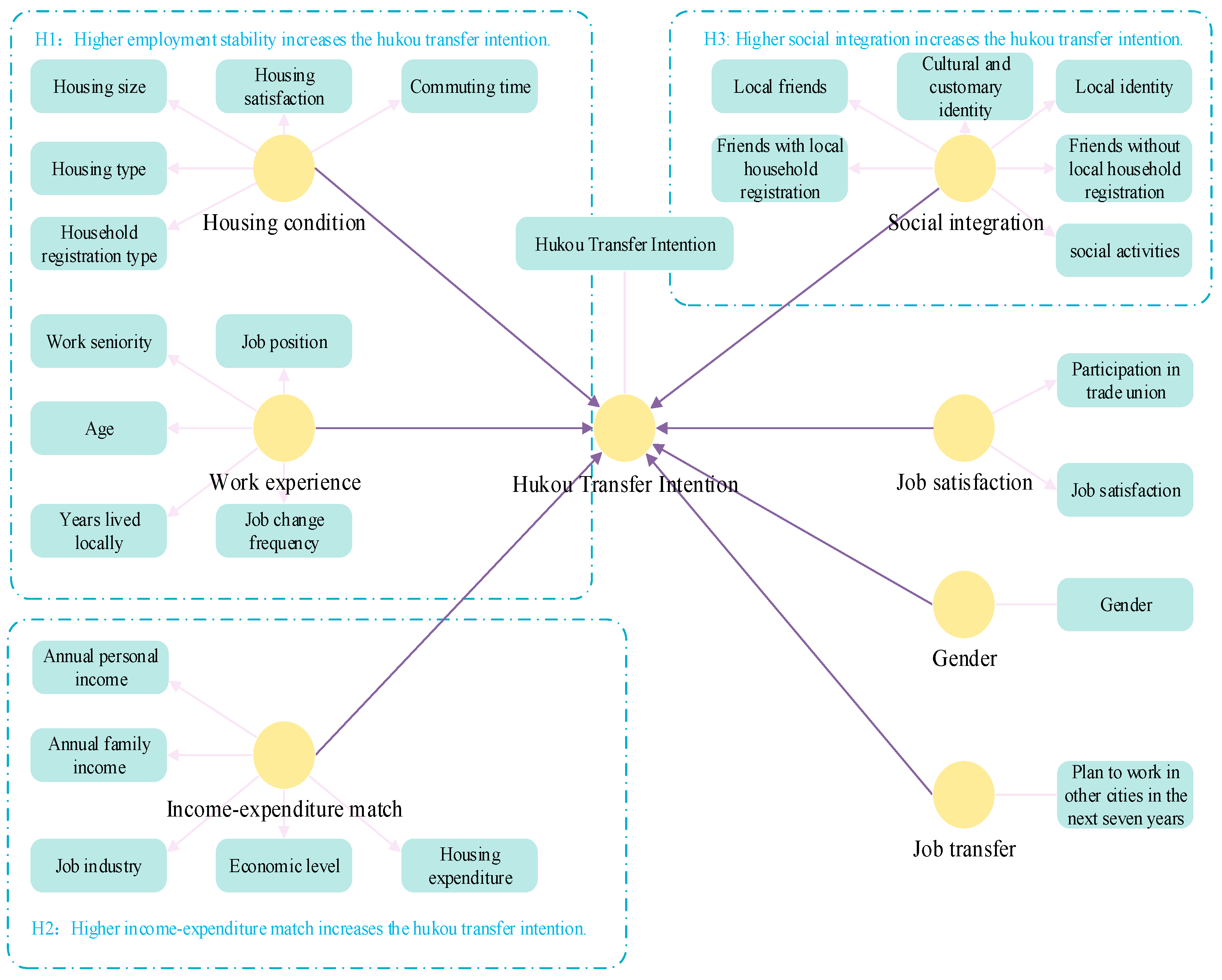
4.3.1. Selection of Latent and Measurement Variables

In this study, the demographic data variables that were significant in the difference analysis, as well as other numerical variables and Likert scale-type items that were significant in the correlation analysis, were selected as explanatory observational variables, with willingness to relocate households as an explanatory observational variable.

For the demographic data variables, the assignment rules in PLS-SEM were as follows: (1) job industry: construction = 1, accommodation and catering and other services = 2, wholesale and retail = 3, manufacturing = 4, transportation and warehousing and postal = 5; (2) gender: male = 1, female = 2; (3) household registration type: rural household registration = 1, urban household registration = 2; (4) plan to work in other cities in the next seven years: impossible = 1, unlikely = 2, normal = 3, likely = 4, probably = 5; (5) job position: grassroots = 1, low = 2, middle = 3, high = 4, top = 5; and (6) housing type: free staff dormitory = 1, public rental housing = 2, company rental housing = 3, rental housing in urban village = 4, self-purchased commercial housing = 5, leased commercial housing = 6, others = 7. The structural equation modeling used in this study included eight latent variable dimensions. The latent variable dimensions and the corresponding manifest variables they contained are shown in the table below.

Table 6. Latent variables and corresponding manifest variables.

Latent Variable	Corresponding Manifest Variables
Migration intention	Do you want to migrate your household registration to local government?
Gender	What is your gender?
Job transfer	Do you have any plans to work in other cities in the next 7 years?
Housing condition	What is your household registration type?
	What is your current housing type?
	What is the size in square meters of your current apartment?
	How many minutes does it take you to get from work to home?
	How satisfied are you with your current home overall?
Work experience	How long have you been local?
	How many years have you been with your present employer?
	What is your age?
	How many times have you changed jobs since you arrived?
	What is your present job position?
Income–expenditure	How much is your personal annual income?
	How much is your family annual income?
	How much is your monthly housing expenditure?
	What is your job industry?
	How do you feel about your local economic level compared to those around you?
Social integration	How often do you participate in local social activities?
	How many local friends do you have?
	How many friends with local household registration do you have?
	How many friends without local household registration do you have?
	Do you consider yourself a member of the local population?
	Do you identify with the local culture?
Job satisfaction	Do you participate in trade union activities?
	Are you satisfied with your present work?

shows the relationship between latent variables and the corresponding manifest variables.

4.3.2. Tests of Reliability and Validity

The reliability and validity tests are primary steps to examine the data quality and goodness-of-fit of the structural equation model. The main indices subjected to reliability examination are Cronbach’s alpha (CA) [100], ${\rho }_A$ [101], and composite reliability (CR) [102]. And the common indicator employed to examine validity is the average variance extracted (AVE) [103]. The formulas of these four indicators are:

$$C{A}_j={\displaystyle \frac{p_j}{p_j-1}}\left[1-{\displaystyle \frac{{\displaystyle {\sum }_{h=1}^{p_j}\mathrm{Var}\left(x_{jh}\right)}}{\mathrm{Var}\left(X\right)}}\right],$$

(12)

$${\rho }_{Aj}={\left({{\widehat{w}}^{\prime }}_j{\widehat{w}}_j\right)}^2{\displaystyle \frac{{{\widehat{w}}^{\prime }}_j\left({\mathrm{S}}_j-\mathrm{diag}\left({\mathrm{S}}_j\right)\right){\widehat{w}}_j}{{{\widehat{w}}^{\prime }}_j\left({\widehat{w}}_j{{\widehat{w}}^{\prime }}_j-\mathrm{diag}\left({\widehat{w}}_j{{\widehat{w}}^{\prime }}_j\right)\right){\widehat{w}}_j}},$$

(13)

$$C{R}_j={\displaystyle \frac{{\left({\displaystyle {\sum }_{h=1}^{p_j}{\lambda }_{jh}}\right)}^2}{{\left({\displaystyle {\sum }_{h=1}^{p_j}{\lambda }_{jh}}\right)}^2+{\displaystyle {\sum }_{h=1}^{p_j}{e}_{jh}^2}}},$$

(14)

$$AV{E}_j={\displaystyle \frac{{\displaystyle {\sum }_{h=1}^{p_j}{\lambda }_{jh}^2}}{{\displaystyle {\sum }_{h=1}^{p_j}{\lambda }_{jh}^2}+{\displaystyle {\sum }_{h=1}^{p_j}{e}_{jh}^2}}},$$

(15)

where $p_j$ is the number of manifest variables corresponding to the $j$-th latent variable;$\mathrm{Var}\left(X\right)$ represents the variance of total sample; ${\lambda }_{jh}$ and $e_{jh}$ are the loading factor and measurement error of the $h$-th manifest variable of the $j$-th latent variable, respectively; ${\widehat{w}}_j$ is the estimated weight vector of the $j$-th latent variable; and ${\mathrm{S}}_j$ represents the empirical covariance matrix of the corresponding manifest variables of the $j$-th latent variable.

Reliability tests were conducted to ensure the internal consistency reliability and composite reliability. Specifically, the internal consistency reliability was evaluated by CA. In general, a CA greater or equal to 0.80 indicates a good scale, 0.70 an acceptable scale, and 0.60 a scale of exploratory purposes [104]. In reaction to CA’s inappropriateness in underestimating the reliability when tau-equivalence was not met or if the sample size was small, [101] proposed a consistent reliability coefficient ${\rho }_A$. In practice, a ${\rho }_A$ larger than 0.7 will suffice. CR was further employed to examine the composite reliability, which represents a significant difference among the average of all sample groups and expresses the uniformity of the manifest variables of each latent variable. The common threshold value for CR is 0.7 [105].

Table 7. Results of reliability and validity tests.

Latent Variables	CA	${\mathit{\rho }}_{\mathit{A}}$	CR	AVE
Housing condition	0.655	0.669	0.786	0.430
Job satisfaction	0.665	0.731	0.852	0.743
Job transfer	1.000	1.000	1.000	1.000
Work experience	0.671	0.723	0.785	0.430
Gender	1.000	1.000	1.000	1.000
Migration intention	1.000	1.000	1.000	1.000
Income–expenditure	0.684	0.716	0.803	0.465
Social integration	0.837	0.856	0.884	0.566

shows that, for each of the latent variables, CA, ${\rho }_A$, and CR were all above 0.6, indicating that the constructs exhibited good reliability.

Validity tests of the PLS-SEM included examinations of both the convergence validity and the discriminant validity. Convergence validity refers to the fact that the manifest variables measuring the same latent variable will fall on a common factor. The convergence validity was primarily examined by AVE. Ref. [102] suggested 0.5 as the critical standard of AVE. An AVE over than 0.5 indicates the latent variable has a high degree of convergence validity. Ref. [106] further argued that if AVE is between 0.4 to 0.5, but the composite reliability is higher than 0.6, the convergent validity of the construct is still adequate. Table 7 shows that the convergence validity of each latent variable met the requirement, reflecting a good linear equivalence relation between the manifest indicators and the corresponding latent variable. Discriminant validity, on the other hand, is an indicator that characterizes the differentiation between latent variables [107]. A structural equation model is considered to have good discriminant validity if the square root of AVE of each latent variable is greater than the respective correlation coefficient with other latent variables.

Table 8. Results of the Fornell–Larker criterion.

Latent Variables	(1)	(2)	(3)	(4)	(5)	(6)	(7)	(8)
Housing condition	0.656
Job satisfaction	0.150	0.862
Job transfer	−0.166	−0.177	1.000
Work experience	0.490	0.088	−0.181	0.655
Gender	0.155	−0.144	−0.057	−0.039	1.000
Migration intention	0.450	0.269	−0.209	0.422	0.143	1.000
Income–expenditure	0.541	0.033	−0.189	0.463	0.117	0.400	0.682
Social integration	0.278	0.576	−0.165	0.353	−0.024	0.487	0.175	0.752

illustrates the discriminant validity examination results by means of the Fornell–Larker criterion. The diagonal is the square root of AVE, while the non-diagonals are the correlation coefficients between two latent variables. According to Table 7, the square root of AVE exceeds the correlation coefficients, except for the self-constructed second-order latent variable knowledge. The results verify a satisfying discriminant validity.

Another commonly used discriminant validity examination is the heterotrait–monotrait ratio (HTMT). This is the ratio of the means of the correlation coefficients of indicators between different latent variables to the means of the correlation coefficients of indicators within the same latent variable. The conservative threshold for HTMT is 0.85. The threshold for HTMT can be relaxed to 0.90 when the latent variables are conceptually similar.

Table 9. Results of the HTMT.

Latent Variables	(1)	(2)	(3)	(4)	(5)	(6)	(7)	(8)
Housing condition
Job satisfaction	0.322
Job transfer	0.208	0.235
Work experience	0.693	0.255	0.223
Gender	0.231	0.180	0.057	0.149
Migration intention	0.554	0.321	0.209	0.458	0.143
Income–expenditure	0.804	0.272	0.229	0.598	0.193	0.479
Social integration	0.457	0.780	0.176	0.446	0.055	0.526	0.277

demonstrates the results of HTMT, which can be seen to all be less than the conservative threshold of 0.85, demonstrating good discriminant validity. In summary, the goodness of the reliability and validity tests indicates the soundness of the calculation results gained from the constitutive structural equation model.

4.3.3. Path Analysis

By conducting the PLS algorithm, the path coefficients between latent variables could be derived, and they are displayed in Figure 2. The values of the path coefficients reflect, to some extent, the strength of the interaction between latent variables. However, further statistical tests are needed for the significance tests of the path coefficients. Since PLS does not make assumptions about the normality distribution of the data, the parametric significance tests (e.g., t-test or z-test) cannot be applied to examine the significance of PLS-SEM’s path coefficients. Instead of parametric significance tests, a nonparametric bootstrap procedure can be utilized. The bootstrap method constructs subsets of the existing sample data by means of constant random sampling. The distribution of original samples can be adequately denoted through repeatedly creating subsamples [108]. For each subsample, the PLS algorithm is applied to obtain estimation of path coefficients. After traversing each subset, the mean and standard deviation of each path coefficient can be obtained. Then, t-tests can be further performed to evaluate the significance of each path coefficient. This study adopts the bias-corrected and accelerated bootstrap methods [109]. The number of subsamples was set to 5000, and a one-tailed t-test was conducted.

The overall goodness of fit (R Square) of the model reached 0.400, and the adjusted R Square-adjusted reached 0.377, indicating that the seven explanatory latent variable dimensions can explain 37.7% of the total variance information of the willingness to relocate households, and that the explanatory effect is good. At the significance level of 0.05, the results of the path analysis show that: (1) Housing condition plays a significant positive explanatory role in migration intention (t = 2.277, p = 0.011); (2) work experience plays a significant, positive explanatory role in migration intention (t = 2.004, p = 0.023); (3) gender plays a significant, positive explanatory role in migration intention (t = 1.904, p = 0.028); (4) income–expenditure has a significant positive explanatory effect on migration intention (t = 1.950, p = 0.026); (5) social integration has a significant positive explanatory effect on migration intention (t = 4.824, p = 0.000); and (6) job satisfaction and job transfer may have no statistically significant influence on the non-statistically significant effect on migration intention.

Table 10. Significance test of path coefficients.

Path	Coefficient	Standard Deviation	t Statistic	p-Value
Housing condition → Intention	0.170	0.074	2.277	0.011
Job satisfaction → Intention	0.047	0.065	0.638	0.262
Job transfer → Intention	−0.054	0.059	0.967	0.167
Work experience → Intention	0.139	0.069	2.004	0.023
Gender → Intention	0.111	0.060	1.904	0.028
Income–expenditure → Intention	0.171	0.083	1.950	0.026
Social integration → Intention	0.332	0.069	4.824	0.000

shows the results.

5. Conclusions

This study examines the influence of employment quality on the hukou transfer intentions of the new generation of migrant workers. Specifically, latent variables such as migration intentions, housing situations, work experience, income–expenditure, social integration, and job satisfaction were measured using corresponding manifest variables. The study conducted differential and correlation analyses and empirical PLS-SEM analysis, completing a path analysis of how employment quality impacts migration intentions.

The findings reveal that multiple factors affect the migration intentions of migrant workers, with employment quality having a strong positive influence. First, differential analysis based on demographic characteristics showed that job industry, gender, type of household registration, job positions, housing types, and parental living conditions are significantly correlated with migration intentions at the 0.05 level; at the 0.10 level, whether parents are local and whether one plans to work in other cities in the next seven years also significantly affect migration intentions. Second, correlation analysis of numerical variables showed that age, local family members, years lived locally, job change frequency, work seniority, and job satisfaction are positively correlated with migration intentions, with income, local friends, and housing size having the highest correlation coefficients, while weekly working hours and number of housing residents showed significant negative correlations with migration intentions. Third, empirical analysis using the PLS-SEM model confirmed all hypotheses: Higher employment stability (including housing condition (p = 0.011) and work experience (p = 0.023), better income–expenditure match (p = 0.026), and greater social integration (p = 0.000) all positively affect migration intentions).

As the primary component of the floating population, migrant workers are not only the backbone of China’s economic growth, but also pivotal in advancing urbanization and enhancing its quality. Accelerating the migration of migrant workers is instrumental in promoting social equity in China, balancing regional economic development, and fostering a harmonious and civilized society. The results have practical implications for government agencies formulating targeted policies to enhance the migration intentions of migrant workers.

The suggestions for improving employment stability include improving labor remuneration, safeguarding labor rights, stabilizing labor demand, and eliminating labor discrimination to improve the employment quality of the new generation of migrant workers, fostering a sense of urban belonging and identity, accelerating migration, and promoting social equity and balanced regional economic development. In terms of enhancing labor remuneration, the government can collaborate with businesses to actively conduct vocational training, improving migrant workers’ skills and overall qualifications and helping them to secure higher wages in the labor market. In safeguarding labor rights, expanding legal education coverage to raise awareness among migrant workers, improving current legal aid mechanisms for timely relief, and strengthening corporate oversight to prevent rights infringements are critical. In stabilizing labor market demand, improving current job platforms to reduce the costs of job transitions for migrant workers is essential, as well as establishing housing security mechanisms and encouraging qualified businesses to provide temporary residences or transportation to reduce the costs associated with changes in residence and commuting for migrant workers. To eliminate labor discrimination, building community platforms to foster cultural integration and actively promoting professional equality to prevent discriminatory practices ensure that migrant workers are treated with respect and equality.

China’s vastness makes conducting a large-scale comprehensive survey costly. As a cutting-edge exploratory study, this research offers preliminary insights into the factors influencing migrant workers’ willingness to relocate their household registration based on a sample of 195 migrant workers. In future research, we plan to conduct a larger-scale survey to significantly increase the sample size. Additionally, since the majority of the migrant workers in our current sample are employed in the construction industry, future research will aim to diversify the data by including respondents from different industries.

References

1. He, C.; Jin, W. A Study on Migrant Workers’ Permanent Migration Intentions. Sociol. Stud. 2007, 6, 86–113, 243. [Google Scholar]
2. Wei, Y.; Wang, Z.; Wang, H.; Li, Y.; Jiang, Z. Predicting population age structures of China, India, and Vietnam by 2030 based on compositional data. PLoS ONE 2019, 14, e0212772. [Google Scholar] [CrossRef]
3. Hatton, T.J.; Williamson, J.G. Demographic and Economic Pressure on Emigration out of Africa. Scand. J. Econ. 2003, 105, 465–486. [Google Scholar] [CrossRef]
4. Mayda, M.A. International migration: A panel data analysis of the determinants of bilateral flows. J. Popul. Econ. 2010, 23, 1249–1274. [Google Scholar] [CrossRef]
5. Adsera, A.; Chiswick, R.B. Are there gender and country of origin differences in immigrant labor market outcomes across European destinations? J. Popul. Econ. 2007, 20, 495–526. [Google Scholar] [CrossRef]
6. Sheng, Y. Gradient effect and influence mechanism of migrant’s residence preference. China Popul. Resour. Environ. 2017, 27, 128–136. [Google Scholar]
7. Chen, G.; Wei, X.; Wang, G. Study on the Influencing Factors of Rural-Urban Migrant Workers’ Willingness to be Urban Citizens in Shanghai. Popul. Dev. 2010, 16, 2–11. [Google Scholar]
8. Wang, G.; Wu, J. Influence Factors Analysis of Social Distance between Migrants and Residents in Shanghai. Sociol. Stud. 2011, 25, 28–47, 243. [Google Scholar]
9. Zhou, C. The Impact of Job Stability on Migrant Workers’ Permanent Migration Intention. Popul. Dev. 2022, 28, 148–160. [Google Scholar]
10. Yao, J. Willingness survey on the desire to settle in cities of rural laborers: An empirical analysis in three cities of Jiangsu. Urban Probl. 2009, 96–101. [Google Scholar]
11. Zhang, P.; Hao, Y.B.; Chen, W.M. Happiness, Social Integration and Migration Decision. Econ. Rev. 2014, 1, 58–69. [Google Scholar]
12. Meng, Y.; Deng, D. The “Income Paradox” in the Course of Migrant Workers Integrating into Cities: The Case of Wuhan City. Chin. J. Popul. Sci. 2011, 74–82, 112. [Google Scholar]
13. Liu, C.; Zhou, L. Urban integration of social capital and migrant workers. Popul. Res. 2004, 5, 12–18. [Google Scholar]
14. Zhang, Y. Migrant Workers’ Willing of Hukou Register and Policy Choice of China Urbanization. Chin. J. Popul. Sci. 2011, 14–26, 111. [Google Scholar] [CrossRef]
15. Dong, X. Housing Affordability and Permanent Migration Desire of Rural-Urban Migrants. Chin. J. Popul. Sci. 2015, 91–99, 128. [Google Scholar]
16. Han, Q.; Chen, X. The Impact of Labour Relations on Intentions of Household Registrations in Small and Medium-sized Towns for Migrant Workers: A Study Based on an Investigation of 151 Enterprises in Guangdong Province. Chin. J. Popul. Sci. 2016, 101–109, 128. [Google Scholar]
17. Lin, L.; Zhu, Y. Spatial variation and its determinants of migrants’ Hukou transfer intention of China’s prefecture- and provincial-level cities: Evidence from the 2012 national migrant population dynamic monitoring survey. Acta Geogr. Sin. 2016, 71, 1696–1709. [Google Scholar]
18. Feng, H. Research on the Factors that Effect the Employment Training Needs of Migrant Workers in Sichuan; Sichuan University: Chengdu, China, 2011. [Google Scholar]
19. Lam, L.W. Impact of competitiveness on salespeople’s commitment and performance. J. Bus. Res. 2012, 65, 1328–1334. [Google Scholar] [CrossRef]
20. Yang, J.H.; Zhang, J.J.; Wu, M. My Home Is Where My Heart Is: Regional Disparity and Self-identity of Migrants in China. Popul. Econ. 2016, 4, 21–33. [Google Scholar]
21. Li, Z.; Yuan, L. The Effects of Working Distance on Employment Quality of Rural Migrant Workers. Chin. Rural. Econ. 2017, 6, 70–83. [Google Scholar]
22. Dolfin, S.; Genicot, G. What Do Networks Do? The Role of Networks on Migration and “Coyote” Use. Rev. Dev. Econ. 2010, 14, 343–359. [Google Scholar] [CrossRef]
23. Duan, C.; Lv, L.; Zou, X. Major Challenges for China’s Floating Population and Policy Suggestions: An Analysis of the 2010 Population Census Data. Popul. Res. 2013, 37, 17–24. [Google Scholar]
24. Ming, J.; Zeng, X. Job switching and employment quality of migrant workers: Influence effect and transmission mechanism. Econ. Perspect. 2015, 12, 22–33. [Google Scholar]
25. Zhang, Q. A theoretical discussion on the stability and fluctuation of peasant employment. J. Univ. Chin. Acad. Soc. Sci. 1993, 1, 45–51. [Google Scholar]
26. Xie, Y. Job Stability and Urban Integration of New Generation Migrant Workers: Example of Casein Jiangsu Province. Issues Agric. Econ. 2015, 36, 54–62, 111. [Google Scholar]
27. Maxwell, R. Evaluating Migrant Integration: Political Attitudes Across Generations in Europe. Int. Migr. Rev. 2010, 44, 25–52. [Google Scholar] [CrossRef]
28. Shi, Z.; Liu, S.; Zhao, Y. The Paradox of Unstable Employment and the Citizenization of Migrant Workers: Based on the Perspective of Labor Process. Chin. J. Sociol. 2022, 42, 88–123. [Google Scholar]
29. Lu, W.; Zhang, B. Employment Type, Social Welfare and Urban Integration of Floating Population—Evidence from Microdata. Economist 2018, 8, 34–41. [Google Scholar]
30. Wang, Y. Settlement Intention of Rural Migrants in Chinese Cities: Findings from a Twelve-city Migrant Survey. Popul. Res. 2013, 37, 19–32. [Google Scholar]
31. Su, Q.; Zhao, X.; Ji, L. The Migrant Workers’ Mental Health Study Based on Deprivation Theory. J. Huazhong Agric. Univ. Soc. Sci. Ed. 2016, 93–101, 145–146. [Google Scholar]
32. Hong, J.; Ni, C. The Quality of Urban Public Service Supply and Migrant Workers’ Settlement Choice. Chin. J. Popul. Sci. 2020, 54–65, 127. [Google Scholar]
33. Brown, R.N. Housing Experiences of Recent Immigrants to Canada’s Small Cities: The Case of North Bay, Ontario. J. Int. Migr. Integr. 2017, 18, 719–747. [Google Scholar] [CrossRef]
34. Qiu, A.; Wang, J.; Ding, C. Migrant Housing during Rapid Urbanization in China: Typology and Assessment. Urban Stud. 2011, 18, 49–54. [Google Scholar]
35. Rockwood, D.; Tran, Q.D. Urban immigrant worker housing research and design for Da Nang, Viet Nam. Sustain. Cities Soc. 2016, 26, 108–118. [Google Scholar] [CrossRef]
36. Dimitris, B. Housing Pathways of Immigrants in the City of Athens: From Homelessness to Homeownership. Considering Contextual Factors and Human Agency. Hous. Theory Soc. 2020, 37, 230–250. [Google Scholar]
37. Alvarez, L.A.; Müller-Eie, D. Housing circumstances and quality of life among local and immigrant population in Norwegian neighbourhoods. J. Hous. Built Environ. 2021, 37, 1–22. [Google Scholar]
38. Simone, D.; Newbold, B.K. Housing Trajectories Across the Urban Hierarchy: Analysis of the Longitudinal Survey of Immigrants to Canada, 2001–2005. Hous. Stud. 2014, 29, 1096–1116. [Google Scholar] [CrossRef]
39. Zhu, P.; Zhao, S.; Jiang, Y. Residential segregation, built environment and commuting outcomes: Experience from contemporary China. Transp. Policy 2022, 269–277. [Google Scholar] [CrossRef]
40. Feng, C.; Liu, B. Commuting Pattern and Spatial Relation between Residence and Employment of Migrant Workers in Metropolitan Areas: The Case of Beijing. Urban Plan. Forum 2012, 4, 59–64. [Google Scholar]
41. Zeng, Y.; Zhang, L. Discrimination against Rural Migrant Workers and Their Wage Diminish: New Evidence from the 2015 National Floating Population’s Dynamic Monitoring Survey. J. Zhongnan Univ. Econ. Law 2018, 5, 141–150. [Google Scholar]
42. Li, Q.; Hu, B. Reform of Household Registration System and the Path of Migrant Workers Citizenization. Sociol. Rev. China 2013, 1, 36–43. [Google Scholar]
43. Farber, H.S. The Analysis of Interfirm Worker Mobility. J. Labor Econimics 1994, 12, 554–593. [Google Scholar] [CrossRef]
44. Deng, R. How Does the Relationship Resource in Social Capital Mobilization Affect the Employment Quality of Migrant Workers? Econ. Perspect. 2020, 1, 52–68. [Google Scholar]
45. Liu, Z. Institution and inequality: The hukou system in China. J. Comp. Econ. 2004, 33, 133–157. [Google Scholar] [CrossRef]
46. Zhao, Y. Causes and Consequences of Return Migration: Recent Evidence from China. J. Comp. Econ. 2002, 30, 376–394. [Google Scholar] [CrossRef]
47. Yakushko, O. Career Development Concerns of Recent Immigrants and Refugees. J. Career Dev. 2008, 34, 362–396. [Google Scholar] [CrossRef]
48. Abramsson, M.; Fransson, L.E.B.U. Housing Careers: Immigrants in Local Swedish Housing Markets. Hous. Stud. 2002, 17, 445–464. [Google Scholar] [CrossRef]
49. Meng, X. The Informal Sector and Rural-Urban Migration—A Chinese Case Study. Asian Econ. J. 2001, 15, 71–89. [Google Scholar] [CrossRef]
50. Akhlaq, A. Does additional work experience moderate ethnic discrimination in the labour market? Econ. Ind. Democr. 2022, 43, 1119–1142. [Google Scholar]
51. Schultz. Investment in Human Capital. Am. Econ. Rev. 1961, 51, 1–17. [Google Scholar]
52. Zhu, Y.; Chen, W. The settlement intention of China’s floating population in the cities: Recent changes and multifaceted individual-level determinants. Popul. Space Place 2010, 16, 253–267. [Google Scholar] [CrossRef]
53. Lewis, W.A. Economic Development with Unlimited Supplies of Labour. Manch. Sch. 1954, 22, 139–191. [Google Scholar] [CrossRef]
54. Chen, W. Economic incentives and settlement intentions of rural migrants: Evidence from China. J. Urban Aff. 2019, 41, 372–389. [Google Scholar] [CrossRef]
55. Gu, H. Understanding the migration of highly and less-educated labourers in post-reform China. Appl. Geogr. 2021, 137. [Google Scholar] [CrossRef]
56. Zhou, C.; Wu, F.; Zhang, J. Balance change and cross-regional return trend of rural migrant labor in China. J. Agrotech. Econ. 2016, 4, 4–15. [Google Scholar]
57. Calvo, R.; Cheung, F. Does Money Buy Immigrant Happiness? J. Happiness Stud. 2018, 19, 1657–1672. [Google Scholar] [CrossRef]
58. Basavarajappa, K.G.; Halli, S.S. A Comparative Study of Immigrant and Non-immigrant Families in Canada with Special Reference to Income, 1986. Int. Migr. Migr. Int. Migr. Int. 2010, 35, 225–252. [Google Scholar] [CrossRef]
59. Tong, Y.; Wang, Y. The Choice of Floating Migrants in China: Why Megacities are Always Preferred? A Cost-Benefit Analysis. Popul. Res. 2015, 39, 49–56. [Google Scholar]
60. Guo, F.; Iredale, R. The Impact of Hukou Status on Migrants’ Employment: Findings from the 1997 Beijing Migrant Censusl. Int. Migr. Rev. 2004, 38, 709–731. [Google Scholar] [CrossRef]
61. Zhang, Y.; Cen, Q. Spatial Patterns of Population Mobility and Determinants of Inter-provincial Migration in China. Popul. Res. 2014, 38, 54–71. [Google Scholar]
62. Gokdemir, O.; Dumludag, D. Life Satisfaction Among Turkish and Moroccan Immigrants in the Netherlands: The Role of Absolute and Relative Income. Soc. Indic. Res. 2012, 106, 407–417. [Google Scholar] [CrossRef]
63. McConnell, D.E.; Akresh, R.I. Housing Cost Burden and New Lawful Immigrants in the United States. Popul. Res. Policy Rev. 2010, 29, 143–171. [Google Scholar] [CrossRef]
64. Maria, C.L.; Varisa, R.P.; Suzie, W. The Impact of Housing Experience on the Well-Being of 1.5-Generation Immigrants: The Case of Millennial and Gen-Z Renters in Southern California. Hous. Policy Debate 2023, 33, 224–250. [Google Scholar]
65. Wu, X.; Yuan, M. Analysis on social and cultural influencing factors of migrant workers’ migration decision. Chinese Rural Economy 2005, 26–32, 39. [Google Scholar]
66. Liu, J.; Wei, H. How Does Dialect Distance Affect Permanent Migration Intension of Migrant Workers: From the Perspective of Social Integration. China Rural. Surv. 2022, 1, 34–52. [Google Scholar]
67. Harder, N.; Figueroa, L.; Gillum, R.M.; Hangartner, D.; Laitin, D.D.; Hainmueller, J. Multidimensional measure of immigrant integration. Proc. Natl. Acad. Sci. USA 2018, 115, 11483–11488. [Google Scholar] [CrossRef]
68. Huang, X.; Liu, Y.; Xue, D.; Li, Z.; Shi, Z. The effects of social ties on rural-urban migrants’ intention to settle in cities in China. Cities 2018, 83, 203–212. [Google Scholar] [CrossRef]
69. Liu, Y.; Pan, Z.; Liu, Y.; Chen, H.; Li, Z. Where Your Heart Belong to shapes how you feel about yourself: Migration, social comparison and subjective well-being in China. Popul. Space Place 2020, 26, e2336. [Google Scholar] [CrossRef]
70. Chen, S.; Liu, Z. What determines the settlement intention of rural migrants in China? Economic incentives versus sociocultural conditions. Habitat Int. 2016, 58, 42–50. [Google Scholar] [CrossRef]
71. Leszczensky, L.; Stark, T.H.; Flache, A.; Munniksma, A. Disentangling the relation between young immigrants’ host country identification and their friendships with natives. Soc. Netw. 2016, 44, 179–189. [Google Scholar] [CrossRef]
72. Li, C. An Analysis of Factors Affecting Rural Migrant Workers’ Collective Action—Based on a Survey of Migrant Workers in the Pearl River Delta Region. China Rural. Surv. 2009, 6, 96. [Google Scholar]
73. Ye, P. Residential Preferences of Migrant Workers: An Analysis of the Empirical Survey Data from Seven Provinces/Districts. Chin. J. Sociol. 2011, 31, 153–169. [Google Scholar]
74. Li, P.; Tian, F. A Cross Generational Comparison of the Social Cohesion of Migrant Workers in China. Chin. J. Sociol. 2012, 32, 1–24. [Google Scholar]
75. Chu, R.; Xiong, Y.; Yi, Z. The Determinant Factors of Migrant Workers’ Social Identity: An Empirical Study in Shanghai. Chin. J. Sociol. 2014, 34, 25–48. [Google Scholar]
76. ChulHo, B.; JoonHee, L.; Chulhwan, C. The Effects of Leisure Activities on Self-Efficacy and Social Adjustment: A Study of Immigrants in South Korea. Int. J. Environ. Res. Public Health 2021, 18, 8311. [Google Scholar] [CrossRef]
77. Alfieri, S.; Marzana, D.; D’Angelo, C.; Corvino, C.; Gozzoli, C.; Marta, E. Engagement of young immigrants: The impact of prosocial and recreational activities. J. Prev. Interv. Community 2021, 50, 11–17. [Google Scholar] [CrossRef]
78. Schwartz, S.J.; Montgomery, M.J.; Briones, E. The Role of Identity in Acculturation among Immigrant People: Theoretical Propositions, Empirical Questions, and Applied Recommendations. Hum. Dev. 2006, 49, 1–30. [Google Scholar] [CrossRef]
79. Weber, S.; Kronberger, N.; Appel, M. Immigrant students’ educational trajectories: The influence of cultural identity and stereotype threat. Self Identity 2018, 17, 211–235. [Google Scholar] [CrossRef]
80. Carpentier, J.; Sablonnière, L.E.R. Identity profiles and well-being of multicultural immigrants: The case of Canadian immigrants living in Quebec. Front. Psychol. 2013, 4, 80. [Google Scholar] [CrossRef]
81. Baruch, Y.; Holtom, B.C. Survey response rate levels and trends in organizational research. Hum. Relat. 2008, 61, 1139–1160. [Google Scholar] [CrossRef]
82. Wold, H. Path models with latent variables: The NIPALS approach. In Quantitative Sociology; Academic Press: Cambridge, MA, USA, 1975; pp. 307–357. [Google Scholar]
83. Wold, H. Soft modeling: The basic design and some extensions. Syst. Under Indirect. Obs. 1982, 2, 343. [Google Scholar]
84. Hair, J.F.; Risher, J.J.; Sarstedt, M.; Ringle, C.M. When to use and how to report the results of PLS-SEM. Eur. Bus. Rev. 2019, 31, 2–24. [Google Scholar] [CrossRef]
85. Li, Y.; Wang, Z.; Wei, Y. Pathways to progress sustainability: An accurate ecological footprint analysis and prediction for Shandong in China based on integration of STIRPAT model, PLS, and BPNN. Environ. Sci. Pollut. Res. 2021, 28, 54695–54718. [Google Scholar] [CrossRef]
86. Sarstedt, M.; Ringle, C.M.; Hair, J.F. Partial least squares structural equation modeling. Handb. Mark. Res. 2017, 26, 1–40. [Google Scholar]
87. Li, Y.; Wei, Y.G.; Dong, Z.; Huo, Y. Impacts of Demographic Factors on Carbon Emissions Based on the STIRPAT Model and the PLS Method: A Case Study of Shanghai. Environ. Eng. Manag. J. 2020, 19, 1443–1458. [Google Scholar]
88. Hair, J.F.; Sarstedt, M.; Pieper, T.M.; Ringle, C.M. The use of partial least squares structural equation modeling in strategic management research: A review of past practices and recommendations for future applications. Long Range Plan. 2012, 45, 320–340. [Google Scholar] [CrossRef]
89. Nitzl, C. The use of partial least squares structural equation modelling (PLS-SEM) in management accounting research: Directions for future theory development. J. Account. Lit. 2016, 37, 19–35. [Google Scholar] [CrossRef]
90. Willaby, H.W.; Costa, D.S.; Burns, B.D.; MacCann, C.; Roberts, R.D. Testing complex models with small sample sizes: A historical overview and empirical demonstration of what partial least squares (PLS) can offer differential psychology. Personal. Individ. Differ. 2015, 84, 73–78. [Google Scholar] [CrossRef]
91. Hair, J.; Hollingsworth, C.L.; Randolph, A.B.; Chong AY, L. An updated and expanded assessment of PLS-SEM in information systems research. Ind. Manag. Data Syst. 2017, 117, 442–458. [Google Scholar] [CrossRef]
92. Reinartz, W.; Haenlein, M.; Henseler, J. An empirical comparison of the efficacy of covariance-based and variance-based SEM. Int. J. Res. Mark. 2009, 26, 332–344. [Google Scholar] [CrossRef]
93. Mooi, E.; Sarstedt, M. A Concise Guide to Market Research the Process, Data, and Methods Using IBM SPSS Statistics; Springer: Berlin/Heidelberg, Germany, 2011. [Google Scholar]
94. Boadi, E.B.; Wenxin, W.; Bentum-Micah, G.; Asare IK, J.; Bosompem, L.S. Impact of service quality on customer satisfaction in Ghana hospitals: A PLS-SEM approach. Can. J. Appl. Sci. Technol. 2019, 7, 503–511. [Google Scholar]
95. Al-Emran, M.; Mezhuyev, V.; Kamaludin, A. PLS-SEM in information systems research: A comprehensive methodological reference. In Proceedings of the International Conference on Advanced Intelligent Systems and Informatics, Cairo, Egypt, 1–3 September 2018; Springer: Cham, Switzerland, 2018; pp. 644–653. [Google Scholar]
96. Pant, M.; Virdi, A.S.; Chaubey, D.S. Examining the effect of marketing innovations on GPMA: A study using the PLS–SEM Approach. Glob. Bus. Rev. 2020, 21, 1025–1036. [Google Scholar] [CrossRef]
97. Sheko, A.; Braimllari, A. Information technology inhibitors and information quality in supply chain management: A PLS-SEM analysis. Acad. J. Interdiscip. Stud. 2018, 7, 125. [Google Scholar] [CrossRef]
98. Hair, J.F.; Sarstedt, M.; Ringle, C.M.; Mena, J.A. An assessment of the use of partial least squares structural equation modeling (PLS-SEM) in hospitality research. Int. J. Contemp. Hosp. Manag. 2018. [Google Scholar]
99. Rehman Khan, S.A.; Yu, Z. Assessing the eco-environmental performance: An PLS-SEM approach with practice-based view. Int. J. Logist. Res. Appl. 2021, 24, 303–321. [Google Scholar] [CrossRef]
100. Cronbach, L.J. Coefficient alpha and the internal structure of tests. Psychometrika 1951, 16, 297–334. [Google Scholar] [CrossRef]
101. Dijkstra, T.K.; Henseler, J. Consistent partial least squares path modeling. MIS Q. 2015, 39, 297–316. [Google Scholar] [CrossRef]
102. Höck, M.; Ringle, C.M. Strategic networks in the software industry: An empirical analysis of the value continuum. In Proceedings of the IFSAM VIIIth World Congress, Berlin, Germany, 28–30 September 2006; Volume 28. [Google Scholar]
103. Bacon, D.R.; Sauer, P.L.; Young, M. Composite reliability in structural equations modeling. Educ. Psychol. Meas. 1995, 55, 394–406. [Google Scholar] [CrossRef]
104. Geladi, P.; Kowalski, B.R. Partial least-squares regression: A tutorial. Anal. Chim. Acta 1986, 185, 1–17. [Google Scholar] [CrossRef]
105. Yao, T.; Wei, Y.; Zhang, J.; Wang, Y.; Yu, Y.; Huang, W. What influences the urban sewage discharge in China? The effect of diversified factors on the urban sewage discharge in different regions of China. Environ. Dev. Sustain. 2021, 24, 6099–6135. [Google Scholar] [CrossRef]
106. Fornell, C.; Larcker, D.F. Evaluating structural equation models with unobservable variables and measurement error. J. Mark. Res. 1981, 18, 39–50. [Google Scholar] [CrossRef]
107. Brayfield, A.H.; Crockett, W.H. Convergent and discriminant validity by the multi-trait, multimethod matrix. Psychol. Bull. 1955, 52, 396–424. [Google Scholar] [CrossRef] [PubMed]
108. Hair, J.F., Jr.; Hult, G.T.M.; Ringle, C.; Sarstedt, M. A Primer on Partial Least Squares Structural Equation Modeling (PLS-SEM); Sage Publications: Thousand Oaks, CA, USA, 2021. [Google Scholar]
109. Diciccio, T.J.; Romano, J.P. A review of bootstrap confidence intervals. J. R. Stat. Soc. Ser. B Methodol. 1988, 50, 338–354. [Google Scholar] [CrossRef]
Figure 1. The influence mechanism of employment quality on hukou transfer intention.
Sustainability 16 07857 g001
Figure 2. The estimated constitutive SEM.
Sustainability 16 07857 g002