Abstract
The macroscopic fundamental diagram (MFD), as a model depicting the correlation between traffic flow parameters at the network level, offers a new way to understand regional traffic state using derived traffic flow data from detectors directly. The accuracy of MFD construction is directly related to factors such as the type of detectors, their distribution, and their quantity within the road network. Understanding these influencing factors and mechanisms is crucial for enhancing the reliability of MFD-based applications such as congestion pricing and threshold control. Present investigations on factors that affect MFD construction’s accuracy have frequently been confined to sensitivity analysis of single-source data and individual influencing factors such as the penetration rate. However, the accuracy of MFD is influenced by a multitude of factors, including the spatial distribution equilibrium, penetration rate, and coverage rate of traffic flow detection equipment. Despite this, this paper utilized the Q-paramics simulation software V6.8.1 to acquire simulated data and employed the orthogonal experimental method from statistics to explore the impact mechanisms of factors on the accuracy of MFD construction. The results of the case study demonstrated that when the penetration rate reaches 20%, the error remains approximately around 10%; once the coverage rate surpasses 45%, the errors stabilize at around 10%. This study provides practical guidance for traffic management and planning decisions aimed at promoting sustainable development through the application of MFD in real-world road networks.
1. Introduction
Accurately understanding the traffic state of urban road networks while optimizing the spatiotemporal distribution of traffic demand to align with road supply capacity is indispensable for alleviating regional traffic congestion. The macroscopic fundamental diagram (MFD) is a model depicting the correlation between network traffic flow, network traffic density, and network traffic speed, etc. It offers a novel avenue to understand the state of regional traffic using derived traffic flow data from detectors directly. Its application spans various domains, including gating control and congestion pricing, etc. Current studies utilizing MFD to determine the traffic state of road networks have certain limitations such as insufficient consideration of the impact of data’s representativeness and comprehensiveness on derived MFD’s accuracy of specific road networks. In other words, the MFD obtained from the complete dataset is accurate (for instance, the MFD derived from all trajectory data within the study area is precise). However, in practical scenarios, we only have access to a subset of the data and the accuracy of the MFD derived from this partial data is influenced by various factors. The methodology for constructing more accurate MFD utilizing multisource data has been proposed and described in our prior research [1]. Building upon this foundation, this paper conducts an analysis of the factors influencing the precision of MFD construction.
The examination of influential factors affecting MFD construction accuracy serves as crucial groundwork for precisely ascertaining the traffic state in road networks. As we know, it is impossible to obtain all traffic flow data with limited detectors for a large-scale road network. The precision of MFD construction is determined by the sample data’s representativeness and comprehensiveness. For multisource data, the factors influencing the accuracy of MFD construction can be summarized as the spatial distribution equilibrium and penetration rate of sample data along with the spatial coverage rate of traffic detection equipment, etc. Present investigations on MFD construction have frequently been confined to a sensitivity analysis of single-source data and individual influencing factors such as penetration rate. However, there exists a necessity for more extensive research encompassing comprehensive analysis, considering the combined impact of spatial distribution equilibrium, penetration rate, and coverage rate, to effectively guide MFD construction using multisource data.
Conducting a comprehensive analysis of the influential factors affecting MFD construction accuracy is difficult with real-world data because of the challenges in obtaining the entire data from real-world road networks and the difficulty in assessing the accuracy of constructed MFD. Traffic simulation software V6.8.1 provides a viable solution. Through simulating traffic flow on real road networks, these software tools can identify traffic zones, calibrate simulation parameters, estimate traffic zones’ origin-destination (OD) demands, and conduct comprehensive traffic simulations, generating a full sample of travel trajectories for all vehicles. By fine-tuning parameters like the positions and coverage rates of simulated detectors and the proportion of simulated floating cars along with their spatial distribution equilibrium on the simulated road network, it becomes feasible to generate simulated multisource sample data. This approach empowers researchers to overcome the limitations of collecting complete sample data from the real world and to explore diverse scenarios to examine the impact of various factors on the accuracy of MFD construction.
Conducting a comprehensive analysis of the influential factors affecting MFD construction accuracy using simulated data involves many influencing factors and their respective levels. Undertaking a full-factor simulation experiment by systematically combining all factors and levels would require substantial effort. For instance, for a six-factor, three-level experiment, a comprehensive test would require 36 = 729 individual trials. Adding even a single additional factor would triple the number of required experiments. Hence, the crucial matter lies in devising a rational experimental plan to simulate diverse complex scenarios and evaluate the data’s adaptability. Such knowledge serves as a fundamental guiding principle for precisely constructing MFDs in real-world road networks.
In light of these considerations, this paper utilizes the Q-paramics simulation software V6.8.1 to acquire simulated data and employs the orthogonal experimental method from statistics to explore the impact mechanisms of factors on the accuracy of MFD construction using multisource data. By quantifying the errors of constructed MFD across diverse data scenarios to explore the data adaptability in various contexts, the results of the case study demonstrated the following:
- (1)
- when the penetration rate reaches 20%, the error remains approximately around 10%;
- (2)
- once the coverage rate surpasses 45%, the errors stabilize at around 10%;
- (3)
- when the fixed detector coverage exceeds 45%, the penetration rate of floating cars is above 10% and the spatial distribution of floating cars is either “moderate” or “strong”, the median error in MFD construction is around 8~10%;
- (4)
- when the fixed detector coverage is below 30%, the penetration rate of floating cars is less than 15% and the spatial distribution of floating cars is mostly “weak”, the median error in MFD construction is around 10~20%.
This study offers practical guidance for constructing MFDs that promote sustainable development in real-world road networks. Specifically, it can assist policymakers in optimizing traffic management strategies, such as threshold control and congestion charging, by improving traffic distribution across the network, enhancing efficiency, and reducing both carbon emissions and the waste of road resources.
2. Literature Review
With the continuous deepening of theoretical research on MFD, it has sparked widespread discussions on the influencing factors of MFD. Recent studies have indicated that the primary determinants affecting MFD are the conditions of roadways, control measures, path selection behaviors, etc. [2,3,4,5,6,7,8,9,10,11].
Specifically, Zhang et al. [2] delivered a thorough examination of MFD’s utility in traffic flow modeling, underscoring its pivotal role in bolstering network efficiency across a spectrum of traffic analyses and management strategies. Daganzo and Geroliminis [3] confirmed the ubiquity of MFDs in streets characterized by diverse block dimensions and traffic signal operations, presenting precise analytical formulas for street capacity and MFDs and delineating conditions that ensure stringent network flow constraints. Buisson and Ladier [4] delved into the repercussions of network heterogeneity on MFD formation, leveraging data from a French urban context to demonstrate that heterogeneity profoundly alters MFD contours, thereby questioning the underpinnings of homogeneity in traffic network assumptions. Michael et al. [5] scrutinized MFDs within the framework of freeway networks, positing that crisply defined MFDs emerge under distinct congestive or uncongested scenarios and advocating that loop detector data, when correctly filtered, can reliably approximate MFDs. Xu et al. [7] dissected the nuances of MFD shape variance under the influence of assorted traffic control interventions within Guangzhou’s Haizhu District network, revealing that MFD configurations are significantly sculpted by network conditions and traffic regulation tactics. Zhang et al. [8] probed into MFD manifestations within arterial road networks governed by a variety of adaptive traffic signal paradigms, uncovering that MFD trajectories are intricately tied to signal control mechanisms and that network heterogeneity plays a crucial role in modulating density and flow patterns. Johari et al. [9] conducted a retrospective analysis of macroscopic urban network modeling, pinpointing knowledge gaps pertaining to MFD phenomena and dynamics and charting prospective research trajectories for the tangible application of MFD-informed models. Ma and Liao [10] synthesized a comprehensive review of MFD scholarship, encapsulating progress in elucidating MFD characteristics, determinants, and its implications for traffic flow analysis and control while advocating for future scholarly forays into traffic congestion analysis and amelioration strategies.
Geroliminis and Sun [11] embarked on an exploratory journey to uncover the essential network attributes that engender a low-scatter MFD, employing empirical data to substantiate theoretical models and establishing that MFDs within freeway networks are inherently ill-defined due to the pervasive influence of hysteresis phenomena.
These studies summarized future research directions for MFD-based traffic modeling. As is widely known, the perceptual advantage of MFD is namely that it can be derived from direct utilization of detector data. The accuracy of constructed MFD relies on the completeness and representativeness of the data. However, few studies have undertaken an analysis of the distinctive characteristics of diverse data sources to assess their impact on MFD. Despite this, this paper studies the influencing factors of MFD from a data perspective. Regarding the different data sources, two types of data were included for MFD construction [1]: fixed vehicle detector data and floating car data. Factors impacting the accuracy of MFD construction utilizing different types of data are introduced as follows.
2.1. Factors Impacting MFD Construction Accuracy Using Fixed Vehicle Detector Data
The factors influencing the accuracy of MFD construction based on fixed vehicle detector data are the coverage rate of fixed vehicle detectors and the spatial distribution of fixed vehicle detector locations.
In terms of the coverage rate of fixed vehicle detectors, Ortigosa and Menendez [12] employed VISSIM to measure the accuracy of MFD with partial road segments. They calculated the sum of density ratios (the difference between the current density at a certain point and the critical density divided by the critical density in uncongested conditions or the difference between the congestion density and the critical density) for all time intervals. They then minimized the differences between the partial MFDs and the MFDs derived from detectors covering all segments to determine the optimal combination of segments. The results indicated that a minimum detector coverage rate of 25% resulted in a difference of less than 15% between the partial and overall MFDs.
Regarding the spatial distribution of fixed vehicle detector locations, Buisson and Ladier [4] divided loop detectors distributed throughout the entire urban road network into three categories based on their distances from downstream traffic signals. They constructed MFDs for each category by averaging the occupancy–flow relationships. The study found that MFDs derived from detector sets closer to downstream traffic signals exhibited higher upward slope values. This suggests that detectors located near downstream traffic signals are more likely to be occupied by queues caused by the signals, resulting in higher average occupancy rates for the same average flow rate. Courbon and Leclercq [13] compared MFDs obtained through different approaches: theoretical analysis, vehicle trajectory data, and loop detector data. They discovered that the distribution of loop detectors within the road network introduces significant deviations in MFD construction. Leclercq [14] pointed out that the only way to estimate the MFD without bias is to have the full information of vehicle trajectories over the network, and constructing MFDs solely based on fixed traffic detectors is meaningless because fixed observations cannot accurately capture the spatial average speed or density of road segments. Utilizing probe vehicle data to estimate network speeds can significantly improve MFD estimation performance. Lee et al. [15] investigated the impact of loop detectors’ positions on the macroscopic fundamental diagram (MFD) and provided insights and correction methods for the bias induced by loop detector data. The study concluded that a uniform distribution of loop detector positions within the link reduces bias and subsets of MFD by loop detector position help estimate bias. Rizvi et al. [16] proposed a method for selecting loop detectors to represent traffic states in a road network based on heterogeneity-weighted saturation levels. The study concluded that the proposed methodology provides a better representation of the traffic state and is applicable to various road network sizes and counts of detectors. The placement of fixed detectors has a substantial impact on the average density of the road network and can only explain the traffic flow state within the network where fixed detectors are installed. As a result, researchers have explored how to combine floating car data with fixed traffic detector data to construct MFDs.
2.2. Factors Impacting MFD Construction Accuracy Using Floating Car Data
MFD construction based on floating car data utilizes GPS (global positioning system) data from vehicles moving freely within the road network. The GPS data provides information about vehicle positions, speeds, and trajectories. Through processing and analyzing the floating car data, the MFD can be constructed to capture the spatial and temporal variations of traffic flow.
For the approach of constructing the MFD primarily based on floating car data, the factors affecting its accuracy are the penetration rate of floating vehicles, the coverage rate of fixed vehicle detectors, the spatial distribution of fixed vehicle detector locations, and the equilibrium in the distribution of floating vehicles.
About the penetration rate of floating cars, Geroliminis and Daganzo [17] estimated the effective travel times and distances for each period as well as the taxi penetration rate for MFD construction, utilizing taxi GPS-provided location coordinates and effective travel information. Nagle and Gayah [18] approximated the network flow and density by considering the proportion of probe vehicles as a constant value for all OD pairs through microscopic simulation, combining it with the ratio of probe to nonprobe vehicles detected by fixed detectors. Gabriel Tilg et al. [19] assessed how data quality impacts passenger traffic modeling, finding that the penetration rate crucially influences accuracy, more so than the sampling rate or speed measurement errors.
As for the spatial distribution equilibrium, Du et al. [20] employed simulation techniques to account for the differences in travel times and distances among probe vehicles in different OD pairs based on a grid network. They proposed the weighted harmonic average proportion of a single probe vehicle by incorporating its travel time and distance to enhance its rationality. It was concluded that fixed detectors and vehicle trajectory data played comparable roles in threshold control. Saffari et al. [21] aim to estimate the MFDs using only probe vehicle trajectories where the probe penetration rate is not known a priori nor is the constant over time and space and defined neighborhood penetration rates account for spatial variability of the penetration rate.
In terms of the spatial distribution of fixed vehicle detector locations, Leclercq et al. [14] compared and analyzed the MFD obtained from loop data and floating car data through theoretical and simulation methods. They discovered that the closer the measurement density to signal loop detectors, the higher the overestimation of segment density. Based on this finding, they proposed using shock wave theory to estimate the spatial average density of road segments. Furthermore, they found that utilizing flow data from loop detectors and velocity from floating car data improved the accuracy of MFD estimation compared to using only loop data. Ambühl and Menendez [22] assumed a uniform distribution of loop detectors along road segments and suggested that road links with loop detectors do not require floating car data. Simulation results demonstrated that the fusion of data yielded smaller errors in MFD estimation compared to independent data sources. Additionally, the research analyzed the estimation errors of MFD under different floating car penetration rates and loop detector coverage.
Concerning the coverage rate of fixed vehicle detectors, Min et al. [23] proposed a deep multimodal model for traffic speed estimation, addressing missing data segments from uninstalled or malfunctioning sensors. The study concluded that the accuracy of the model performed differently with different available detector combinations. Ambühl and Menendez [22] jointly estimated the MFD of the road network by weighting loop detector data with loop detector coverage and weighting floating car data with the proportion of floating cars and loop detector coverage. Loop detectors fail to provide a good estimation for mean network speed or density because they cannot capture the traffic spatial dynamics over links. As a result, Beibei et al. [24] proposed estimating network flow using link detector data and estimating network density using expanded floating car data and concluded that, using the data of only 30% of the links, they could draw an MFD like the one derived from 100% data. As the existence of data missing or technology defects of fixed detector data, floating car data, and smart card data, Fu et al. [25] introduced a novel approach to study the MFD by fusing smart card data (i.e., records for boarding passengers) and bus GPS data.
These studies provide insights on how to derive a more accurate MFD with limited data. However, present studies have frequently been confined to sensitivity analysis of single-source data and individual influencing factors. There exists a necessity for more extensive research encompassing comprehensive analysis, considering the combined impact of spatial distribution equilibrium, penetration rate, and coverage rate, to effectively guide MFD construction using multisource data. Considering this, this paper analyzed the factors affecting the accuracy of MFD construction in multisource complex data scenarios. The research contributions and the structure of the paper are as follows:
- (1)
- Proposed method and contributions
In addressing the limitations of existing studies that primarily focus on single-source data and single influencing factors for sensitivity analysis, this paper adopts a more comprehensive approach. By integrating considerations of spatial distribution balance, permeability, coverage, and other variations present in multisource data, this study proposes a method based on orthogonal experimental design for analyzing the influencing factors. This approach enables adaptive analysis of complex, real-world multisource data, thereby facilitating the precise construction of MFDs. It represents a valuable attempt to apply experimental analysis techniques to the examination of MFD-influencing factors, offering new insights for future research in this area. Furthermore, this study offers practical guidance for constructing MFDs in real-world road networks characterized by diverse and complex data scenarios.
- (2)
- Organization of the study
In our prior research [1], the MFD was constructed utilizing microwave detector data, license plate data and floating car data. The accuracy of MFD construction is primarily influenced by two key factors: the estimation accuracy of traffic OD’s permeability and the representative of sampled travel time and travel distance for all vehicles on overall network travel. To comprehensively investigate the influence of various factors, we employed an orthogonal experimental design approach, which considers six factors. The orthogonal table L36(213363) was utilized to design 36 scenarios, with each scenario repeated 10 times. The analysis centers on the influence of factors such as the spatial distribution balance of floating cars, demand level, concentration of vehicle license plate detectors, coverage of vehicle license plate detectors, spatial coverage of floating car trips, and average recognition rate of vehicle license plate detectors.
3. Materials and Methods
This section presents the framework of the paper, the method of the orthogonal experimental design, and the approach for analyzing the experimental results.
3.1. Framework
Considering the characteristics of multisource data for MFD construction, this study categorizes the potential influential factors affecting MFD construction accuracy into three classes. Firstly, the accuracy of MFD construction is closely related to the comprehensiveness of information perception regarding the road network traffic flow operation state. For the floating car data, we focus on two factors: the penetration rate and the spatial distribution equilibrium for floating cars. As for the fixed detector detection data, the emphasis lies in the consideration of devices’ spatial coverage and spatial distribution pattern. Secondly, considering that the license plate recognition devices in China’s urban road checkpoint-style electronic police systems function as link traffic flow detection devices, this study plans to take the recognition rate of video license plate detectors into consideration. Thirdly, it is challenging to obtain the descending part of the MFD curve based on real data. In traffic simulations, it is often necessary to amplify real traffic demand to some extent based on a homogeneous road network and actual traffic demand. This amplification factor could also impact the accuracy of MFD construction. Thus, this study intended to consider this amplification factor and defined it as traffic demand level. To sum up, this study accumulated six factors for the analysis of factors affecting MFD construction accuracy: the penetration rate of floating cars (), the spatial distribution equilibrium degree of floating cars (), the coverage rate of fixed vehicle detectors (), the spatial distribution equilibrium degree of fixed vehicle detectors (), the recognition rate of automatic vehicle license plate equipment (ALPR) equipment (), and the traffic demand level ().
The analysis of the influence of a single factor can be achieved by conducting a comprehensive experiment at different levels of that factor (e.g., for a single factor with six levels, six experiments are required). However, the complexity significantly increases when dealing with experiments involving multiple factors and levels (e.g., for six factors with three levels each, 729 experiments are needed). The orthogonal experimental method, through design of experiment (DOE), allows the selection of representative experimental scenarios, leading to a significant reduction in the number of experiments [26].
Experimental design is a type of discrete optimization method that combines probability theory, mathematical statistics, linear algebra, and other theories to obtain reliable experimental results through the rational arrangement of experiments [26,27]. The goal of experimental design is to explore optimization objectives in multiple directions under given experimental conditions and select the optimal experimental points. Commonly used methods include orthogonal design, signal-to-noise ratio (SN ratio) design, and uniform design.
The orthogonal design was proposed by Taguchi and widely used in metallurgy, construction, textiles, machinery, and pharmaceuticals. The distinctive feature of the orthogonal experimental method is its uniform and systematic dispersion of experiments, allowing for comprehensive analysis. For instance, in a six-factor three-level experiment, a full-factorial experiment would require 36 = 729 trials, while using the L27313 orthogonal table, only 27 experiments are needed to obtain similar results. Considering the characteristics of the six influencing factors in this study, it is proposed to utilize the orthogonal experimental method to construct an experimental plan for analyzing the factors affecting MFD construction accuracy.
It is worth noting that the application of the orthogonal experimental method requires careful selection of influencing factors, ensuring that their different levels can be quantified. Additionally, an appropriate orthogonal array should be chosen based on the number of factors and their levels to ensure the reliability of the experimental results. Moreover, the method assumes that experimental conditions are independent and that the data follow a specific distribution, which necessitates enough trials and maintaining comparability throughout the experiment.
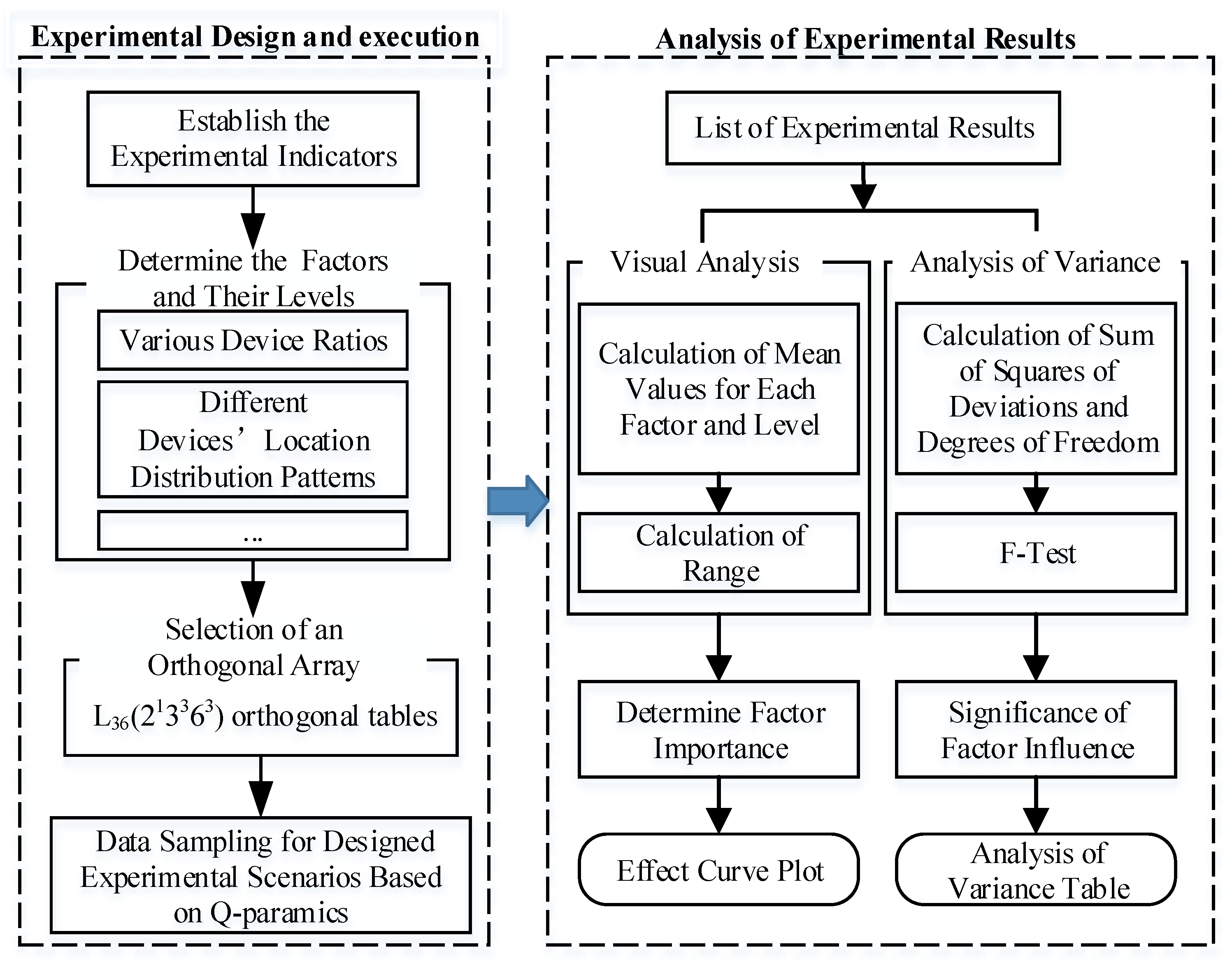
The experiment process consists of three parts: experimental design, experimental execution, and analysis of experimental results. The composition and relationships between the various parts are shown in Figure 1. For experimental design, six critical factors are considered. To account for the diverse data scenarios in real road networks, this paper proposes an orthogonal experimental design scheme. The utilization of L36(213363) orthogonal tables enables the creation of 36 scenarios, with each scenario meticulously repeated 10 times. The experiments were executed using data derived from each scenario utilizing the Q-paramics simulation software V6.8.1. The analysis of the experimental results entails both range analysis and variance analysis, providing a comprehensive evaluation of the data and drawing insightful conclusions.
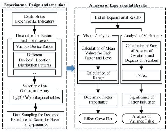
Figure 1.
Framework of the study.
3.2. Designing Orthogonal Experimental Scenarios Considering Complex Real-World Multisource Data Characteristics
The basic process of designing an orthogonal experimental plan includes the following steps: clarifying the experimental objectives, determining the experimental indicators, identifying the factors and their levels (i.e., different levels of the factors), selecting the orthogonal table, designing the table headers, and compiling the experimental plan. The purpose of this study is to analyze the factors affecting the accuracy of MFD construction under multisource data, providing guidance for the application of the proposed method in complex real-world scenarios. The experimental indicators are the root mean square errors between the MFD constructed under sampled data and the MFD constructed under all data, as detailed in Section 3.2.2. Below are the details for determining the experimental factors and levels, as well as the selection of the orthogonal table.
3.2.1. Design of Experimental Factor Levels
This paper considers six categories of factors that may influence the accuracy of MFD construction. These factors encompass the penetration rate of floating cars, the spatial distribution balance of floating cars, the coverage rate of fixed detectors, the spatial distribution pattern of fixed detectors, the recognition rate of license plate detectors, and the level of traffic demand. Considering the practical situation of traffic flow detection devices and their future development trends, the determination of the levels for each factor is expounded as follows.
- (1)
- Penetration Rate of Floating Cars ()
The penetration rate of floating cars refers to the proportion of floating cars among all vehicles in the road network [6]. In reference [14], it is pointed out that the only way to estimate the MFD without bias is to have the full information on vehicle trajectories over the network. However, it is difficult to obtain all the vehicle trajectories’ data. In this context, is pivotal in gauging the extent to which the selected floating car GPS data truly reflects the overall traffic characteristics within the study area. The levels for this factor are chosen based on the percentage of vehicles equipped with sensing devices, ranging from low to high levels of penetration. The penetration rate of floating cars for each origin-destination link signifies the proportion of floating cars within the total number of vehicles for that link. Considering the availability of floating car data in the road network and the future growth trend of floating cars, this study sets the floating car penetration rate at six levels: “0.05”, “0.1”, “0.15”, “0.2”, “0.25”, and “0.3”.
- (2)
- Spatial Distribution Balance of Floating Cars ()
In reference [18], the network flow and density were approximated by considering the proportion of probe vehicles as a constant value for all OD pairs. However, in actual road networks, the proportion of floating cars varies under different OD conditions. Furthermore, the spatial distribution balance of floating cars is crucial in understanding how well the sampled floating car’s characteristics represent the overall traffic patterns in the study area. The degree of balance in the spatial distribution reflects the difference in the travel characteristics between floating cars and the overall travel characteristics of the road network. The levels for this factor are determined by the degree of evenness in distributing floating cars across the road network, varying from uneven to highly balanced distribution. Based on the relative positions of the origin and destination traffic zones of floating car trips, this study classifies floating car trips into four categories: within-zone to within-zone, within-zone to outside-zone, outside-zone to within-zone, and outside-zone to outside-zone. The sum of the proportions of these four types of trips by floating cars amounts to 1. The spatial distribution balance of floating car GPS data is then assessed based on the Gini coefficient and the coverage levels. By varying the levels of coverage and spatial distribution equilibrium, the study can comprehensively investigate their impact on the accuracy of MFD construction. The Gini coefficient for calculating the spatial distribution of floating cars is expressed as Equation (1):
here, and , taking values 1, 2, 3, and 4, respectively, represent four types of trips: within-zone to within-zone, within-zone to outside-zone, outside-zone to within-zone, and outside-zone to outside-zone. denotes the Gini coefficient of floating car spatial distribution for the -th experimental scenario, used to assess the spatial distribution balance of floating cars. represents the proportion of floating cars in the total number of floating cars for the -th type of trips under the -th experimental scenario. signifies the average proportion of floating cars for each type of trip in the total number of floating cars under the -th experimental scenario.
- (3)
- Coverage Rate of Fixed Detectors ()
The fixed detectors’ coverage rate refers to the proportion of links equipped with fixed detectors among all links in the study area. In reference [12], it was concluded that a minimum detector coverage rate of 25% resulted in a difference of less than 15% between the partial and overall MFDs. On this basis, the variation in coverage rates, from low to high, portrays the current proportion of detectors and their ability to depict the overall traffic flow characteristics of the road network within the study area. Considering the diverse traffic management needs in different urban regions, this study establishes six levels of fixed detector coverage rate: “0.15”, “0.3”, “0.45”, “0.6”, “0.75”, and “0.9”.
- (4)
- Spatial Distribution Pattern of Fixed Detectors ()
The spatial distribution pattern of fixed detectors refers to the spatial arrangement of detectors on links at a specific fixed detector coverage rate. The differences in spatial distribution patterns represent the variations in how detectors are positioned and dispersed across the road network, indicating diverse arrangements and concentration levels. In reference [13], it is discovered that the distribution of loop detectors within the road network introduces significant deviations in MFD construction. To investigate how the spatial distribution pattern of fixed detectors affects MFD, this study classifies the spatial distribution pattern of fixed detectors into three levels: “random”, “clustered”, and “boundary”. In the “random” pattern, fixed detectors are distributed without any apparent regularity across the road network. In the “clustered” pattern, fixed detectors are predominantly concentrated in the central areas of the road network. In the “boundary” pattern, fixed detectors are positioned along the boundaries of the road network.
- (5)
- Recognition Rate of License Plate Detector ()
The recognition rate of the license plate detector represents the proportion of vehicles passing through the detector whose license plates are accurately identified. In this study, the license plate recognition devices are employed for link flow detection, the recognition rate plays a crucial role in link traffic flow detection, which influences the overall accuracy of the detection. Considering the current performance of both older and state-of-the-art license plate detectors, along with their potential future advancements, this study establishes the levels of license plate detector recognition rate at six discrete values: 0.75, 0.8, 0.85, 0.9, 0.95, and 1.
- (6)
- Traffic Demand Level ()
Considering future changes in traffic demand and their impact on the shape and dispersion of the MFD, it is necessary to analyze these factors to explore how variations in traffic demand affect the accuracy of MFD construction. The traffic demand level is systematically adjusted by proportionally expanding the traffic flow origin-destination (OD) through traffic simulation based on real traffic flow information. To explore different levels of traffic demand to analyze its impact on the MFD, the traffic demand level is established at three distinct levels: “100%”, “105%”, and “110%”, corresponding to the original traffic demand and incremental increases of 5% and 10% from the original demand, respectively.
3.2.2. Determination of Experimental Indicators
Continuing the methodology established in the previous thesis [1], the root mean square error between partial samples and full samples was selected as the accuracy evaluation index [28] and the calculation method is shown in Equation (2):
where is the root mean square error for the average traffic flow and average traffic density of the test site, and (vehs/h), respectively, donate the average traffic flow derived from simulated full-sample data and simulated multisource data during period, and (vehs/km) are average traffic density derived from simulated full-sample data and simulated multisource data during period, is the count of periods, (vehs/h) is the network traffic capacity, (vehs/km) is the maximum average traffic density, referring to the research of Saffari et al. [28], is approximated as the mean of the first three maximum average traffic densities.
3.3. Selection of Orthogonal Tables
The general form of an orthogonal table is denoted as , where stands for the number of experimental scenarios, represents the number of factor levels, and signifies the number of factors. Orthogonal tables are categorized into standard tables, nonstandard tables, and mixed orthogonal tables [27]. All the information for orthogonal tables is listed based on the number of factors and levels, which can be referred to whenever needed. When the factors require varying levels of examination or certain factors cannot have multiple levels, the use of mixed orthogonal tables is more suitable.
One of the principles of selecting orthogonal tables is to opt for the table with the fewest required experimental scenarios while adhering to the levels of the factors being tested. The second principle is to make sure the degrees of freedom of each factor and interaction effect are distributed relatively evenly, which can help to evaluate the flexibility and statistical power of experimental design. The degrees of freedom of an orthogonal table involve the flexibility of experimental design, which is related to the number of factors and levels in the experiment. Degrees of freedom refer to the number of independent elements in an experimental design that can be varied at will. From the perspective of degrees of freedom, the principle for selecting orthogonal tables is that the sum of single-factor degrees of freedom and error degrees of freedom should be less than the degrees of freedom of the orthogonal table. For instance, in a three-factor two-level experiment, L4(23) should be chosen, while for a five-factor two-level experiment, L8(27) should be preferred. Any unused columns can serve as error columns without affecting the experimental outcomes.
As depicted in the presentation of the experimental factors and their levels in Section 3.1, the experiment encompasses six factors, with three factors having six levels and three factors having three levels. Based on the principles of the orthogonal table selection, this study intends to employ the mixed orthogonal table L36(213363) to conduct orthogonal experiments. In this experiment, factors with the same levels can be arranged freely within the design, adhering to the chosen orthogonal table structure.
3.4. Analysis Method of Experimental Results
This section aims to employ the method of range analysis to assess the relative impact of each factor on the accuracy of MFD construction. The range signifies the difference between the maximum and minimum expected values of MFD construction errors across the levels of influencing factors. A larger range indicates a greater influence of that specific factor on the accuracy of MFD construction. The process of range analysis encompasses four components: data structuring and modeling, computation of effects for each factor at various levels, calculation of the range for the effects of each factor’s levels, and correction of the range in the context of mixed designs.
- (1)
- Modeling the Data Structuring
The foundation of range analysis lies in the model of experimental data structure and the effects of various factor levels. Effects are defined as the extent of influence that different factor levels have on experimental indicators, which is MFD construction errors in our study. Given that the levels of research factors are controllable, this study employs a fixed-effects model [27] to establish a relationship between MFD construction errors, the effects of different factor levels, and random errors. The model of the data structure in this paper is presented as follows.
The effects of factor at different levels are denoted as the set ; the effects of factor at different levels be represented as the set , the effects of factor at different levels be denoted as the set }, the effects of factor at different levels be expressed as the set , the effects of factor at different levels be defined as the set , and the effects of factor at different levels be described as the set , . represents the MFD construction error for a combination of factor levels. Considering the orthogonal table L36(213363), the data structure vector of the orthogonal table is illustrated by Equation (3):
where represents the MFD construction error for each combination of factor levels, embodies the overall influence of various factor level combinations on the experimental indicator , denote the effects of the respective factor levels for the th experimental scenario, where , signifies the number of experimental scenarios, stands for the experimental error of the th experimental scenario, which, in the absence of systematic error, follows a normal distribution . Here, represents the overall variance of MFD construction errors across all experimental scenarios.
It should be noted that the effects of factors adhere to the principle wherein the summation of effects for various levels of the same factor equals zero, as illustrated in Equation (4).
- (2)
- Computation of Effects for Factor Level
Based on the previously established data structure model between the MFD construction errors and the effects of various factors for each experimental scenario, it is feasible to estimate the overall impact of various factor-level combinations on the accuracy of MFD construction as well as the influences of individual factors. The model’s estimation is achieved through the incorporation of observed MFD construction error values. Note the collection of MFD construction errors for each experimental scenario as with elements , as the MFD construction error of the th experimental scenario. The estimation objective of the model () is to minimize the disparity between the experimental outcomes of MFD construction errors across different experimental scenarios and the model’s estimated results [29]. The estimation objective is illustrated in the form of the objective function given in Equation (5)
where denotes the MFD construction error for the th experimental scenario and and carry the same meaning as in Equation (3).
The overall impact of various factor-level combinations on the experimental indicator can be achieved by employing the least squares method [30] through solving the structural model parameters. The overall impact is . The effects of different factor levels are denoted as , . Here, the mean of the experimental indicator at each factor level, , is computed using Equation (6)
where, represents the MFD construction error for the th experimental scenario, stands for the mean MFD construction error for the th factor at the th level, signifies the set of experimental scenarios for the th factor at the th level, and denotes , i.e., the number of elements in the set of experimental scenarios .
- (3)
- The Calculation of Range for Factor Levels’ Effects
Based on the average MFD construction errors (or effect values) at different factor levels, the calculation of the range is presented in Equation (7):
where, h is the number of levels for the th factor, represents the range of effects of the MFD construction error for the various levels of the th factor before correction, and signifies the mean MFD construction error for the th factor at the level.
- (4)
- The Rectification of Range for Mixed-Level Design
When the factor levels in an orthogonal design are the same, the prioritized relationship of factors can be determined through the range of extreme values. Given the variation in the levels of various influencing factors, the mixed-level table L36(213363) is employed for range analysis in our study. Under mixed-level conditions, factors with more diverse levels may exhibit greater variability in range (i.e., scope of variation), which influences the precision of assessing the impact of the factors’ levels. Therefore, it becomes necessary to rectify the range of the mixed-level experiment. The specific rectification approach involves multiplying the range of each factor in the experiment by the corresponding correction coefficient based on the factor levels [27]. Table 1 presents the range rectification table for the mixed-level experiment and the specific rectification method is depicted in Equation (8)
where, and represent the range before and after rectification of the mixed-level experiment, respectively, signifies the number of levels, and stands for the range correction coefficient for the factor under level .

Table 1.
Coefficients for range rectification.
- (5)
- Analysis of Variance
Building upon the computed effects of key influencing factors and their levels, as determined in the preceding sections, a significance analysis known as an analysis of variance (ANOVA) on all factors influencing the precision of the MFD constructions was undertaken utilizing F-tests. Variance analysis [27] stands as one of the fundamental techniques in mathematical statistics. It employs the manifestation of data fluctuations (variations) to signify the impact of a specific factor or stochastic error. The study further employs the F-test to ascertain the significance of this impact. The general process of variance analysis encompasses the computation of the sum of the squared deviations, the determination of the degrees of freedom, and the application of the F-test.
In this manuscript, the total sum of the squared deviations in the orthogonal table is employed to represent the overall variability of the MFD construction errors. Likewise, the sum of the squared deviations for each column signifies the variability of the MFD construction errors caused by the variation in the levels within that column of the orthogonal table. Notably, the sum of the squared deviations for the empty columns refers to the variability induced by the experimental errors and unexamined factors. The methodologies for calculating the total sum of the squared deviations and the sum of the squared deviations for each column are elucidated through Equations (9) and (10), respectively.
where, represents the total sum of the squared deviations between the MFD construction errors for all scenarios in the orthogonal table and their overall mean value, signifies the sum of the squared deviations between the average MFD construction error at the -th factor level and the overall mean value, stands for the mean value of the MFD construction errors across all scenarios, denotes the number of levels for the -th factor, represents the mean value of the MFD construction errors corresponding to the -th level of the -th factor, stands for the number of experimental scenarios, and denotes the MFD construction error for the -th experimental scenario.
The total sum of the squared deviations (or its corresponding degrees of freedom) is equal to the sum of the squared deviations (or corresponding degrees of freedom) attributable to individual factors, interaction effects, and empty columns that influence the precision of the MFD construction. The sum of the squared deviations for the empty columns typically represents the squared deviations due to experimental errors. The methodologies for calculating the total sum of the squared deviations and the corresponding degrees of freedom are presented in Equation (11) and Equation (12), respectively.
where represents the degrees of freedom corresponding to the total sum of squared deviations, signifies the degrees of freedom for the -th factor, denotes the number of factors in the orthogonal table, and and have the same meanings as in Equation (9).
Based on the sum of squared deviations and degrees of freedom attributed to factors influencing the precision of MFD constructions, the F-test methodology facilitates the analysis of significance for each factor. Taking the fixed pattern of vehicle detector spatial distribution factor () as an example, with corresponding levels of effects denoted as and = , the null hypothesis for the F-test is presented as Equation (13)
where, , and represent the effects at the various levels of factor .
If is true, it indicates that the fixed pattern of vehicle detector spatial distribution has no significant impact on the precision of MFD construction. The sum of the squared deviations for this factor is influenced solely by experimental errors and its mean square serves as an unbiased estimate of the total variance of MFD construction errors across all experimental scenarios. Similarly, using the example of the factor , the F-test statistic is calculated as shown in Equation (14)
where, is an F-distributed random variable with degrees of freedom , representing the F-ratio for the factor , denotes the sum of squared deviations for the factor , signifies the degrees of freedom for the experimental error term, stands for the sum of squared deviations of the experimental error term, and and , respectively, represent the sample variances of the factor and the error term.
At the chosen significance level , the critical value can be obtained from the F-distribution table. For a given experiment, if exceeds , the null hypothesis is rejected. Consequently, it is concluded that at the significance level , the varying levels of the factor significantly affect the MFD construction errors. It is noteworthy that if the sum of squared deviations for individual factors within the experiment is relatively small, it can be combined with the sum of squared deviations for the error column to form the sum of squared deviations for experimental errors. In this case, the corresponding degrees of freedom are also combined.
4. Results
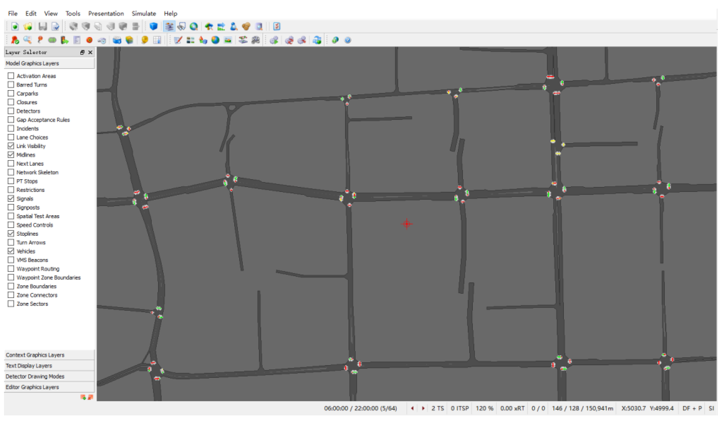
In view of the difficulty of evaluating the accuracy of the proposed method based on real traffic data, the actual traffic of the test site was simulated based on Q-paramics simulation software V6.8.1. The road network of approximately 2.4 km2 in the central urban area of Kunshan City, China, was selected as the test site. The road network consists of 71 road segments and 18 intersections, including frequently congested roads and intersections such as Qianjin Road, Bailu Road, and Zhenchuan Road. The simulated road network, as shown in Figure 2, aligns with the actual network. Based on the traffic flow data of links and intersections that can be observed in 15 min, this paper refers to the method of the literature [31] to calibrate parameters such as traffic demand and the link’s traffic capacity for traffic simulation. The start time of the simulation is 06:00:00 and the duration is 16 h. The simulation settings are consistent with those in previous research [1]; encompassing aspects such as road network, traffic demand, and signal control, we simulate and subsequently analyze traffic flow data for various experimental scenarios.
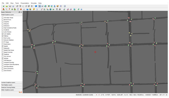
Figure 2.
The road network of test site for simulation.
To be more specific, in Section 4.1, the traffic simulation is set up to output comprehensive trajectory data and link traffic flow data. Based on the experimental scenarios defined in Section 3, sampled trajectory data and link traffic flow data are generated according to the defined levels of various factors for the experimental scenarios. And then, the MFD is constructed using multisource data. The evaluation of the influencing factors and their respective significance levels for MFD construction in different data scenarios is conducted through the calculation of RMSE (root mean square error).
4.1. Data Sampling for Various Experimental Scenarios Based on Traffic Simulation
The sampling process for floating car data based on traffic simulation involves various steps, including inputting experimental scenarios, determining the penetration rate, determining the proportions of different types of floating cars to represent spatial distribution patterns, and outputting sampled floating car data. The specific steps are outlined in Table 2. Initially, the total count of floating cars within the entire vehicle population is determined based on the provided penetration rate of floating cars. Subsequently, four random sampling proportions, summing to 1, are generated. These correspond to different proportions of floating cars in various types of traffic zones. The Gini coefficient with different levels is utilized to gauge the balance degree of different proportions across different traffic zone. On this basis, the sampled floating cars’ distribution pattern can be aligned with the current experimental design. Next, samples are drawn from different types of traffic zones based on the four sampling proportions while maintaining a constant total count of floating car samples. Finally, all samples are determined and their vehicle trajectory data are outputted. It is worthy noting that in this study, “within the region” refers to floating cars with origin or destination points within the study area while “outside the region” indicates floating vehicles with origin or destination points outside the study road network and within the region bounded by the inner ring road of Kunshan [1].
Table 2.
Sampling process for floating car data.
The sampling process for link traffic flow data using fixed detectors through traffic simulation involves several steps, including inputting experimental scenarios, determining the coverage rate of fixed detectors, selecting sets of fixed detectors with different spatial distribution patterns under varying coverage rates, and outputting sampled link traffic flow data. First, determine the total count of fixed detectors. Based on the total number of links in the simulation road network (all links equipped with fixed detectors), calculate the total count of sampled fixed detectors according to the coverage rate specified in the experimental scenario. Second, determine the samples of fixed detectors based on spatial distribution patterns. Maintaining the total count of fixed detectors, sample a certain quantity of fixed detectors based on the chosen spatial distribution pattern. For the “Random” pattern, perform random sampling. For the “Cluster” and “Boundary” patterns, determine the set of detectors closest or farthest from the center of the test site. Finally, determine the set of fixed vehicle detectors and output the link traffic flow data. The specific steps for sampling link traffic flow data based on fixed detectors are provided in Table 3.
Table 3.
Link traffic flow data sampling based on traffic simulation.
4.2. Experimental Results
Based on the orthogonal experimental design method proposed earlier, the MFD using sampled vehicle trajectory data and sampled link traffic flow data utilizing traffic simulation is constructed. The root mean square error (RMSE) is computed between MFD constructed using sampled data and MFD constructed using the entire data. The orthogonal experimental design plan and results are presented in Table 4.
Table 4.
L36(213363) orthogonal table.
An analysis of the MFD construction errors across different scenarios in Table 4 reveals the following patterns:
First, when the fixed detector coverage exceeds 45%, the penetration rate of floating cars is above 10%, and the spatial distribution of floating cars is either “moderate” or “strong” (as seen in scenarios 2, 3, 4, 5, 8, 11, 21, and 22), the median error in MFD construction is similar (around 8~10%). This is because, in such scenarios, the representativeness of vehicle trajectory data is comparable, allowing for a more accurate estimation of the MFD.
Second, when the fixed detector coverage is below 30%, the penetration rate of floating cars is less than 15%, and the spatial distribution of floating cars is mostly “weak” (as seen in scenarios 1, 13, 16, 17, 28, 33, and 36), the median error in MFD construction is relatively high (around 10~20%). This may be due to significant differences between the travel characteristics of the floating car samples and the overall vehicle population in such scenarios, leading to larger estimation errors in the MFD.
4.3. Analysis of Experimental Results
- (1)
- Range Analysis for Experimental Results
Figure 3 illustrates the results of the range analysis. On the graph, the horizontal axis represents the levels of each factor while the vertical axis represents the root mean square error (RMSE) of errors between the MFD using sampled data and the MFD based on entire data.

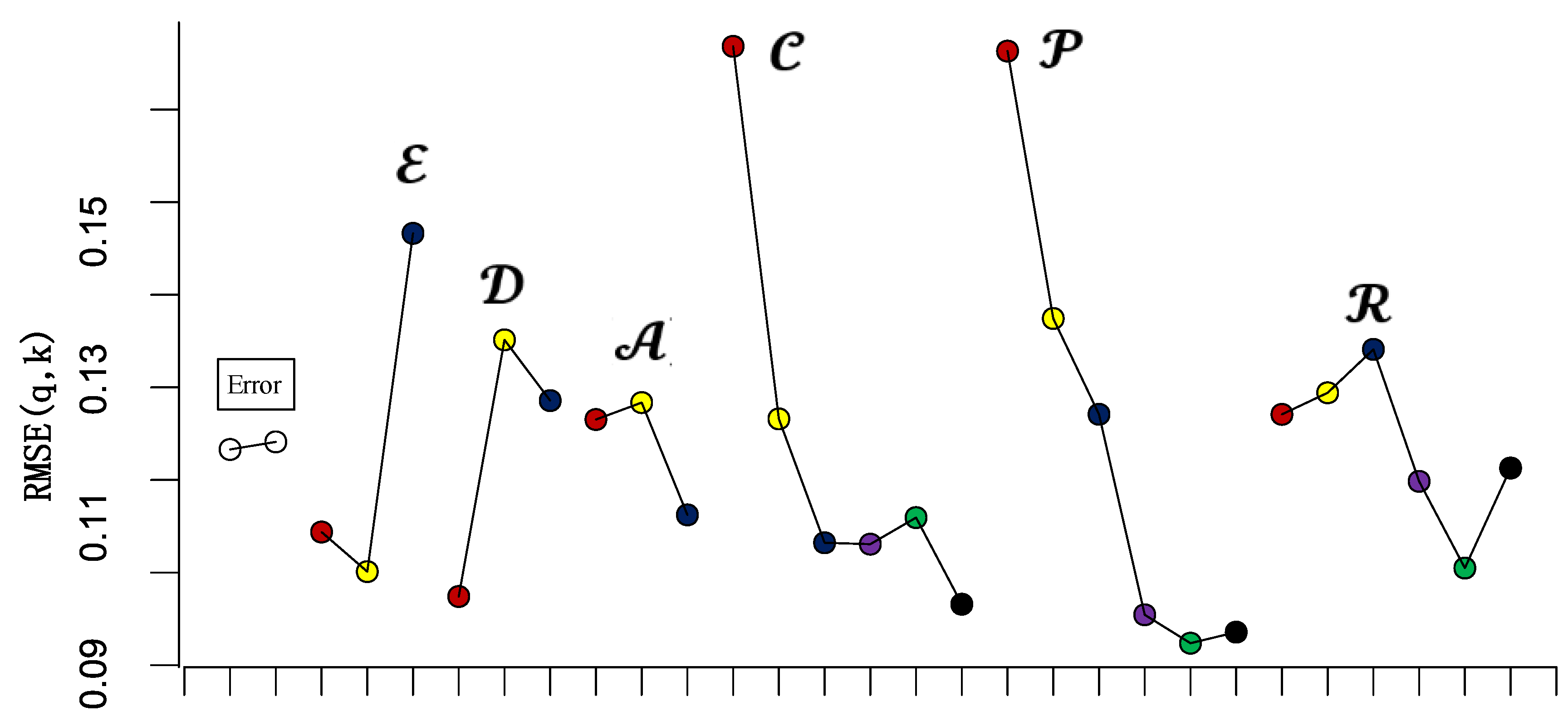
Figure 3.
Average error of MFD construction for each factor level.
In the figure, represents the factors, with meanings consistent with Section 3.2. The solid dots in red, yellow, blue, purple, green, and black correspond to the average MFD construction errors at the first, second, third, fourth, fifth, and sixth levels of each factor, respectively.
For each factor, a larger RMSE under different levels indicates a greater impact of that factor on the accuracy of MFD construction. Considering the use of the mixed orthogonal table L36(213363) in this study, where the number of levels for each factor varies, adjustments were made to rectify the ranges of experimental indicators corresponding to different levels of each factor. Figure 3 presents the results before these adjustments.
From the graph, it is evident that the RMSE range for different levels of fixed detectors’ coverage rate and floating cars’ penetration rate is notably larger than that of other factors. The RMSE range for floating cars’ spatial distribution equilibrium is comparatively smaller. After rectifying the RMSE ranges for each factor, the order of impact on MFD construction accuracy, based on the magnitude of adjusted ranges, is as follows: floating cars’ spatial distribution equilibrium (adjusted range value: 0.0666), fixed detectors’ coverage rate (adjusted range value: 0.0598), floating cars’ penetration rate (adjusted range value: 0.0580), traffic demand level (adjusted range value: 0.0504), license plate detectors’ recognition rate (adjusted range value: 0.0218), and fixed detectors’ spatial distribution pattern (adjusted range value: 0.0216). After rectification, the RMSE ranges for different levels of floating cars’ spatial distribution equilibrium shows a noticeable increase.
Based on this analysis, the critical influencing factors in this study are floating cars’ spatial distribution equilibrium (), fixed detectors’ coverage rate (), floating cars’ penetration rate (), and traffic demand level ().
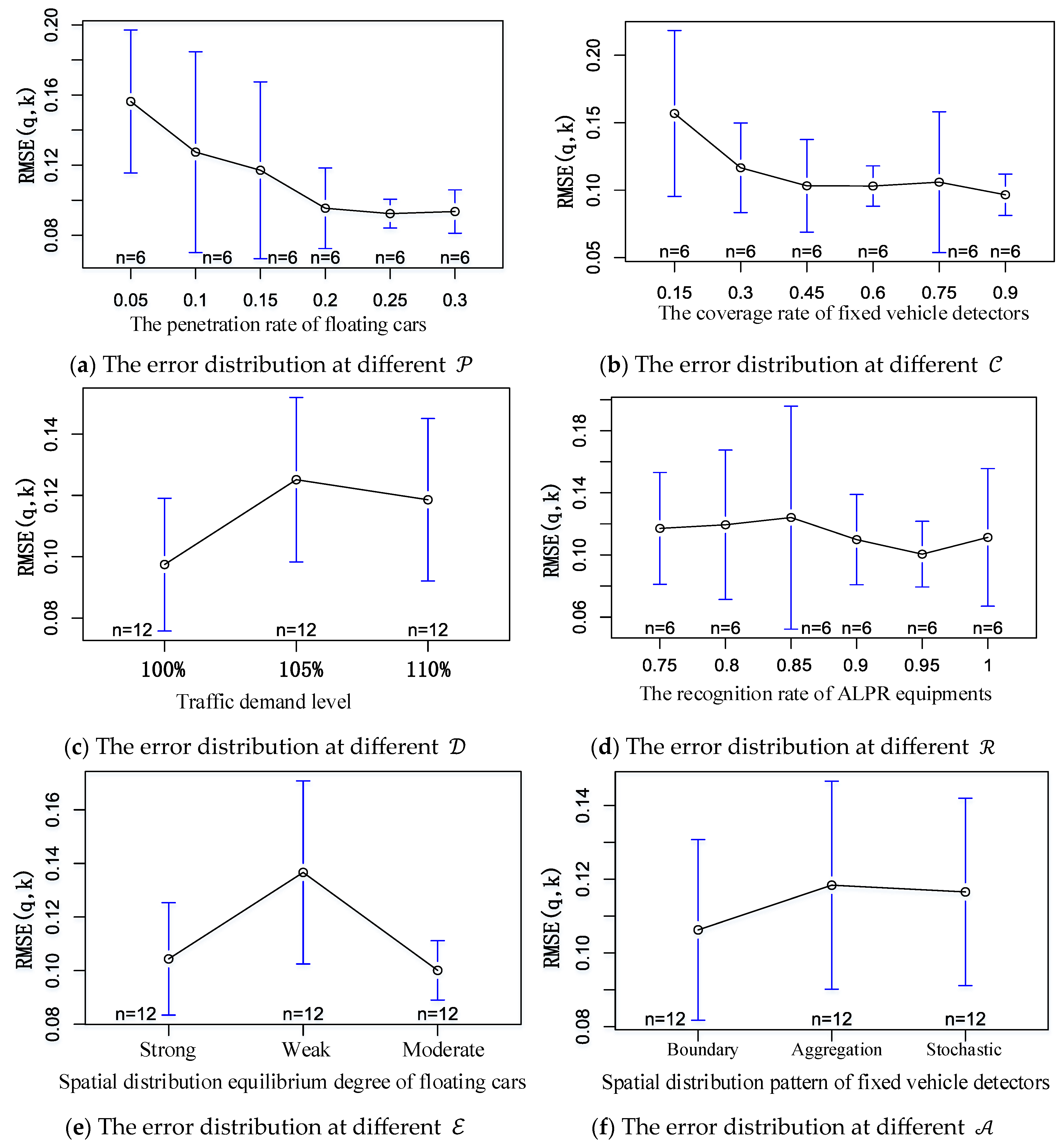
Figure 4 illustrates the error distribution results between the MFD using sampled data and the MFD based on entire data under different levels of each factor. In the graphs, the horizontal axis represents the levels of each factor, while the vertical axis depicts the error distribution for MFD under the respective factor levels. It is worth noting that, in the figure, n represents the number of trials for a specific factor level in a single experiment. The similarities or differences of n for different factors depend on the type of orthogonal table used. Since this study employs a mixed orthogonal table, the factor levels vary.
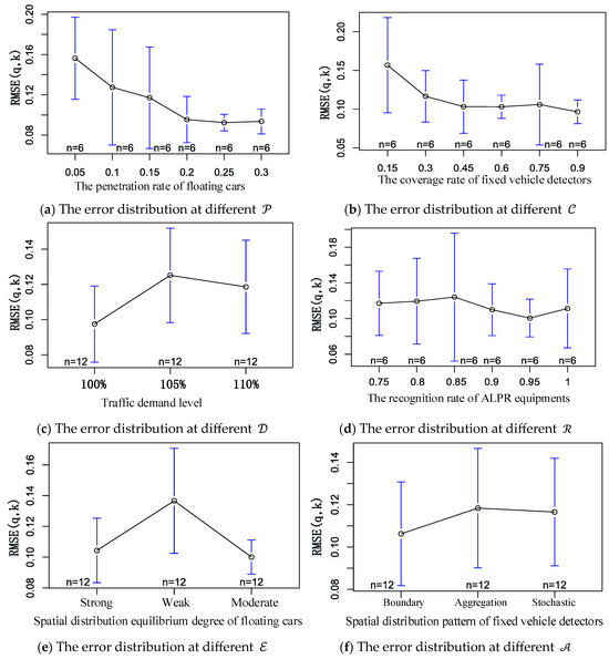
Figure 4.
The error distribution for each factor level in the experiment with orthogonal table L36(213363).
Figure 4a demonstrates the error distribution at different penetration rates of floating cars, it can be observed that as the floating car penetration rate increases, the error gradually diminishes. After the penetration rate reaches 20%, the median error remains approximately around 10%. This could be attributed to the proposed method accounting for varying penetration rates across different origin-destination links. When the overall penetration rate reaches 20%, the spatial distribution structure of vehicle trips in the road network is accurately captured.
Figure 4b demonstrates the error distribution at different coverage rates of fixed vehicle detectors, it reveals that the median error decreases with higher fixed detectors’ coverage rate. Once the coverage rate surpasses 45%, the error stabilizes at around 10%. This can be attributed to the different coverage of crucial road links (such as primarily main and secondary roads) by fixed detectors at the current coverage level.
Figure 4c demonstrates the error distribution at different traffic demand levels, it showing varying median error estimates for different levels of traffic demand. This variation arises because the study magnifies actual road network traffic demand proportionally (e.g., 105% indicates a 5% increase over the calibrated traffic demand). The increase in overall traffic demand intensifies congestion, impacting route choice behavior and subsequently altering traffic demand distribution patterns.
Figure 4d demonstrates the error distribution at different recognition rates of ALPR equipment; it indicates relatively minor differences in median error estimates for different license plate detector recognition rates. This could stem from the alignment of floating car license plate recognition rates with the overall recognition rate.
Figure 4e demonstrates the error distribution at different equilibrium degrees of spatial distribution of floating cars. It reveals that when the floating vehicle spatial distribution equilibrium is “weak”, the median error in MFD construction notably increases. This is due to the significant divergence between the travel characteristics of samples of floating cars and the overall travel characteristics of vehicles in the road network.
Lastly, Figure 4f demonstrates the error distribution at different spatial distribution pattern of fixed vehicle detectors. It depicts minimal differences in median error estimates for different fixed detectors’ spatial distribution patterns. This might result from the relatively small road network used in this study, which limits the depiction of variations in different fixed detectors’ spatial distribution patterns.
- (2)
- Variance Analysis for Experimental Results
While range analysis provides a preliminary exploration of the influence of different factor levels on experimental indicators within orthogonal experiments, it doesn’t distinguish whether the errors under different factor levels are attributed to the factor levels themselves or random errors. To ascertain whether the effects are due to random errors, a variance analysis is performed on the experimental results. The results of the variance analysis are summarized in Table 5.
Table 5.
The experimental results analysis for variance with orthogonal table l36(213363).
The variance analysis results in Table 5 include the degrees of freedom (Df) for each factor, the sum of squared deviations (Sum Sq) of experimental indicators under each factor, the mean squared deviations (Mean Sq) for experimental indicators at each factor level (calculated by dividing the sum of squared deviations by the degrees of freedom for that factor), the F-value for each factor (F value), the probability of F-ratios for each factor being less than (Pr(>F)), and the significance level ().
From Table 5, it is evident that within the orthogonal experiment, the factors influencing the construction accuracy of MFD include floating cars’ spatial distribution equilibrium, fixed detectors’ coverage rate, floating cars’ penetration rate, and traffic demand level. The results of the variance analysis indicate that the construction error of the MFD is indeed caused by variations in the levels of the factors. These findings align with the results obtained from the earlier range analysis.
5. Conclusions and Discussion
This study represented a valuable attempt to apply experimental analysis techniques to the examination of MFD influencing factors, providing new insights for future related research. In addition, it offers practical guidance for constructing MFDs in real-world road networks characterized by diverse and complex data scenarios.
In the study, six factors are considered in the experiment: floating cars’ penetration rate, floating cars’ spatial distribution equilibrium, fixed detectors’ coverage rate, fixed detectors’ spatial distribution pattern, license plate detection devices’ recognition rate, and traffic demand level. The experiment was performed using the L36(213363) orthogonal table and the results were analyzed through range analysis and variance analysis.
The analysis of the factors influencing the accuracy of MFD construction under different scenarios demonstrate the following conclusions: First, the influencing factors on MFD construction accuracy, ranked by their impact magnitude, are as follows: floating cars’ spatial distribution equilibrium, fixed detectors’ coverage rate, floating cars’ penetration rate, traffic demand level. Second, when the penetration rate reaches 20%, the error remains approximately around 10%. Third, once the coverage rate surpasses 45%, the errors stabilize at around 10%. Fourth, when the fixed detector coverage exceeds 45%, the penetration rate of floating cars is above 10%, and the spatial distribution of floating cars is either “moderate” or “strong”, the median error in MFD construction is around 8~10%. Finally, when the fixed detector coverage is below 30%, the penetration rate of floating cars is less than 15%, and the spatial distribution of floating cars is mostly “weak”, the median error in MFD construction is around 10~20%.
Theoretically, based on the above results, it can be observed that with a single data source, the MFD construction error can be maintained at a relatively low level (10%) when the fixed detector coverage reaches 45% or the floating car penetration rate exceeds 20%. With multisource data, to maintain the same error level, the required floating car penetration rate or fixed detector coverage can be reduced by approximately 10%, provided that the spatial distribution uniformity of the floating cars remains at a moderate or higher level.
Practically, since the road network data, OD data, and signal control information used in this study are all derived from real data (from the urban area of Kunshan, China), the research findings can guide detector placement as well as data collection scope and granularity for regional traffic control and congestion charging based on MFD in small to medium-sized cities with similar characteristics. However, due to the greater heterogeneity of traffic flow distribution in larger cities, broader applications in such urban areas may require additional data testing to validate their applicability.
Given the limitations of time and resources, this study requires further in-depth exploration. Specifically, future research could be developed in the following two directions: (1) establishing a relationship model between influencing factors and the accuracy of MFD construction to study how to estimate MFD construction errors based on existing multisource data characteristics and (2) further applying the conclusions of this study, such as in threshold control, and assessing the reliability of the proposed methods based on the control results.
Funding
This work is sponsored by Natural Science Foundation of Xinjiang Uygur Autonomous Region (No. 2022D01C691) and the Tianchi Talent Recruitment Plan of Xinjiang Uygur Autonomous Region.
Institutional Review Board Statement
Not applicable.
Informed Consent Statement
Not applicable.
Data Availability Statement
The data presented in this study are available on request from the first author. The data are not publicly available due to licensing restrictions from data providers.
Conflicts of Interest
The authors declare no conflict of interest.
References
- Hong, R.; Liu, H.; An, C.; Wang, B.; Lu, Z.; Xia, J. An MFD construction method considering multi-source data reliability for urban road networks. Sustainability 2022, 14, 6188. [Google Scholar] [CrossRef]
- Zhang, L.; Yuan, Z.; Yang, L.; Liu, Z. Recent developments in traffic flow modelling using macroscopic fundamental diagram. Transp. Rev. 2020, 40, 689–710. [Google Scholar] [CrossRef]
- Daganzo, C.F.; Geroliminis, N. An analytical approximation for the macroscopic fundamental diagram of urban traffic. Transp. Res. Part B Methodol. 2008, 42, 771–781. [Google Scholar] [CrossRef]
- Buisson, C.; Ladier, C. Exploring the impact of homogeneity of traffic measurements on the existence of macroscopic fundamental diagrams. Transp. Res. Rec. J. Transp. Res. Board 2009, 2124, 127–136. [Google Scholar] [CrossRef]
- Cassidy, M.J.; Jang, K.; Daganzo, C.F. Macroscopic Fundamental Diagrams for Freeway Networks: Theory and Observation. In Proceedings of the Transportation Research Board (TRB) 2011 Annual Meeting, Washington, DC, USA, 23–27 January 2011; Volume 2260, pp. 8–15. [Google Scholar]
- Ma, Y. Research on Traffic Control Strategies for Traffic Communities. Master’s Thesis, Tongji University, Shanghai, China, 2010. [Google Scholar]
- Xu, F.; He, Z.; Sha, Z. Impacts of traffic management measures on urban network Microscopic Fundamental Diagram. J. Transp. Syst. Eng. Inf. Technol. 2013, 13, 189–194. [Google Scholar]
- Zhang, L.; Garoni, T.M.; Gier, J.D. A comparative study of Macroscopic Fundamental Diagrams of arterial road networks governed by adaptive traffic signal systems. Transp. Res. Part B Methodol. 2013, 49, 1–23. [Google Scholar] [CrossRef]
- Johari, M.; Keyvan-Ekbatani, M.; Leclercq, L.; Ngoduy, D.; Mahmassani, H.S. Macroscopic network-level traffic models: Bridging fifty years of development toward the next era. Transp. Res. Part C Emerg. Technol. 2021, 131, 103334. [Google Scholar] [CrossRef]
- Ma, W.; Liao, D. Process and Prospects of Macroscopic Fundamental Diagram. J. Wuhan Univ. Technol. (Transp. Sci. Eng. Ed.) 2014, 38, 1226–1233. [Google Scholar]
- Geroliminis, N.; Sun, J. Properties of a well-defined macroscopic fundamental diagram for urban traffic. Transp. Res. Part B Methodol. 2011, 45, 605–617. [Google Scholar] [CrossRef]
- Ortigosa, J.; Menendez, M.; Tapia, H. Study on the number and location of measurement points for an MFD perimeter control scheme: A case study of Zurich. EURO J. Transp. Logist. 2014, 3, 245–266. [Google Scholar] [CrossRef]
- Courbon, T.; Leclercq, L. Cross-comparison of macroscopic fundamental diagram estimation methods. Procedia-Soc. Behav. Sci. 2011, 20, 417–426. [Google Scholar] [CrossRef]
- Leclercq, L.; Chiabaut, N.; Trinquier, B. Macroscopic fundamental diagrams: A cross-comparison of estimation methods. Transp. Res. Part B Methodol. 2014, 62, 1–12. [Google Scholar] [CrossRef]
- Lee, G.; Ding, Z.; Laval, J. Effects of loop detector position on the macroscopic fundamental diagram. Transp. Res. Part C Emerg. Technol. 2023, 154, 104239. [Google Scholar] [CrossRef]
- Rizvi, S.M.A. Framework for the Selection of Loop Detectors for Macroscopic Fundamental Diagram Estimation. EasyChair 2023, 10424. [Google Scholar] [CrossRef]
- Geroliminis, N.; Daganzo, C.F. Existence of urban-scale macroscopic fundamental diagrams: Some experimental findings. Transp. Res. Part B Methodol. 2008, 42, 759–770. [Google Scholar] [CrossRef]
- Nagle, A.S.; Gayah, V.V. Accuracy of Networkwide Traffic States Estimated from Mobile Probe Data. Transp. Res. Rec. J. Transp. Res. Board 2014, 2421, 1–11. [Google Scholar] [CrossRef]
- Tilg, G.; Pawlowski, A.; Bogenberger, K. The impact of data characteristics on the estimation of the three-dimensional passenger macroscopic fundamental diagram. In Proceedings of the 2021 IEEE International Intelligent Transportation Systems Conference (ITSC), Indianapolis, IN, USA, 19–22 September 2021; IEEE: New York, NY, USA; pp. 2111–2117. [Google Scholar]
- Du, J.; Rakha, H.; Gayah, V.V. Deriving macroscopic fundamental diagrams from probe data: Issues and proposed solutions. Transp. Res. Part C Emerg. Technol. 2016, 66, 136–149. [Google Scholar] [CrossRef]
- Saffari, E.; Yildirimoglu, M.; Hickman, M. Estimation of macroscopic fundamental diagram solely from probe vehicle trajectories with an unknown penetration rate. IEEE Trans. Intell. Transp. Syst. 2023, 24, 14970–14981. [Google Scholar] [CrossRef]
- Ambühl, L.; Menendez, M. Data fusion algorithm for macroscopic fundamental diagram estimation. Transp. Res. Part C Emerg. Technol. 2016, 71, 184–197. [Google Scholar]
- Min, J.H.; Ham, S.W.; Kim, D.K.; Lee, E.H. Deep multimodal learning for traffic speed estimation combining dedicated short-range communication and vehicle detection system data. Transp. Res. Rec. 2023, 2677, 247–259. [Google Scholar] [CrossRef]
- Ji, Y.; Xu, M.; Li, J.; Van Zuylen, H.J. Determining the macroscopic fundamental diagram from mixed and partial traffic data. Promet-Traffic Transp. 2018, 30, 267–279. [Google Scholar] [CrossRef]
- Fu, H.; Wang, Y.; Tang, X.; Zheng, N.; Geroliminis, N. Empirical analysis of large-scale multimodal traffic with multi-sensor data. Transp. Res. Part C Emerg. Technol. 2020, 118, 102725. [Google Scholar] [CrossRef]
- Jiang, H. An Application Study of Orthogonal Experiment on Improving Color Difference of Cell Phone in Painting Process. Master’s Thesis, School of Mechanical Engineering of Shanghai Jiaotong University, Shanghai, China, 2007. [Google Scholar]
- Ren, L. Experimental Optimization Design and Analysis; Higher Education Press: Beijing, China, 2003; pp. 79–102. [Google Scholar]
- Saffari, E.; Yildirimoglu, M.; Hickman, M. A methodology for identifying critical links and estimating macroscopic fundamental diagram in large-scale urban networks. Transp. Res. Part C Emerg. Technol. 2020, 119, 102743. [Google Scholar] [CrossRef]
- Geng, Y.; Bu, X.; Wei, X. The calculation of effect and the anticipant estimation of target’s value in upright overlapping design of experiment. J. Hebei Inst. Archit. Civ. Eng. 2001, 4, 51–54+57. [Google Scholar]
- Chen, K. Experimental Design and Analysis, 2nd ed.; Tsinghua University Press: Beijing, China, 2005; pp. 72–136. [Google Scholar]
- Nie, Q. On-Line Estimation of Dynamic OD Flows for Urban Road Networks Based on Traffic Propagation Characteristic Analysis. Ph.D. Thesis, Southeast University, Nanjing, China, 2017. [Google Scholar]
Disclaimer/Publisher’s Note: The statements, opinions and data contained in all publications are solely those of the individual author(s) and contributor(s) and not of MDPI and/or the editor(s). MDPI and/or the editor(s) disclaim responsibility for any injury to people or property resulting from any ideas, methods, instructions or products referred to in the content. |
© 2024 by the author. Licensee MDPI, Basel, Switzerland. This article is an open access article distributed under the terms and conditions of the Creative Commons Attribution (CC BY) license (https://creativecommons.org/licenses/by/4.0/).