Extraction of Maize Distribution Information Based on Critical Fertility Periods and Active–Passive Remote Sensing

Abstract

This study proposes a new method for integrating active and passive remote sensing data during critical reproductive periods in order to extract maize areas early and to address the problem of low accuracy in the classification of maize-growing areas affected by climate change. Focusing on Jiaozuo City, this study utilized active–passive remote sensing images to determine the optimal time for maize identification. The relative importance of features was assessed using a feature selection method combined with a machine learning algorithm, the impact of both single-source and multi-source features on accuracy was analyzed to generate the optimal feature subset, and the classification accuracies of different machine learning classification methods for maize at the tasseling stage were compared. Ultimately, this study identified the most effective remote sensing features and methods for maize detection during the optimal fertility period. The experimental results show that the feature set optimized for the tasseling stage significantly enhanced maize recognition accuracy. Specifically, the random forest (RF) method, when applied to the multi-source data fusion feature set, yielded the highest accuracy, improving classification accuracy by 24.6% and 4.86% over single-source features, and achieving an overall accuracy of 93.38% with a Kappa coefficient of 0.91. Data on the study area’s maize area were also extracted for the years 2018–2022, with accuracy values of 93.83%, 98.77%, 97%, and 98.05%, respectively.

1. Introduction

As one of the three main grain crops grown in China, maize accounted for 37.17% of the planted area and 41.54% of the total output of all grain crops in 2023. Planning for the import and export of agricultural products, controlling the agricultural structure, and guaranteeing food security all depend on the timely and efficient identification of maize planting areas [1,2].

With the rapid development of remote sensing technology, the extraction of crop areas using remote sensing has become a prominent field in agricultural remote sensing [3]. Using various techniques to completely realize the spectral, phenological, and textural distinctions between crops and other surface cover types is the fundamental goal of crop extraction [4,5]. Optical satellite remote sensing data play a crucial role in crop extraction technology, but they are easily affected by cloudy and rainy weather [6]. Collecting feature information during the rainy season when the cloud cover is severe or the soil moisture is high does not affect the resulting SAR data [7,8,9,10]. In addition, Sentinel-1 SAR data have been used in studies involving flood monitoring, crop yield estimation, and waterbody extraction [11,12], and the results validate the use of SAR data for land-use classification. Combining optical and radar satellite remote sensing data can improve crop identification accuracy [13,14].

Accurate crop area and spatial distribution information is critical for estimating crop parameters and predicting yields. Crop identification, as the initial stage of precision agriculture, plays a vital role in ensuring food security, supporting economic development, and guiding the formulation of agricultural policies at all levels of government. The timely, accurate, and comprehensive monitoring of crop types and areas is therefore essential. Early extraction of cultivated areas, before crops reach maturity, offers several advantages. By conducting pre-harvest risk assessments, the agricultural insurance sector can dynamically adjust policies based on the evolving risk landscape, providing more flexible and targeted protection. Furthermore, early identification allows for the timely detection of potential disaster risks, such as pests, diseases, droughts, and floods, enabling the implementation of preventive measures.

Currently, remote sensing technology for maize area extraction primarily focuses on two approaches: (1) maize area identification methods that are based on imagery from a single phenological period or a specific date, and (2) identification methods that utilize individual features across multiple phenological periods. However, relying on a single seasonal period does not allow for the entire reproductive cycle of maize to be adequately captured. In addition, factors such as rainy weather can adversely impact both crop growth and the quality of remote sensing images, thus affecting extraction accuracy. While constructing a time series to extract crop areas—spanning the entire reproductive period from sowing to harvest—provides a more comprehensive view, it often leads to delays in area extraction, preventing timely assessments when needed. Ma et al. [15] integrated SAR data with optical data, utilizing polarization and spectral information to improve the overall accuracy of wheat classification, but the study only focused on a single wheat greening period. Wu et al. [16] compared different phenological periods and classification methods and found that the overall classification accuracy of the multi-phenological characteristic index of random forests was higher. However, the study only used eight optical data features. Liu et al. [17] used the random forest method and found that winter wheat was best separated from other land cover types during the jointing–heading period, but the study was only based on optical data. In a study of maize classification, Lv et al. [18] used a convolutional neural network and the random forest method to extract maize areas. The results showed that the classification accuracy of fused Sentinel data was higher than that of single Sentinel data, but the different conditions in different growth stages were not considered. Xie et al. [19] demonstrated that combining multi-source data feature variables and feature optimization can improve the classification accuracy of crops, but their exploration was limited to feature variables from March, April, and May. In the above studies, active and passive remote sensing fusion was used to extract wheat distribution, or explore the accuracy of wheat identification in different growth periods, or various algorithms were applied in maize identification. However, few attempts have been made to explore the accuracy of maize identification across different growth periods. A single phenological period cannot represent the entire growth process of maize. If growth and remote sensing images are affected by bad weather, it will impact the extraction of crop distribution information. Additionally, extracting crop distribution information based on a single characteristic index time series can be affected by other crops with similar indices, thus impacting accuracy [16,20]. Previous research has demonstrated that machine learning exhibits strong performance in crop classification [21,22,23,24].

This study was carried out based on the Google Earth Engine (GEE) platform. The maize fertility period was chosen as the identification time phase, and Sentinel-1 and Sentinel-2 images were employed as the data sources, combining the maize phenological features with the Jeffries–Matusita (J–M) distance. Spectral, index, texture, polarization, and topographic features were computed after identifying the important time phases. In order to investigate the best effective feature set for the identification of different fertility stages and to improve the classification accuracy of maize planting areas, the feature preference method was used to analyze the sensitivity of these various features to maize identification. Machine learning classification and extraction models were also established for experiments.

This study carried out the following: Remote sensing data were used to explore the accuracy of identifying maize at different fertility stages and to obtain early information on the distribution of maize cultivation. (1) Significant features with positive significance for maize differentiation were analyzed and screened, and the accuracy of different feature combinations for the remote sensing identification of maize was compared across five fertility periods. (2) The best maize identification stage and feature variables were combined to identify the most accurate machine learning method for the extraction of maize planting information for subsequent maize area extraction. (3) The maize cultivation area was extracted as early as possible prior to harvest, and its accuracy was assessed to map the distribution of maize planting in the study area over the previous five years. Early access to acreage data provides valuable insights into the environmental impacts of agricultural activities, such as greenhouse gas emissions and water consumption. Additionally, this information enables agricultural managers to implement environmentally sustainable practices tailored to specific regions, thereby minimizing the overuse of chemical fertilizers and pesticides and reducing agricultural pollution. Such efforts contribute to building a solid foundation for the long-term sustainability of agricultural systems. This study of multi-source remote sensing data in crop classification and acreage extraction serves as a driving force for the advancement of remote sensing satellite technology, and it has significant practical applications in agricultural monitoring. By enabling more rational planning of planting and farming activities, this approach can help mitigate overcultivation, thereby protecting ecosystem health and biodiversity. It also supports the sustainable use of land resources, contributing to long-term agricultural sustainability and environmental conservation.

2. Study Area and Data Preprocessing

2.1. Study Area

Jiaozuo is located between 34°48′16″ and 35°29′30″ N latitude and between 112°32′48″ and 113°39′45″ E longitude at the intersection of the Taihang Mountains and the northern Henan plains. The topography slopes from higher elevations in the north to lower areas in the south, with diverse terrain and geomorphological features. The city has a warm temperate continental monsoon climate, characterized by distinct seasons. Spring is typically dry and windy, summer is hot with heavy rainfall, autumn is cool and crisp, and winter is cold with little snowfall. The average annual temperature ranges from 14.1 °C to 14.4 °C, with an annual precipitation of 600–800 mm, primarily occurring in the summer months. The city’s warm-temperate, semi-humid continental climate is shown in Figure 1. The study area is a sizable agricultural and grain-producing city where annual and biannual crop ripening systems are the norm. In the fall, maize, peanuts, soybeans, and other crops are primarily grown. Maize is sown in mid- to late May and harvested in mid- to late September.

Table 1. Growing period of maize in Jiaozuo City in 2022.

Fertility of Maize	Dates
Seedling stage	20 May 2022–30 June 2022
Jointing stage	1 July 2022–25 July 2022
Tasseling stage	26 July 2022–15 August 2022
Milk stage	16 August 2022–5 September 2022
Ripening stage	5 September 2022–15 September 2022

displays the maize phenology data for this study area.

2.1.1. Sample Point Data

To ensure a good spatial distribution and randomness of the sample points, the necessary feature sample information in this study was investigated using handheld GPS and combined with a visual interpretation of historical Sentinel-2 images. This additional feature sampling is required for the construction and validation of classification models, as it is necessary to obtain reliable ground sample data. The sample points were categorized into five groups based on Jiaozuo City’s feature type classification, namely, maize, buildings, water bodies, forests, and other crops, which included rice, soybeans, and peanuts. Overall, 301 maize sample points and 957 non-maize sample points were acquired. The non-maize points included 294 other crops, 274 buildings, 136 bodies of water, and 253 woodlands. Seventy percent of the samples were randomly chosen as the training set to build the classification model, and thirty percent were used as the validation set to confirm the accuracy of the classification.

2.1.2. Image Data and Preprocessing

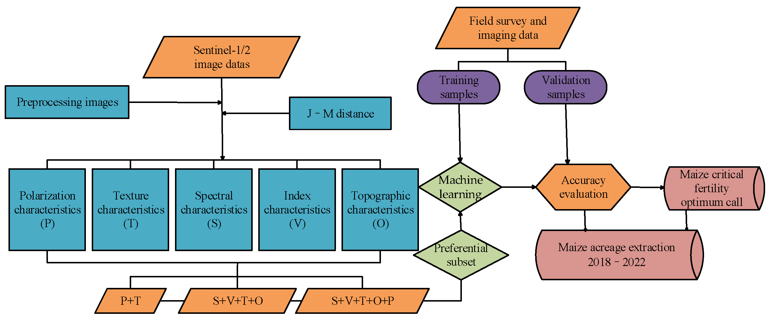
The Sentinel-1 SAR GRD data collected for this study throughout each maize growth cycle were polarized in the Interferometric Wide (IW)-Swath mode in both VH and VV modes. These data underwent preprocessing, which included orbital corrections, topographic adjustments, radiometric calibration, and thermal noise removal. Sentinel-2 is a high-resolution multispectral imaging satellite that uniquely features 3 red-edge bands and covers 13 spectral bands, ranging from visible and near-infrared to short-wave infrared. To categorize the target images, we employed the Sentinel-2 Level-2A product, specifically selecting images with less than 20% cloud cover. The QA60 band was utilized to mask and remove cloud information from the images. We stacked and cropped the selected spectral bands with spatial resolutions of 10 m and 20 m for further analysis.

3. Research Methods

This study aims to investigate remote sensing identification methods in order to accurately determine the planted area of maize during its crucial fertility phase. The technological approach is illustrated in Figure 2. First, the J–M distance method is used to compare the separability of maize from other covers in various phenological periods. Next, the random forest algorithm is used to construct a crop classification model based on the optimal features of Sentinel-1 and Sentinel-2 data. The accuracy of maize recognition in each fertility period and the impact of various feature sets on the accuracy of maize extraction are compared. Finally, the maize planting areas from 2018 to 2022 are extracted using the optimal feature classification approach, and the spatial distribution characteristics of the planting structure are quantitatively analyzed.

3.1. Characteristic Variable

Table 2. Characteristic variable.

Sensors	Group	Characteristic Variable
Sentinel-1	Polarization features	VV
		VH
		VV + VH, VV − VH, VV × VH, VV/VH
Sentinel-2	Spectral features	Blue, green, and red bands (B2, B3, B4)
		Red band (B5, B6, B7)
		Near-infrared band (B8, B8A)
		Short infrared band (B11, B12)
	Exponential features	Normalized Difference Vegetation Index (NDVI)
		Bare Soil Index (BSI)
		Plant Senescence Reflectance Index (PSRI)
		Red-edge Position Index (REPI)
		Normalized Difference Water Index (NDWI)
		Enhanced Vegetation Index (EVI)
		Normalized Difference Building Index (NDBI)
		Green Chlorophyll Vegetation Index (GCVI)
	Topographic features	Elevation
		Aspect
		Shadow
		Slope
Sentinel-1/2	Texture features	Contrast
		Correlation
		Variance
		Inverse Difference Moment (IDM)
		Entropy
		Angular Second Moment (ASM)

displays the selection of characteristic variables, which include polarization, texture, and spectral features in Sentinel-1 data and spectral, index, and topographic features in Sentinel-2 data. Sentinel-1′s polarization features are constructed using VV, VH, and related operations, as they are not affected by clouds or fog, making it possible to gather key feature properties. Texture features are crucial for gathering crop information from images. The chosen features include entropy, contrast, correlation, variance, inverse moments, and the commonly utilized angular second-order moments. Spectral features are constructed by selecting the original Sentinel-2 bands across different growth periods. Index attributes, such as NDVI [25], BSI [26], PRSI [27,28], NDWI [29], NDBI [30], and GCVI [31], are calculated based on the spectral reflectance of the actual maize. Using the reflectance of the Sentinel-2 red-edge region to calculate the vegetation index can improve the classification accuracy [32], so the REP is constructed by utilizing its red-edge band [33,34].

3.2. Classification Methods

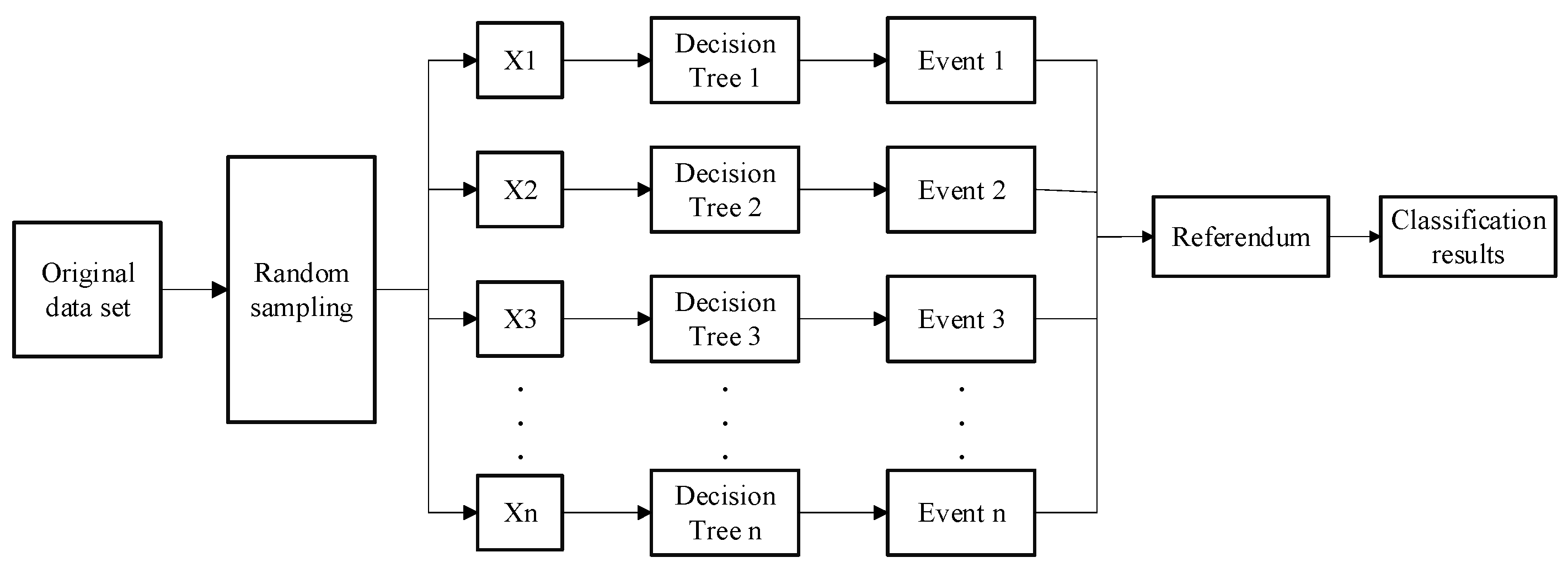
3.2.1. Random Forest Algorithm

The RF classification algorithm operates on the principle of aggregating weak classifiers to form a strong classifier. This method offers strong noise immunity, little human influence, enhanced classification capacity, and effective handling of diverse datasets [35,36]. The process involves using bootstrap resampling to randomly select training and test samples, which are then input into each classification tree to form a random forest. Finally, the results from multiple weak classifiers are combined through a voting mechanism to form a strong classifier for classification and prediction [37,38]. Random forests are widely used in the crop classification of remote sensing satellite images due to their ability to evaluate feature importance and handle high-dimensional data more effectively than other methods [39,40]. The overall process of this method is shown in Figure 3. In this study, the random forest classification algorithm was used to extract the maize growing area in the study area after combining the generated feature variables with the sample data from independent spectral bands. The parameters were adjusted to optimize both extraction accuracy and computational efficiency. The sampling ratio was set to 0.8, and the number of decision trees was fixed at 200, following the observed trend of accuracy improvement with an increasing number of trees.

3.2.2. Support Vector Machine (SVM) Algorithm

The SVM is a supervised learning algorithm extensively used for both classification and regression tasks. Its primary objective is to identify the optimal hyperplane that effectively separates samples from different classes while maximizing the margin between them, thereby minimizing classification errors. SVMs employ kernel functions to address nonlinear problems by mapping samples into a high-dimensional feature space. This approach enables SVMs to manage high-dimensional data and complex decision boundaries efficiently, making them particularly well suited for datasets with small sample sizes while maintaining robust performance.

3.2.3. Decision Tree (DT) Algorithm

The DT is a classification method used in decision analyses, characterized by its tree-like structure. The core principle involves categorizing samples into different classes through a series of decision nodes, which are essentially questions based on the characteristics of the data. Constructing a decision tree involves identifying the optimal attributes for splitting the data. In this process, the concepts of entropy and information entropy are pivotal. Entropy measures the uncertainty or disorder within a dataset, while information entropy quantifies the uncertainty of the data with respect to a specific attribute. By evaluating the change in information entropy before and after a split, the decision tree selects the attribute that minimizes uncertainty, thereby guiding the optimal division of the dataset.

3.2.4. Naive Bayes (NB) Algorithm

The NB algorithm is a classification method grounded in Bayes’ theorem and assumes conditional independence among features. The core principle involves applying Bayes’ theorem to calculate the posterior probability of each class for a given data sample, then selecting the class with the highest posterior probability as the predicted category. The algorithm assumes that features are independent of one another, which simplifies computations but can impact classification accuracy. Despite this assumption, Naive Bayes is valued for its simplicity and efficiency in learning, making it a popular choice for various classification tasks.

3.2.5. K-Nearest Neighbor (KNN) Algorithm

The KNN algorithm classifies a sample by first computing the distance between it and every sample in the training set. It then selects the K samples with the smallest distances, referred to as “neighbors”. Finally, the algorithm determines the category of the sample to be classified by either voting among the neighbors’ category labels or using a weighted average.

3.3. Separability Calculations

The J–M distance technique is a way to categorize multispectral remote sensing images. It accounts for the influence between different categories and is effective in managing significant disparities in class separability. It can be used to measure the separability between different feature classes [41,42]. The formula for the J–M distance is shown below:

$$JM=2\left(1-e^{{-B}_{ij}}\right)$$

(1)

$$B_{ij}={\displaystyle \frac{1}{8}}\left(m_i-m_j\right){\displaystyle \frac{2}{{{\sigma }_i}^2+{{\sigma }_j}^2}}+{\displaystyle \frac{1}{2}}\ln \left({\displaystyle \frac{{{\sigma }_i}^2+{{\sigma }_j}^2}{2{\sigma }_i{\sigma }_j}}\right)$$

(2)

where $B_{ij}$ represents the Bhattacharyya distance, JM is the J–M distance between categories i and j; $m_i$ and $m_j$ are the means of the feature vectors corresponding to the samples; ${\sigma }_i$ and ${\sigma }_j$ are the standard deviations of the feature vectors corresponding to the samples.

3.4. Feature Preferences

Previous studies have shown that classifier performance may decline when an excessive number of feature variables is introduced [43,44]. Feature selection and optimization are critical in remote sensing image classification to address issues such as overfitting caused by too many variables and poor classification performance due to computational complexity. The random forest algorithm inherently leverages out-of-bag (OOB) data and employs an internal function to rank feature importance. By selecting the highest-ranked features, it achieves optimal classification performance.

3.5. Precision Evaluation

The confusion matrix is a standard method for evaluating the accuracy of remote sensing image classification results [45]. In this study, we use the errorMatrix function to calculate the confusion matrix. To comprehensively evaluate the remote sensing recognition of maize using different machine learning classification methods, we consider four evaluation metrics: user accuracy (UA), producer accuracy (PA), overall accuracy (OA), and the Kappa coefficient [46].

4. Results and Discussion

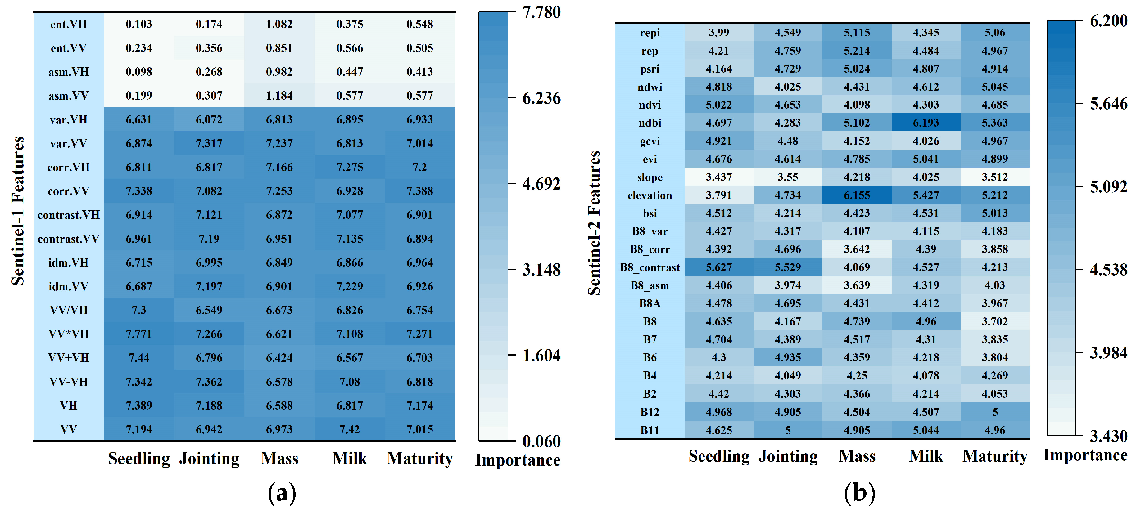
4.1. Analysis of Feature Selection

We incorporated features such as the spectral reflectance of maize from 2022 remote sensing images of the study area. A total of 36 feature variables were included in the multi-source dataset, which were then fed into the RF classifier. The features were ranked in descending order of importance, and the experiment was repeated until the classification accuracy reached a stable point, with no significant further increases or decreases.

As shown in Figure 4, the relationship between the number of classification features and classification accuracy reveals an initial rise, followed by a decline, and then a gradual stabilization as the number of features increases. The classification accuracy stabilizes when the number of features fluctuates between 9 and 25. As the number of features increases from 4 to 9, classification accuracy improves from 0.65 to 0.91; however, once the number of features exceeds 28, the classification accuracy no longer consistently increases but rather fluctuates. The highest classification accuracy of 0.93 is achieved with 28 features. Beyond this, the accuracy plateaus, stabilizing around 0.90. Given that an increase in the number of features impacts computational efficiency, we selected the top 28 most significant features for our analysis. These included eight raw spectral features (B2; B4; B6; B7; B8; B8A; B11; and B12), nine spectral indices (B2; B4; B6; B7; B8; B8A; B11; and B12), six polarization features (VV; VH; VV_VH_ratio; VV_minus_VH; VV_plus_VH; and VV_times_VH), four texture elements (B8_contrast; B8_corr; B8_var; and B8_asm), and one terrain feature (elevation).

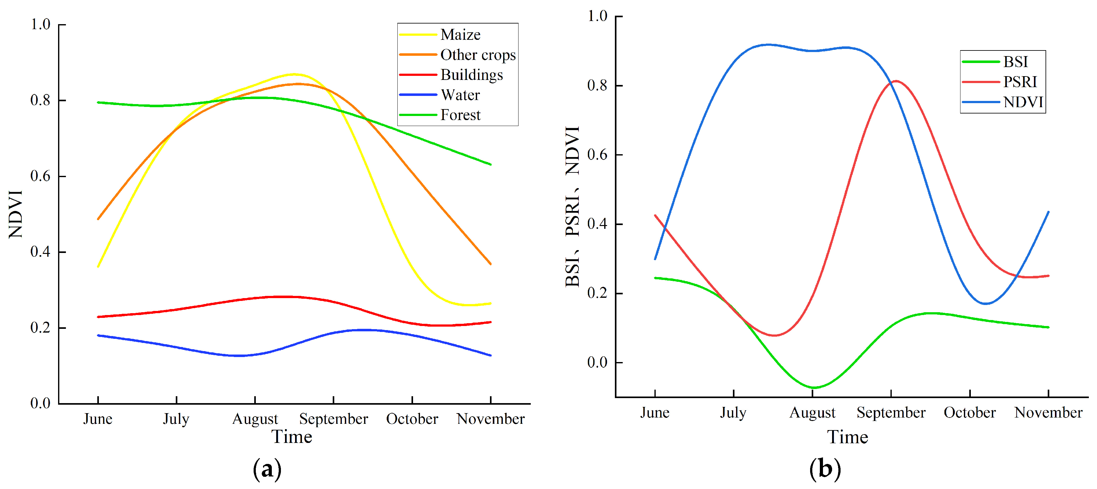
4.2. Analysis of Critical Time Phases

Due to variations in growth cycles, different features exhibit distinct vegetation index characteristics during the same time period. In this study, we utilized sample point data to generate NDVI curves for various features throughout the maize growth period, as illustrated in Figure 5a. Additionally, we plotted NDVI, BSI, and PSRI curves for maize in different time periods, as shown in Figure 5b. The equations used to calculate the NDVI, BSI, and PSRI are as follows:

$$NDVI={\displaystyle \frac{B_8-B_4}{B_8+B_4}}$$

(3)

$$BSI={\displaystyle \frac{B_{11}+B_4-\left(B_8+B_2\right)}{B_{11}+B_4+B_8+B_2}}$$

(4)

$$PSRI={\displaystyle \frac{B_4-B_2}{B_6}}$$

(5)

where $B_2$, $B_4$, $B_6$, $B_8$, and $B_{11}$ represent the 2, 4, 6, 8, and 11 bands of Sentinel-2, respectively.

Figure 5 shows that the NDVI values of buildings, water bodies, and woodlands remained relatively stable from June to November. In contrast, summer crops, including maize, gradually matured between July and August, with their NDVI values peaking in mid-August before gradually declining to their lowest levels from mid-August to October as the crops, including maize, reached full maturity and were harvested. Additionally, the NDVI, BSI, and PSRI curves for corn exhibited clear patterns. During the tasseling stage, the BSI and PSRI values were at their lowest, while the NDVI value was at its highest. This is because maize is in a good state of growth during this period, with a relatively high chlorophyll content, good growth, and the strongest absorption of red light and reflection of near-infrared light.

4.3. Separability Results for Different Land Use Types

The results of the separability of maize from other features in different growth periods are shown in

Table 3. J–M distance between maize and other features.

Type of Training Samples	Seedling Stage	Jointing Stage	Tasseling Stage	Milk Stage	Ripening Stage
Other crops	1.81	1.92	1.98	1.77	1.83
Building	1.99	1.99	1.99	1.98	1.97
Water	1.99	1.99	1.99	1.99	1.99
Forest	1.97	1.99	1.99	1.99	1.98

. Separability from buildings, water bodies, and woodlands was high, but separability from other crops was poor, with the lowest value of 1.77 at the milk stage and the highest of 1.98 at the tasseling stage. During the tasseling stage, the separability of maize from buildings, water bodies, and woodlands was 1.99. For maize, separability from other crops was strongest during the tasseling stage, and it remained highly distinct from other features throughout the reproductive phase. The closer the J–M distance is to 2, the higher the separability between the two classes, and vice versa.

4.4. Categorization Results

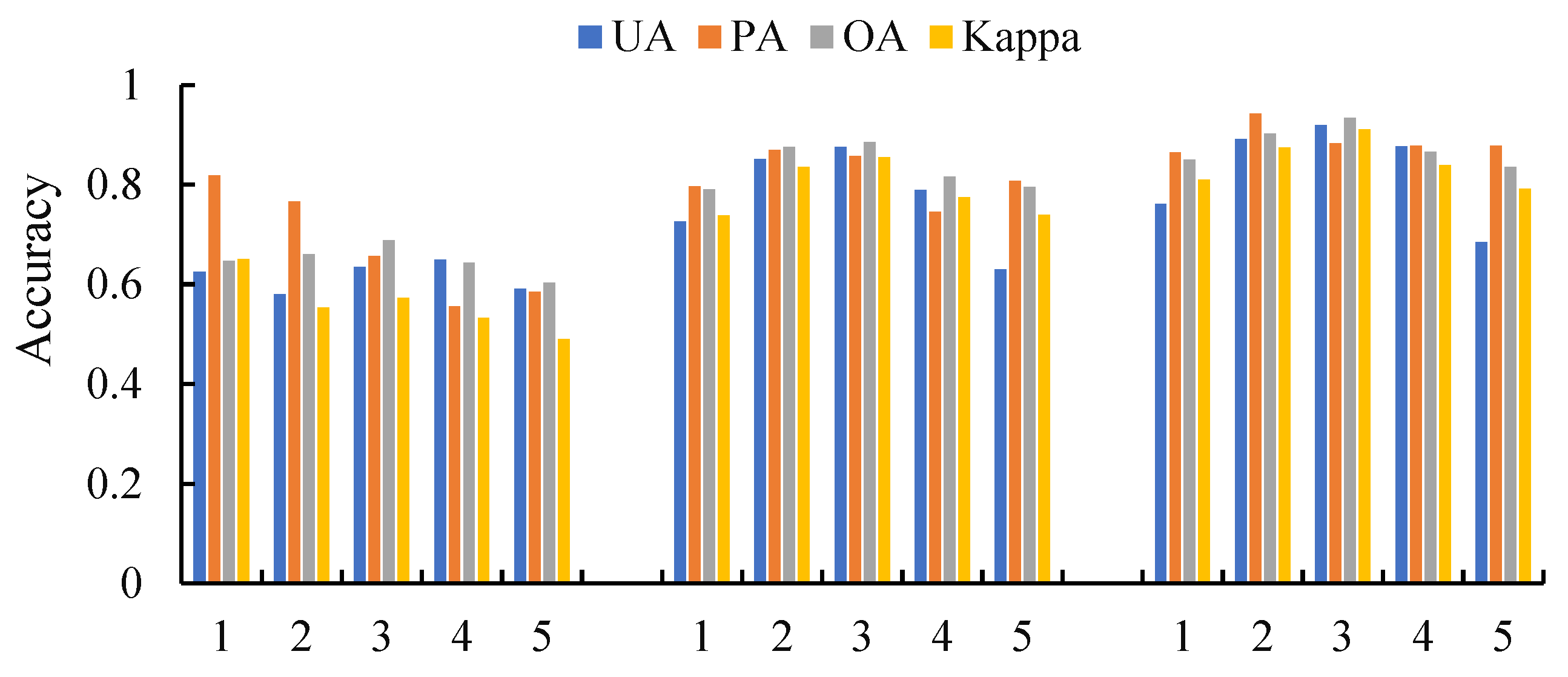
4.4.1. Classification of Single-Source Data

The median values of the image data were synthesized using Sentinel-1 and Sentinel-2 datasets from five distinct growth periods contained. Each period contained 18 feature variables for the Sentinel-1 images and 23 feature variables for the Sentinel-2 images. To minimize computation while maintaining a high classification accuracy, in this study, an RF classification model was constructed based on the GEE.

Table 4. Single-source Sentinel maize growth stage classification accuracy.

Classifications	Sentinel-1				Sentinel-2
	UA/%	PA/%	OA/%	Kappa	UA/%	PA/%	OA/%	Kappa
Seedling stage	72.62	81.85	64.70	0.65	72.62	79.64	79.02	0.74
Jointing stage	58.03	76.56	66.01	0.55	85.07	86.96	87.51	0.83
Tasseling stage	63.48	65.65	68.78	0.57	87.50	85.71	88.52	0.86
Milk stage	64.85	55.53	64.25	0.53	78.84	74.54	81.55	0.77
Ripening stage	89.04	58.44	60.33	0.49	63.01	80.71	79.53	0.74
All stages	62.29	56.32	58.20	0.46	64.91	78.43	75.85	0.68

displays the accuracy of the single-source model test set. The relative importance of each feature was calculated using the ee.Dictionary.map function, as shown in Figure 6.

The results indicate that the classification accuracy based on Sentinel-1 and Sentinel-2 data across all phenological stages was lower than that of single-stage classification, with overall accuracies (OAs) of 58.2% and 75.85%, respectively, which are insufficient to meet the classification requirements. The overall accuracy of classification across the five single phenological stages of Sentinel-1 was notably low. The highest accuracy was observed at the tasseling stage (68.78%, Kappa = 0.57), followed by the nodulation, milk, and seedling stages. The lowest accuracy was observed at the maturity stage (60.33%, Kappa = 0.49). Figure 6 shows that across all five fertility stages, the weights of entropy and the inverse difference moment were significantly smaller than those of the other features; the weights of several other polarization features and texture features were all in the range of 6 to 8 and did not differ significantly from one another. The overall classification performance was weak and strongly influenced by the phenological stage.

The overall classification accuracy of the Sentinel-2 data exceeded 79% for all individual reproductive stages, except for the full reproductive stage. The highest accuracy was observed at the spike stage (88.52%, Kappa = 0.86), followed by the scion stage (87.51%, Kappa = 0.83), the milk stage (81.55%, Kappa = 0.77), and the maturity stage (79.53%, Kappa = 0.74). The lowest accuracy occurred during the seedling stage (79.02%, Kappa = 0.74). The slope feature consistently had minimal influence throughout the stages, while other feature weights showed little variation. However, the elevation feature during the tasseling stage and the NDBI feature during the milk stage were notably prominent. Overall, classification accuracy increased from the seedling stage to the tasseling stage, where it peaked, before declining during the ripening stage. The classification performance of the single-source Sentinel-2 data was significantly superior to that of Sentinel-1 data, particularly in terms of accuracy.

4.4.2. Classification of Multi-Source Data Fusion

The features of Sentinel-1 and Sentinel-2 were independently fused based on the five growth stages of maize and the complete reproductive period. After feature selection, each period utilized the 28 selected feature variables mentioned above. All synthetic images were resampled to a spatial resolution of 10 m, and the RF method was then applied for classification. The classification accuracy results are shown in

Table 5. Classification accuracy for each growth period of multi-source.

Classifications	Seedling Stage		Jointing Stage		Tasseling Stage		Milk Stage		Ripening Stage		All Stages
	UA/%	PA/%	UA/%	PA/%	UA/%	PA/%	UA/%	PA/%	UA/%	PA/%	UA/%	PA/%
Maize	76.11	86.44	89.09	94.23	91.90	88.23	87.71	87.77	68.49	87.72	56.45	62.50
Other crops	76.92	66.66	88.13	85.24	90.65	85.24	82.00	86.10	79.16	61.29	71.64	66.66
Building	93.87	95.83	88.67	95.91	92.52	96.42	87.72	83.22	90.01	91.84	93.33	98.24
Water	100	100	90.90	100	92.00	100	96.97	96.30	95.98	96.16	97.65	94.16
Forest	88.09	86.04	95.55	82.69	93.22	91.85	86.47	86.33	93.22	90.16	82.05	75.92
OA/%	85.00		90.17		93.38		86.51		83.53		76.77
Kappa	0.81		0.87		0.91		0.84		0.79		0.69

. The lowest overall classification accuracy of 76.77% was achieved for the complete fertility period. The highest overall accuracy was achieved during the tasseling stage, reaching 93.38% with a Kappa coefficient of 0.91. This was followed by the jointing stage with 90.17% accuracy and a Kappa coefficient of 0.87; the milk stage, with 86.51% accuracy and a Kappa coefficient of 0.84; and the seedling stage, with 85.00% accuracy and a Kappa coefficient of 0.81. The accuracy at maturity was the lowest among the five reproductive stages, being 83.53% with a Kappa coefficient of 0.79. Classification accuracy for buildings and water bodies remained high across all stages. Forest classification was less affected by time, while maize and other crops were more influenced by phenological stages. The overall accuracy increased from the seedling stage to the maturity stage before decreasing. Overall, multi-source remote sensing images provided higher classification accuracies than single-source Sentinel-1/Sentinel-2 data, with the best performance observed during the tasseling stage throughout the entire growth cycle.

We used the SVM, DT, NB, and KNN methods on the GEE to identify the features of maize at the tasseling stage in Jiaozuo City in 2022, in addition to the RF classification method, in order to investigate the classification accuracy of multi-source data fusion with various machine learning methods. Next, in order to increase the decision-making process’s dependability, a bootstrapping simulation was run to evaluate the remote sensing classification model’s prediction confidence. By repeatedly conducting random sampling, the simulation technique creates several training and test sets, from which a classification model’s confidence ranges and error estimates are derived. The mean accuracy represents the model’s average classification accuracy over all simulations, whereas the standard deviation of performance indicates how much the model’s performance varies throughout simulations. The classification results for each method are summarized in

Table 6. Maize classification accuracy of different machine learning classification methods at tasseling stage.

Classification Methods	RF	SVM	DT	NB	KNN
OA	93.38	91.76	90.94	82.72	91.18
Kappa	0.91	0.89	0.88	0.78	0.89
Mean Accuracy	0.902	0.870	0.871	0.786	0.891
Standard Deviation of Accuracy	0.014	0.037	0.021	0.027	0.019

. Among the methods, RF has the highest mean accuracy, Kappa value, and overall accuracy (93.38%, 0.91, and 0.902, respectively). The fact that RF has the lowest accuracy standard deviation means that under various configurations for the training and test sets, its accuracy fluctuates very little—roughly 1.4%. With respect to the OA, Kappa value, and mean accuracy, NB has the lowest values (82.72%, 0.78, and 0.786, respectively). The SVM has the largest shift in accuracy. The outcomes demonstrate that the RF model outperforms the other four models and operates more steadily, with minimal variation in the forecast results.

Figure 7 shows the accuracy distribution of the five models over multiple simulations. The x-axis indicates the number of iterations of the simulation (i.e., different combinations of training and test sets), and the y-axis indicates the classification accuracy in each iteration. The data points in the figure show the accuracy variations of the models in different simulations. In the figure, it can be seen that both the RF and KNN data points are more densely distributed, and the variation of RF is smaller than that of KNN, which indicates that the model is more stable and has less error. In contrast, the NB, DT, and SVM data points fluctuate more, indicating that the model performs unstably under different training–testing splits, and there is greater uncertainty. Overall, the RF classification is the best, but there is still room for improvement.

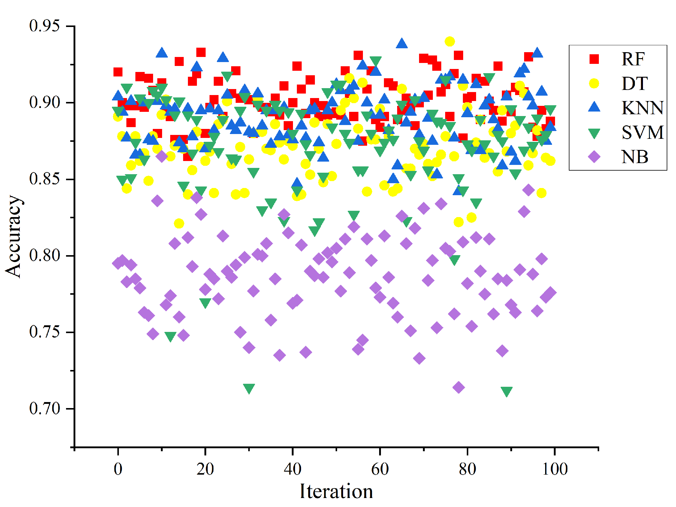
4.5. Comparative Analysis of Classification Accuracy

A comparative analysis of the recognition accuracy of maize at different growth stages in terms of single-source datasets and multi-source fusion datasets is illustrated in Figure 8. The classification accuracies at the tasseling stage are 68.78%, 88.52%, and 93.38% for the three methods, with Kappa coefficients of 0.57, 0.86, and 0.91, respectively. Stages 1 to 5 correspond to the seedling, jointing, tasseling, milk, and ripening stages of maize, respectively. The overall classification accuracy of the tasseling stage of maize is the highest among the three methods, reaching 68.78%, 88.52%, and 93.38%, with Kappa coefficients of 0.57, 0.86, and 0.91, respectively. The jointing stage also shows a relatively high accuracy and good recognition results. In contrast, the seedling and ripening stages are less effective due to the vigorous growth of maize during the jointing-tasseling period, which creates a clear contrast with other surface features. However, during the milk and ripening stages, maize grows slowly and becomes less distinguishable from other surface features, leading to a reduced recognition accuracy. Among the three approaches, the fused active–passive remote sensing images achieve the highest accuracy, while the single-source Sentinel-1 images have the lowest accuracy. At the jointing stage, the single-source Sentinel-2 images show a 2.66% increase in overall classification accuracy and a 0.04 increase in the Kappa coefficient compared with the Sentinel-1 images. The fused Sentinel images demonstrate a 24.16% increase in overall classification accuracy and a 0.32 increase in the Kappa coefficient relative to single-source Sentinel-1 images. In comparison with the single-source Sentinel-1 images, the fused active–passive remote sensing images increase the overall classification accuracy by 24.6% and the Kappa coefficient by 0.34 during the tasseling period and by 4.86% and 0.05 during the milk stage, respectively. The increase in accuracy at the jointing stage is 2.66% with a Kappa coefficient improvement of 0.04. Figure 9 illustrates three areas with significant classification discrepancies within the study area. Each row represents a discrete geographical area, while the columns show the synthesized true-color and false-color images, single-source Sentinel-1 and -2 classification maps, and the fused Sentinel-1 and -2 classification maps for each area at the tasseling stage. These results show that maize exhibits a dark green hue on the true-color image and a dark red hue on the false-color image. The fused Sentinel classification outperforms the single-source Sentinel classifications by providing a more accurate and complete extraction of maize planting areas.

The distribution map of maize plantings extracted from the fused Sentinel-1 and Sentinel-2 images during the tasseling period was used as a reference for a comparison with the maize extraction distribution maps of the other four periods in 2022. The resulting difference map shown in Figure 10 illustrates the variation in maize area across the different growth periods in comparison with the tasseling period. Green denotes TP (true positive, i.e., maize identified in both periods), red represents FP (false positive; i.e., non-maize in the tasseling period but maize in the other periods), and blue denotes FN (false negative, i.e., identified as maize in the tasseling period but not in the other periods). The proportions of the TP, FP, and FN pixels relative to the predicted and actual maize pixels are denoted by a, b, and c, respectively. A higher proportion of a indicates greater similarity in maize recognition between the two periods, while larger proportions of b and c indicate greater differences. The proportion of a is the highest at 83.5% during the jointing stage, with relatively small proportions of b and c at 4.5% and 12%, respectively, indicating the smallest difference in maize identification from the tasseling stage. Conversely, at the seedling stage, the proportion of a is 81%, which is relatively lower, while the proportions of b and c are 8.5% and 10.5%, showing the largest difference in maize identification from the tasseling stage.

Five representative maize planting regions (a–e) were selected to further analyze maize recognition differences. The maize classification results for these regions are shown in Figure 11, where 1–5 represent the seedling, jointing, tasseling, milk, and ripening stages. The tasseling stage shows the best recognition performance, with superior accuracy in areas of flat terrain and dense planting. However, in relatively fragmented and complex areas, classification errors are higher during the other periods than during the jointing and tasseling stages, especially during the seedling stage as shown in area a. The classification accuracy during the seedling stage is notably inadequate. Thus, in remote sensing image classification research, topography also plays a significant role in determining the accuracy of maize identification using the RF classification. The accuracy of recognition decreases with an increasing land use fragmentation and complex topography.

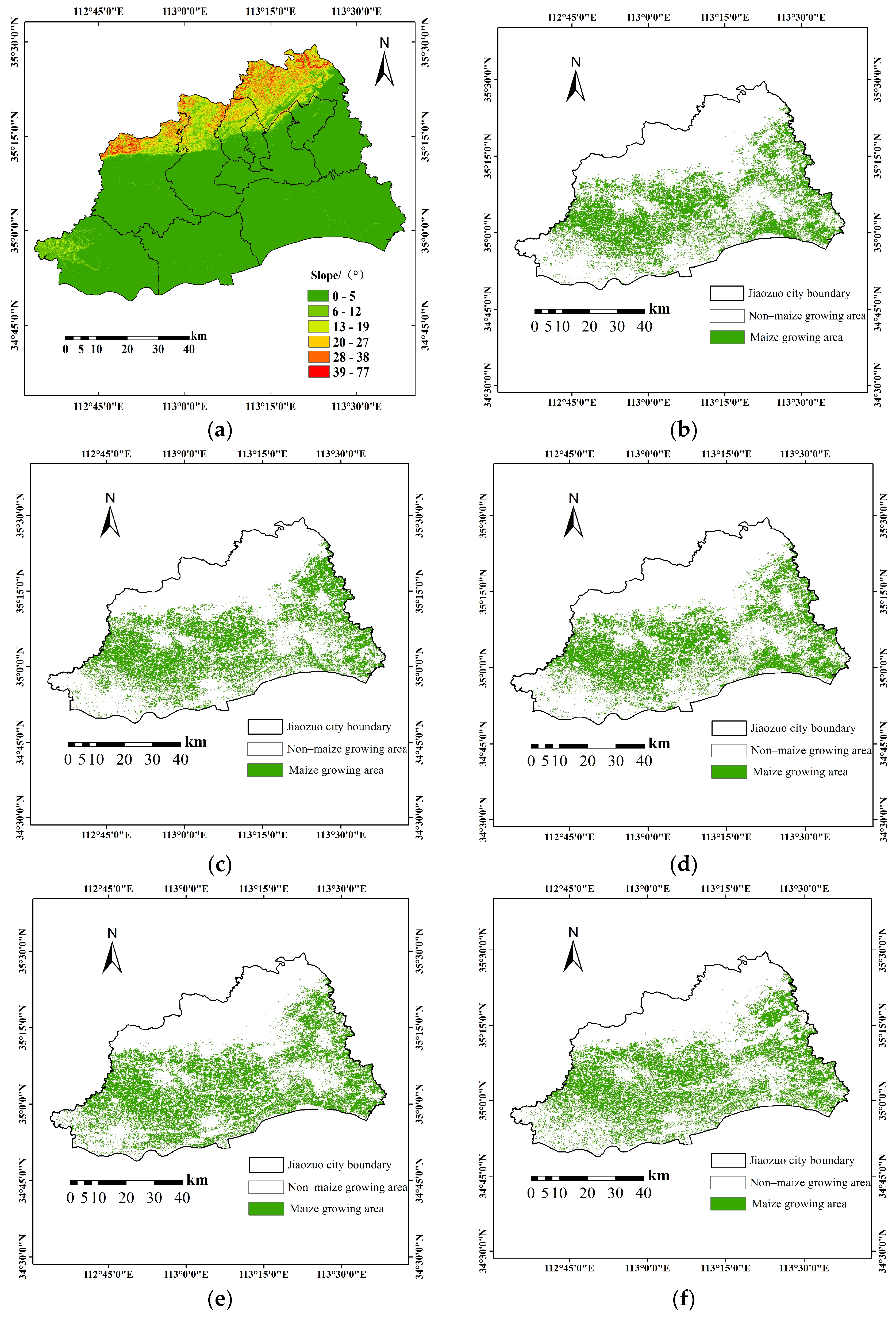
4.6. Results of Maize Area Extraction and Accuracy Confirmation

Figure 12 displays the results of extracting the maize planted area in Jiaozuo City from 2018 to 2022 based on the tasseling stage. The highest accuracy of maize area extraction was achieved by fusing the active and passive remote sensing feature sets during the tasseling period. The sum of the maize areas in each pixel within the study region represents the total area of maize. The ratio of the extracted area to the ground truth value, which was derived from the Henan Provincial Statistical Yearbook, indicates the accuracy of the results for the maize sown area. The accuracy was calculated using the following formula [47]:

$$P=1-{\displaystyle \frac{\left|S-S^1\right|}{S^1}}\times 100\%$$

(6)

where $S$ is the sown area retrieved using the technique employed in this study, $P$ is the precision of the extracted area, and $S^1$ is the actual planted area of maize.

DEM data were used to generate a slope distribution map of Jiaozuo City, as shown in Figure 12a. This map illustrates the wide range of maize planting, which is associated with slope: the steeper the terrain, the smaller the area of maize distribution, as in the northern region; additionally, there is a significant increase in maize planting in the southwestern direction of Jiaozuo City, particularly in Mengzhou.

Table 7. Comparison of remote sensing-extracted sown area and statistical sown area of maize in Jiaozuo City.

Year	Extracted Area (hm2)	Statistical Area (hm2)	Absolute Error (hm2)	Accuracy (%)	OA (%)	Kappa
2018	113,708	121,190	7482	93.83	91.45	0.89
2019	117,944	119,410	1466	98.77	94.97	0.93
2020	120,809	123,400	2591	97.90	91.81	0.89
2021	122,596	126,390	3794	97.00	94.72	0.93
2022	124,490	126,960	2470	98.06	93.38	0.91

displays the precision and accuracy of maize area extraction based on the tasseling period. In 2019, the accuracy was the highest at 98.77%, with the overall accuracy of the classification being 94.97%, with a Kappa coefficient of 0.93. This was followed by 2022, 2020, and 2021. The year 2018 had the lowest accuracy at 93.83%, with the overall accuracy of the classification being 91.45%, with a Kappa coefficient of 0.89. The period from 2019 to 2022 showed a growth trend in maize planting, with only a slight increase, consistent with the change in the corn sowing area in the Henan Provincial Bureau of Statistics.

4.7. Discussion

The potential for using active–passive remote sensing data during critical reproductive periods in urban land use classification studies is significant [48]. Ensuring food security requires careful observation of the maize planted area. For the purposes of tracking maize growth and estimating crop yield, it is highly advantageous to determine the planted area of maize before its maturity. In this study, maize in the study area could be quickly and accurately identified, and a map of the maize planted area in the previous five years was precisely created from remote sensing images taken during the tasseling stage. This information is useful for managing and tracking the growth of maize approximately 4–6 weeks prior to harvest [49]. It is beneficial for the agricultural sector to predict the total maize production accordingly [50]. In addition to being able to identify crops such as oilseed rape and winter wheat rapeseed, combining Sentinel-1 and Sentinel-2 images improves the accuracy of maize identification compared with using only one set of data [51,52]. This is particularly important for research conducted in areas that are prone to summertime cloud cover and precipitation. The combined active–passive remote sensing classification can be expanded to include other urban regions that are known for having smog, clouds, haze, and a high surface soil moisture content. However, there are still limitations to the methodology of this study. The RF model is highly dependent on samples for training. RF requires manual feature selection and the pre-definition of the crop growth stage, whereas deep learning can overcome this problem and generate high-dimensional features [53,54,55]. For example, Wang et al. developed a Deep Adaptation Crop Classification Network (DACCN) [56,57]. With total classification accuracies ranging from 0.835 to 0.92, they discovered that the DACCN performed better than other models (RF and SVM). A possible advancement in the future is the use of deep neural networks for early crop mapping. The distribution of maize was determined in this study using a sizable dataset that was retrieved from the GEE cloud platform. In terms of practicality, this strategy is useful. Future monitoring and yield-estimating initiatives aiming to enhance the efficacy of sustainable development can utilize this work as a starting point.

4.8. Uncertainty and Outlook

We discussed and analyzed the extraction of maize planting areas using remote sensing data from five distinct fertility stages and compared the results across various machine learning methods. While the outcomes were generally promising, certain limitations persist. Several key issues require further exploration to enhance the accuracy and robustness of the findings.

• This study utilized Sentinel-1 and Sentinel-2 images with a spatial resolution of 10 m, which may have introduced limitations due to the potential presence of mixed land cover types within individual pixels, thus affecting classification accuracy. Furthermore, the northern part of the study area is characterized by a complex mountainous terrain, which could also have influenced the results. Future research should incorporate high-resolution images to produce more detailed datasets and investigate their impact on classification performance.
• The machine learning methods and feature variables employed in this study are tailored to a specific study area, and their generalizability to other regions or larger areas remains uncertain, warranting further investigation. Future research should evaluate the applicability of these models and variables in diverse geographical contexts. Additionally, deep learning models, which have shown promise in remote sensing applications, could be explored as alternative approaches for the extraction of maize planting areas.
• To further enhance the extraction of maize areas from multi-source data, future research should focus on capturing the developmental characteristics of maize across different growth stages. By continuously optimizing the selection of feature types from Sentinel-1 and Sentinel-2 for each phenological phase, the classification process could more precisely reflect changes at each stage. This refined feature selection is expected to improve classification accuracy and strengthen the overall performance of maize area detection.
• The quality of the remote sensing images collected during different maize growth stages can vary, potentially influencing the results. Satellites are subject to both internal and external factors when capturing ground images, with meteorological conditions being a major influence. Although efforts are made to screen for cloud cover, the impact of weather conditions on the accurate recognition of maize remains a concern and cannot be entirely eliminated.

5. Conclusions

This study focused on maize in Jiaozuo City, Henan Province. The separability of maize from other cover types at different fertility stages was calculated using Sentinel-1 and Sentinel-2 images as the main data source. Features such as polarization, texture, and the vegetation index were constructed to facilitate this process. A machine learning algorithm was employed to ascertain the distribution of maize at different fertility stages. The main conclusions are as follows:

1.

The classification accuracy of fused active–passive remote sensing images for the 2022 maize tasseling period improved by 24.6% relative to that of the single-source Sentinel-1 images, with the Kappa coefficient increasing by 0.34. Compared with the single-source Sentinel-2 images, the accuracy improved by 4.86% and the Kappa coefficient increased by 0.05. Thus, using multi-source data with the random forest algorithm provided a higher accuracy and better classification of maize than using the Sentinel-1 or Sentinel-2 images. Based on multi-source data, RF had a higher classification accuracy in the tasseling stage than the SVM, DT, NB, and KNN methods.

2.

During the tasseling period, the general accuracy of the extracted maize planted area was at its maximum. The multi-source data fusion random forest classification in 2022 had an overall accuracy of over 85% and Kappa coefficients over 0.79. Among these, the tasseling stage had the highest overall accuracy at 93.38% and a Kappa coefficient of 0.91, indicating that this method can help the agricultural insurance department assess risks promptly and verify the planted area quickly.

3.

This study used the random forest method to extract the maize area in Jiaozuo City from 2018 to 2022. The extracted accuracies were 93.83%, 98.77%, 97.9%, 97%, and 98.06%, respectively. The remotely extracted maize planted area in Jiaozuo City showed a growing trend in 2019–2022, which is consistent with the Statistical Yearbook. The extracted data were combined with active–passive remote sensing fusion images taken during the tasseling stage. Furthermore, the random forest’s ability to identify features was influenced by the terrain factor. Specifically, steep slopes are less suitable for maize planting, while flatter areas support a larger maize planting range. Furthermore, the classification effect in flat terrain is superior to that in complex terrain.

References

1. Chen, Z.; Reng, J.; Tang, H.; Shi, Y.; Len, P.; Liu, J.; Wang, L.; Wu, W.; Yao, Y.; Hasiyuya. Progress and perspectives on agricultural remote sensing research and applications in China. J. Remote Sens. 2016, 20, 748–767. [Google Scholar] [CrossRef]
2. Meng, S.; Zhong, Y.; Luo, C.; Hu, X.; Wang, X.; Huang, S. Optimal Temporal Window Selection for Winter Wheat and Rapeseed Mapping with Sentinel-2 Images: A Case Study of Zhongxiang in China. Remote Sens. 2020, 12, 226. [Google Scholar] [CrossRef]
3. Zhang, F.; Zhang, J.; Duan, Y.; Yang, Z. Transferring Deep Convolutional Neural Network Models for Generalization Mapping of Autumn Crops. Natl. Remote Sens. Bull. 2024, 28, 661–676. [Google Scholar] [CrossRef]
4. Tang, H. Progress and Prospect of Agricultural Remote Sensing Research. J. Agric. 2018, 8, 175–179. [Google Scholar] [CrossRef]
5. Dong, J.; Wu, W.; Huang, J.; You, N.; He, Y.; Yan, H. State of the Art and Perspective of Agricultural Land Use Remote Sensing Information Extraction. J. Geo-Inf. Sci. 2020, 22, 772–783. [Google Scholar] [CrossRef]
6. Guo, J.; Zhu, l.; Jin, B. Crop Classification Method with Differential Characteristics Based on Multi-temporal PolSAR Images. Trans. Chin. Soc. Agric. Mach. 2018, 49, 192–198. [Google Scholar]
7. Chen, Q.; Cao, W.; Shang, J.; Liu, J.; Liu, X. Superpixel-Based Cropland Classification of SAR Image with Statistical Texture and Polarization Features. IEEE Geosci. Remote Sens. Lett. 2022, 19, 4503005. [Google Scholar] [CrossRef]
8. Useya, J.; Shengbo, C. Exploring the Potential of Mapping Cropping Patterns on Smallholder Scale Croplands Using Sentinel-1 SAR Data. Chin. Geogr. Sci. 2019, 20, 626–639. [Google Scholar] [CrossRef]
9. Liao, C.; Wang, J.; Huang, X.; Shang, J. Contribution of Minimum Noise Fraction Transformation of Multi-Temporal RADARSAT-2 Polarimetric SAR Data to Cropland Classification. Can. J. Remote Sens. 2018, 44, 215–231. [Google Scholar] [CrossRef]
10. PAN, Z.; HU, Y.; WANG, G. Detection of Short-Term Urban Land Use Changes by Combining SAR Time Series Images and Spectral Angle Mapping. Front. Earth Sci. 2019, 13, 495–509. [Google Scholar] [CrossRef]
11. Liang, J.; Liu, D. A Local Thresholding Approach to Flood Water Delineation Using Sentinel-1 SAR Imagery. ISPRS J. Photogramm. Remote Sens. 2020, 159, 53–62. [Google Scholar] [CrossRef]
12. Markert, K.N.; Chishtie, F.; Anderson, E.R.; Saah, D.; Griffin, R.E. On the Merging of Optical and SAR Satellite Imagery for Surface Water Mapping Applications. Results Phys. 2018, 9, 275–277. [Google Scholar] [CrossRef]
13. Xie, Y.; Zhang, Y.; Xun, L. Crop Classification Based on Multi-source Remote Sensing Data Fusion and LSTM Algorithm. Chin. Soc. Agric. Eng. 2019, 35, 129–137. [Google Scholar] [CrossRef]
14. Li, C.; Chen, W.; Wang, Y.; Ma, C.; Wang, Y.; Li, Y. Extraction of Winter Wheat Planting Area in County Based on Multi-sensor Sentinel Data. Trans. Chin. Soc. Agric. Mach. 2021, 52, 207–215. [Google Scholar] [CrossRef]
15. Ma, Z.; Liu, C.; Xue, H.; Li, J.; Fang, X.; Zhou, J. Identification of Winter Wheat by Integrating Active and Passive Remote Sensing Data Based on Google Earth Engine Platform. Trans. Chin. Soc. Agric. Mach. 2021, 52, 195–205. [Google Scholar] [CrossRef]
16. Wu, X.; Hua, S.; Zhang, S.; Gu, L.; Ma, C.; Li, C. Extraction of Winter Wheat Distribution Information Based on Multi-phenological Feature Indices Derived from Sentinel-2 Date. Trans. Chin. Soc. Agric. Mach. 2023, 54, 207–216. [Google Scholar]
17. Liu, S.; Peng, D.; Zhang, B.; Chen, Z.; Yu, L.; Chen, J.; Pan, Y.; Zheng, S.; Hu, J.; Lou, Z.; et al. The Accuracy of Winter Wheat Identification at Different Growth Stages Using Remote Sensing. Remote Sens. 2022, 14, 893. [Google Scholar] [CrossRef]
18. Lv, W.; Song, X.; Yang, H. Extraction of Maize Acreage Based on Deep Learning and Multi-source Remote Sensing Data. Jiangsu Agric. Sci. 2023, 51, 171–178. [Google Scholar] [CrossRef]
19. Xie, Y.; Wang, J.; Liu, Y. Research on Winter Wheat Planting Area Identification Method Based on Sentinel-1/2 Data Feature Optimization. Trans. Chin. Soc. Agric. Mach. 2024, 55, 231–241. [Google Scholar] [CrossRef]
20. Qu, C.; Li, P.; Zhang, C. A Spectral Index for Winter Wheat Mapping Using Multi-Temporal Landsat NDVI Data of Key Growth Stages. ISPRS J. Photogramm. Remote Sens. 2021, 175, 431–447. [Google Scholar] [CrossRef]
21. Virnodkar, S.; Pachghare, V.K.; Patil, V.C.; Jha, S.K. Performance Evaluation of RF and SVM for Sugarcane Classification Using Sentinel-2 NDVI Time-Series. In Progress in Advanced Computing and Intelligent Engineering. Advances in Intelligent Systems and Computing; Panigrahi, C.R., Pati, B., Mohapatra, P., Buyya, R., Li, K.C., Eds.; Springer: Singapore, 2021; Volume 1199. [Google Scholar] [CrossRef]
22. Ponganan, N.; Horanont, T.; Artlert, K.; Nuallaong, P. Land Cover Classification Using Google Earth Engine’s Object-Oriented and Machine Learning Classifier. In Proceedings of the 2021 2nd International Conference on Big Data Analytics and Practices (IBDAP), Bangkok, Thailand, 26–27 August 2021; pp. 33–37. [Google Scholar] [CrossRef]
23. Zhou, R.; Yang, C.; Li, E.; Cai, X.; Yang, J.; Xia, Y. Object-Based Wetland Vegetation Classification Using Multi-Feature Selection of Unoccupied Aerial Vehicle RGB Imagery. Remote Sens. 2021, 13, 4910. [Google Scholar] [CrossRef]
24. Palchowdhuri, Y.; Valcarce-Diñeiro, R.; King, P.; Sanabria-Soto, M. Classification of multi-temporal spectral indices for crop type mapping: A case study in Coalville, UK. J. Agric. Sci. 2018, 156, 24–36. [Google Scholar] [CrossRef]
25. Tucker, C.J. Red and Photographic Infrared Linear Combinations for Monitoring Vegetation. Remote Sens. Environ. 1979, 8, 127–150. [Google Scholar] [CrossRef]
26. Huete, A.R. A Soil-Adjusted Vegetation Index (SAVI). Remote Sens. Environ. 1988, 25, 295–309. [Google Scholar] [CrossRef]
27. Tian, X.; Zhang, Y.; Liu, R.; Wei, J. Winter Wheat Planting Area Extraction over Wide Area Using Vegetation Red Edge Information of Multi-temporal Sentinel-2 Images. Natl. Remote Sens. Bull. 2022, 26, 1988–2000. [Google Scholar] [CrossRef]
28. Majasalmi, T.; Rautiainen, M. The Potential of Sentinel-2 Data for Estimating Biophysical Variables in a Boreal Forest: A Simulation Study. Remote Sens. Lett. 2016, 7, 427–436. [Google Scholar] [CrossRef]
29. McFEETERS, S.K. The Use of the Normalized Difference Water Index (NDWI) in the Delineation of Open Water Features. Int. J. Remote Sens. 1996, 17, 1425–1432. [Google Scholar] [CrossRef]
30. Zha, Y.; Gao, J.; Ni, S. Use of Normalized Difference Built-up Index in Automatically Mapping Urban Areas from TM Imagery. Int. J. Remote Sens. 2003, 24, 583–594. [Google Scholar] [CrossRef]
31. Schlerf, M.; Atzberger, C.; Hill, J. Remote Sensing of Forest Biophysical Variables Using HyMap Imaging Spectrometer Data. Remote Sens. Environ. 2005, 95, 177–194. [Google Scholar] [CrossRef]
32. Delegido, J.; Verrelst, J.; Alonso, L.; Moreno, J. Evaluation of Sentinel-2 Red-Edge Bands for Empirical Estimation of Green LAI and Chlorophyll Content. Sensors 2011, 11, 7063–7081. [Google Scholar] [CrossRef]
33. You, N.; Dong, J.; Huang, J.; Du, G.; Zhang, G.; He, Y.; Yang, T.; Di, Y.; Xiao, X. The 10-m Crop Type Maps in Northeast China during 2017–2019. Sci. Data 2021, 8, 41. [Google Scholar] [CrossRef] [PubMed]
34. Huete, A.R.; Liu, H.Q.; Batchily, K.; van Leeuwen, W. A Comparison of Vegetation Indices over a Global Set of TM Images for EOS-MODIS. Remote Sens. Environ. 1997, 59, 440–451. [Google Scholar] [CrossRef]
35. Shen, Y.; Li, Q.; Du, X.; Wang, H.; Zhang, Y. Indicative Features for Identifying Corn and Soybean Using Remote Sensing Imagery at Middle and Later Growth Season. Natl. Remote Sens. Bull. 2022, 26, 1410–1422. [Google Scholar] [CrossRef]
36. Ahmad, M.W.; Mourshed, M.; Rezgui, Y. Trees vs Neurons: Comparison between Random Forest and ANN for High-Resolution Prediction of Building Energy Consumption. Energy Build. 2017, 147, 77–89. [Google Scholar] [CrossRef]
37. Rodriguez-Galiano, V.F.; Ghimire, B.; Rogan, J.; Chica-Olmo, M.; Rigol-Sanchez, J.P. An Assessment of the Effectiveness of a Random Forest Classifier for Land-Cover Classification. ISPRS J. Photogramm. Remote Sens. 2012, 67, 93–104. [Google Scholar] [CrossRef]
38. Vincenzi, S.; Zucchetta, M.; Franzoi, P.; Pellizzato, M.; Pranovi, F.; De Leo, G.A.; Torricelli, P. Application of a Random Forest Algorithm to Predict Spatial Distribution of the Potential Yield of Ruditapes philippinarum in the Venice Lagoon, Italy. Ecol. Model. 2011, 222, 1471–1478. [Google Scholar] [CrossRef]
39. Dong, Q.; Chen, X.; Chen, J.; Zhang, C.; Liu, L.; Cao, X.; Zang, Y.; Zhu, X.; Cui, X. Mapping Winter Wheat in North China Using Sentinel 2A/B Data: A Method Based on Phenology-Time Weighted Dynamic Time Warping. Remote Sens. 2020, 12, 1274. [Google Scholar] [CrossRef]
40. Wang, X.; Hou, M.; Shi, S.; Hu, Z.; Yin, C.; Xu, L. Winter Wheat Extraction Using Time-Series Sentinel-2 Data Based on Enhanced TWDTW in Henan Province, China. Sustainability 2023, 15, 1490. [Google Scholar] [CrossRef]
41. An, Q.; Yang, B.; Guo, L. Method for object-oriented feature selection based on genetic algorithm with multi spectral images. Trans. Chin. Soc. Agric. Eng. 2008, 24, 181–185. [Google Scholar]
42. Wang, Y.; Qi, Q.; Liu, Y. Unsupervised Segmentation Evaluation Using Area-Weighted Variance and Jeffries-Matusita Distance for Remote Sensing Images. Remote Sens. 2018, 10, 1193. [Google Scholar] [CrossRef]
43. Stromann, O.; Nascetti, A.; Yousif, O.; Ban, Y. Dimensionality Reduction and Feature Selection for Object-Based Land Cover Classification Based on Sentinel-1 and Sentinel-2 Time Series Using Google Earth Engine. Remote Sens. 2020, 12, 76. [Google Scholar] [CrossRef]
44. Immitzer, M.; Atzberger, C.; Koukal, T. Tree Species Classification with Random Forest Using Very High Spatial Resolution 8-Band WorldView-2 Satellite Data. Remote Sens. 2012, 4, 2661–2693. [Google Scholar] [CrossRef]
45. Maxwell, A.E.; Warner, T.A.; Guillén, L.A. Accuracy Assessment in Convolutional Neural Network-Based Deep Learning Remote Sensing Studies—Part 1: Literature Review. Remote Sens. 2021, 13, 2450. [Google Scholar] [CrossRef]
46. Jiuzhong, W.; Haifeng, T.; Mingquan, W.U.; Li, W.; Changyao, W. Rapid Mapping of Winter Wheat in Henan Province. J. Geo-Inf. Sci. 2017, 19, 846–853. [Google Scholar] [CrossRef]
47. Deng, L.; Shen, Z. Winter Wheat Planting Area Extraction Technique Using Multi-Temporal Remote Sensing Images Based on Field Parcel. In Proceedings of the International Conference on Geoinformatics and Data Analysis, Prague, Czech Republic, 20–22 April 2018; Association for Computing Machinery: New York, NY, USA, 2018; pp. 77–82. [Google Scholar] [CrossRef]
48. Yang, Z.; Zhang, H.; Lyu, X.; Du, W. Improving Typical Urban Land-Use Classification with Active-Passive Remote Sensing and Multi-Attention Modules Hybrid Network: A Case Study of Qibin District, Henan, China. Sustainability 2022, 14, 14723. [Google Scholar] [CrossRef]
49. Hao, P.; Tang, H.; Chen, Z.; Liu, Z. Early-Season Crop Mapping Using Improved Artificial Immune Network (IAIN) and Sentinel Data. PeerJ 2018, 6, e5431. [Google Scholar] [CrossRef]
50. Lou, Z.; Lu, X.; Li, S. Yield Prediction of Winter Wheat at Different Growth Stages Based on Machine Learning. Agronomy 2024, 14, 1834. [Google Scholar] [CrossRef]
51. Liu, T.; Li, P.; Zhao, F.; Liu, J.; Meng, R. Early-Stage Mapping of Winter Canola by Combining Sentinel-1 and Sentinel-2 Data in Jianghan Plain China. Remote Sens. 2024, 16, 3197. [Google Scholar] [CrossRef]
52. Wittstruck, L.; Jarmer, T.; Waske, B. Multi-Stage Feature Fusion of Multispectral and SAR Satellite Images for Seasonal Crop-Type Mapping at Regional Scale Using an Adapted 3D U-Net Model. Remote Sens. 2024, 16, 3115. [Google Scholar] [CrossRef]
53. Huang, X.; Huang, J.; Li, X.; Shen, Q.; Chen, Z. Early Mapping of Winter Wheat in Henan Province of China Using Time Series of Sentinel-2 Data. GIScience Remote Sens. 2022, 59, 1534–1549. [Google Scholar] [CrossRef]
54. Adrian, J.; Sagan, V.; Maimaitijiang, M. Sentinel SAR-Optical Fusion for Crop Type Mapping Using Deep Learning and Google Earth Engine. ISPRS J. Photogramm. Remote Sens. 2021, 175, 215–235. [Google Scholar] [CrossRef]
55. Zhong, L.; Hu, L.; Zhou, H.; Tao, X. Deep Learning Based Winter Wheat Mapping Using Statistical Data as Ground References in Kansas and Northern Texas, US. Remote Sens. Environ. 2019, 233, 111411. [Google Scholar] [CrossRef]
56. Zhao, F.; Sun, R.; Zhong, L.; Meng, R.; Huang, C.; Zeng, X.; Wang, M.; Li, Y.; Wang, Z. Monthly Mapping of Forest Harvesting Using Dense Time Series Sentinel-1 SAR Imagery and Deep Learning. Remote Sens. Environ. 2022, 269, 112822. [Google Scholar] [CrossRef]
57. Wang, Y.; Feng, L.; Zhang, Z.; Tian, F. An Unsupervised Domain Adaptation Deep Learning Method for Spatial and Temporal Transferable Crop Type Mapping Using Sentinel-2 Imagery. ISPRS J. Photogramm. Remote Sens. 2023, 199, 102–117. [Google Scholar] [CrossRef]
Figure 1. Geographical location of the study area: (a) distribution of maize sample points, (b) annual cumulative precipitation data in 2022, (c) monthly average temperature data in 2022.
Sustainability 16 08373 g001
Figure 2. Overall technical flowchart of this study.
Sustainability 16 08373 g002
Figure 3. RF algorithm flow.
Sustainability 16 08373 g003
Figure 4. Relationship between the number of feature variables and classification accuracy.
Sustainability 16 08373 g004
Figure 5. Feature curve: (a) NDVI curves of features in the study area; (b) BSI, PSRI, and NDVI change curves of maize.
Sustainability 16 08373 g005
Figure 6. Sentinel-1 and Sentinel-2 feature importance: (a) importance of Sentinel-1 image features; (b) importance of Sentinel-2 image features.
Sustainability 16 08373 g006
Figure 7. Distribution of accuracy of different methods.
Sustainability 16 08373 g007
Figure 8. Results for the accuracy achieved using the random forest algorithm. Numbers 1–5 indicate the seedling, jointing, tasseling, milk, and ripening stages. The user accuracy (UA) (blue), producer accuracy (PA) (orange), overall accuracy (OA) (grey), and Kappa coefficient (yellow) are plotted on the left-hand vertical axis.
Sustainability 16 08373 g008
Figure 9. Results for the identification of maize in three representative areas of the study area using RF classification: (a) Sentinel-2 false-color composite images, bands 4/3/2; (b) Sentinel-2 false-color composite images, bands 8/11/4; (c) the effect of single-source Sentinel-1 image extraction; (d) the effect of single-source Sentinel-2 image extraction; (e) the effect of fusion Sentinel-1 and Sentinel-2 images extraction.
Sustainability 16 08373 g009
Figure 10. Mapping of maize based on machine learning classification. The RF classification map of maize for the tasseling stage in 2022; reference image was subtracted from the maize classification map corresponding to other periods to generate difference maps (ad). In the bar charts, a (red), b (green), and c (blue) represent the ratio of correctly predicted, wrongly predicted, and missing maize pixels to the union of the number of predicted maize pixels and the true number, respectively.
Sustainability 16 08373 g010
Figure 11. Classification maps for five growth stages of maize based on fusion Sentinel-1 and Sentinel-2 images. Sentinel-2 false color composite images (bands 8/11/4) of five representative maize growing areas (AE). The numbers 15, respectively, show the results of the RF classification of the fusion Sentinel-1 and -2 images for the seedling, jointing, tasseling, milk, and ripening stages (ae), which correspond to regions (AE), respectively.
Sustainability 16 08373 g011
Figure 12. Jiaozuo City maize planting area distribution and slope map: (a) Jiaozuo City slope map; (bf) maize planting area map in 2018–2022.
Sustainability 16 08373 g012