Seismic Microzonation Mapping for Urban and Land Sustainable Planning in High Seismicity Areas (L’Aquila Municipality, Central Italy): The Contribution of 2D Modeling for the Evaluation of the Amplification Factors

Abstract

This paper illustrates the outcomes of a third-level Seismic Microzonation project carried out in pilot areas of the Municipality of L’Aquila, Italy, an area characterized by recent strong seismic activity (6 April 2009 Mw 6.3 earthquake and central Italy 2016 seismic sequence—Mw 6.0 and 6.5 events). The primary aim was to develop numerical maps for urban and land planning to mitigate seismic risk, in line with the guidelines of the Italian Civil Protection Department. The local amplification assessment was organized through various sequential and/or parallel activities, including geotechnical and geophysical investigations and characterization, seismic input and numerical code selection, acquisition of 2D microtremor arrays, and comparison between 1D and 2D numerical modeling of seismic site response. This case study introduces several innovations to the microzonation procedures outlined in current Italian and European regulations, such as the use of microtremor arrays to assess a reliable subsoil model and a new procedure for associating amplification factors to each microzone. The results obtained are significant both for the detailed seismic characterization of the territory and for providing methodological indications useful for similar future studies. The use of 2D models is integrated into the flowchart for producing third-level microzonation maps, offering valuable tools within the framework of urban and land management from a perspective of territorial sustainability.

1. Introduction

Seismic Microzonation (SM) is a fundamental tool for sustainable land-use planning, particularly in high-seismicity areas like central Italy. It involves a detailed subdivision of the territory into homogeneous seismic zones, considering local geological, geomorphological, and seismotectonic characteristics. This is achieved through the production of thematic maps organized according to specific standards. The main purposes of SM are as follows [1,2,3,4,5].

• Sustainable urban planning: based on the information provided by SM, urban development can be planned to optimize construction costs and minimize potential economic and social costs (in probabilistic terms) to the population in terms of damage to people and infrastructures in case of a seismic event.
• Seismic risk reduction: SM identifies areas with greater seismic vulnerability, allowing for more targeted and effective seismic risk prevention and mitigation measures.
• Protection of historical and cultural heritage: SM can be used to protect historical and cultural heritage from seismic damage by identifying areas where specific intervention measures are needed.
• Post-earthquake reconstruction: in case of an earthquake, SM provides valuable information for reconstruction planning, allowing resources to be directed to the most potentially affected areas.

According to the current Italian regulations [6,7], SM can be carried out at three different levels of detail, depending on the needs and resources available:

Level 1 (basic SM) is based on regional seismic and geological data; it identifies areas with stable behavior, those susceptible to instability and/or permanent ground deformation (e.g., landslides, soil liquefaction, active and capable faults, etc.), and areas subject to local seismic amplification.

Level 2 (in-depth SM) deepens the aspects already considered in level 1 zoning by providing quantitative information, such as the determination of amplification factors (AF) and/or response spectra, in areas subject to local seismic amplification. Further outcomes are the potential liquefaction index, estimation of maximum expected displacements due to earthquake-induced slope movements, etc., for areas subject to instability. These quantitative aspects are addressed by simplified 1D methods and/or specific abacus.

Level 3 (detailed SM) carries out a detailed mapping of the local seismic response, which involves a strictly quantitative approach for local seismic effects based on specific site and laboratory investigations and on analytical and/or numerical data processing [8,9,10].

The proposed study falls within the activities of a third-level SM project conducted on pilot areas of 7 km² (Preturo–Sassa and Bazzano–Monticchio) of L’Aquila Municipality, financed by the Abruzzo Region (Department of Government of the Territory and Environmental Policies—Civil Protection Risk Prevention Service) (Figure 1).

L’Aquila Municipality pilot areas belong geologically to the intermontane basin of the middle Aterno River, filled with coarse- and fine-grained Plio–Quaternary detrital deposits mainly related to lacustrine, slope, and alluvial environments [11]. It is also characterized by considerable seismic hazard, as evidenced by the recent 6 April 2009 Mw 6.3 near-source earthquake [12].

According to the guidelines of the Italian Civil Protection Department [6], numerical maps were produced at the end of the third-level SM project.

Third-level SM mapping is accomplished by utilizing the geological-technical map of the area and calculating AFs associated with specific spectral periods along detailed cross-sections. Mapping these AF values enables the quantification of seismic action for each site within the mapped area. This information empowers local authorities (e.g., Region, Municipality) to adopt rational land-use planning policies and provides engineers and designers with valuable data for sustainable structural design [9,13,14].

Italian [7] and European [15] building codes are subject to continuous updates. A more accurate seismic characterization of an area allows for more sustainable building management of the territory, enabling the best compromise between safety and costs. It is recalled here that a seismic characterization of an area affected by gross approximations generally results in higher overall costs. Indeed, a seismic characterization that, for a certain area, provides a more severe scenario than the real one leads to an oversizing of building structures, with an increased cost for the population. On the other hand, a characterization that returns a less severe scenario than the real one results in an undersizing of the structures, which has, as a consequence, a potential cost for the population in terms of damage to structures and loss of life, in case of future seismic events. This case study proposes an integrated use of geological information, borehole, and geophysical data, as well as 2D microtremor arrays, for an accurate characterization of seismo-stratigraphy.

Typically, Near-Surface Geophysics methods, which generally do not penetrate more than 30 m below ground level (e.g., down-hole, MASW), are employed to reconstruct the Vs versus depth profile. In sedimentary basins with deep seismic bedrock, as exemplified in this case study, reliable techniques capable of reaching greater depths are required. The 2D microtremor array method, innovative in the context of SM, offers such a solution. This technique enables relatively rapid data acquisition and interpretation, thereby reducing exploration costs. However, to enhance geological interpretation, it is essential to complement the seismic array results with borehole logs, as shown in the presented case study.

Furthermore, a new criterion for associating amplification factors to each microzone is proposed. These methodological innovations can allow for an improvement in the process of producing third-level SM maps, providing useful tools for urban and land management within the framework of territorial sustainability.

2. Geological Setting of Plio–Quaternary L’Aquila Basin (LAB)

The current tectonic setting of central Italy, where the L’Aquila intermontane basin (henceforth LAB) is located, is due to the superposition of two main tectonic phases: (i) a compressive phase (middle Oligocene—lower Pliocene—28–3.6 Myr) during which the Apennine piggy-back type fold and thrust belt were created; (ii) the Messinian–Quaternary (7 Myr until now) post-orogenic extensional phase characterized by the opening of the Tyrrhenian Sea basin and the origin of intermontane basins scattered in the central Apennine chain [16,17].

In central Italy, the dominant extensional tectonic setting, pertaining to the second phase, is represented mainly by SW-dipping normal faults, which produced graben features corresponding to the above-mentioned intermontane basins, including LAB [18]. They were filled up by lacustrine, slope, and alluvial deposits starting from the upper Pliocene to the present (3.6 Myr until now) [11]. Many of these extensional faults are still active and seismogenic and accountable for the current and historical seismicity [19,20,21]. Furthermore, they can generate earthquakes with maximum expected magnitudes of up to 6.5–7 Myr [22].

Starting from the upper Piacenzian (3.0–2.6 Myr), LAB was filled up by continental deposits laying via an unconformity surface onto the Messinian (7.2–5.3 Myr) terrigenous units and Meso–Cenozoic (100–70 and 20–12 Myr) carbonate units [11].

LAB oldest post-orogenic deposits, made up by slope breccias and alluvial conglomerates, belong to the Colle Cantaro–Cave Formation (all1) (Preturo–Sassa area), Valle Orsa Formation and Valle Valiano Formation (Bazzano–Monticchio area) (all1) (upper Piacenzian–Gelasian—3.0–1.8 Myr) [11].

The Madonna della Strada Synthem (all2), which is separated from the underlying all1 by an unconformity boundary, is made up of clayey–sandy silts and sands of Calabrian age (1.8–0.8 Myr) and referred to an alluvial meandering system within a wide and swampy floodplain [11].

Above all2, separated by an unconformity boundary, the Middle Pleistocene (0.8–0.12 Myr) Fosso Genzano Synthem (at1) is placed. It consists of gravels and sands, referred to as alluvial fans and plains [11].

The hill, where the L’Aquila historic downtown stands, is mainly made up of late Middle Pleistocene (0.3–0.12 Myr) calcareous breccias (Colle Macchione-L’Aquila Synthem—dbf), which, via an erosive boundary, are superimposed on the underlying all2 and at1 deposits and the Meso–Cenozoic bedrock [11,23,24].

The most recent LAB deposits are represented by the slope (fal) and colluvial (col) deposits bordering the base of the surrounding reliefs and by the recent alluvial deposits of the Aterno River and its tributaries (all3) [11].

The geological units of the Preturo–Sassa and Bazzano–Monticchio areas located in LAB are synthesized in

Table 1. Synthem/Formation and geological age of units for the Preturo–Sassa and Bazzano–Monticchio areas (LAB).

Unit Code (+)	Synthem/Formation (*)	Age
ant	-	Holocene
fra	Aterno Synthem	Holocene
fal	Aterno Synthem	Holocene
all3	Aterno Synthem	Holocene
col	Aterno Synthem	Holocene; Upper Pleistocene (upper part)
at3	Ponte Peschio Synthem	Upper Pleistocene (upper part)
at2	Fosso Vetoio Synthem	Upper Pleistocene (upper part)
dbf	Colle Macchione–L’Aquila Synthem	Middle Pleistocene (upper part)
at1	Fosso Genzano Synthem	Middle Pleistocene (lower part)
ver	San Marco Formation (Preturo–Sassa area)	Calabrian (lower part)
all2	Madonna della Strada Formation	Calabrian (lower-middle part)
all1	Colle Cantaro-Cave Formation (Preturo–Sassa area)	upper Piacenzian–Gelasian
all1	Valle Orsa Formation (Bazzano–Monticchio area)	upper Piacenzian–Gelasian
ver	Valle Valiano Formation (Bazzano–Monticchio area)	upper Piacenzian–Gelasian
UAP, UAM, UAM3, UAM1b	terrigenous substratum	upper Miocene
CBZ and many other codes	carbonate substratum	middle Miocene–upper Jurassic

(+) acronym of unit code by Abruzzo Seismic Microzonation Working Group [25]; (*) Quaternary basin cover units by [11]; units of geological substratum by APAT [26,27].

and

Table 2. Depositional environment and grain size/rock mass characteristics of units for the Preturo–Sassa and Bazzano–Monticchio areas (LAB).

Unit Code (+)	Depositional Environment	Grain Size and Rock Mass Characteristics
ant	anthropic deposit	mainly gravel
fra	landslide deposit	mainly gravel
fal	slope deposit	mainly gravel
all3	fluvial deposit	sand and gravel
col	colluvium	sandy and gravelly clay, sand
at3	terraced fluvial deposit	gravel
at2	terraced fluvial deposit	gravel
dbf	rock avalanche–debris flow deposit	massive calcareous breccia
at1	terraced fluvial deposit	gravel
ver	slope deposit San Marco Formation (Preturo–Sassa area)	massive calcareous breccia
all2	fluvial deposit	clay
all1	fluvial deposit (Preturo–Sassa area)	gravel
all1	fluvial (Gilbert-type fan delta) deposit Valle Orsa Formation (Bazzano–Monticchio area)	gravel
ver	slope deposit Valle Valiano Formation (Bazzano–Monticchio area)	stratified breccia
UAP, UAM, UAM3, UAM1b	siliciclastic foredeep turbidites and hemipelagic pelite	alternation of different stratified arenaceous–marly–clayey lithologies
CBZ and many other codes	carbonate rocks (ramp, slope-to-basin, and reef environment)	mainly stratified carbonate lithologies

(+) Acronym of unit code by Abruzzo Seismic Microzonation Working Group [25].

. In the sections used for the modeling, the unit codes by the Abruzzo Seismic Microzonation Working Group [25] were adopted.

3. Materials and Methods

3.1. Database Set Up

Within the third-level SM project, the previously elaborated first-level SM database was updated with new and ad hoc investigations that were placed in remarkable sites of the pilot areas.

Among which, given the complex seismo-stratigraphy of Plio–Quaternary L’Aquila basin (LAB), characterized by a thick and complex sedimentary sequence, new 2D seismic arrays were performed in the Preturo and Bazzano area (Figure 2), which allowed for obtaining the shear-wave velocity Vs versus depth profile.

The database set up of boreholes, geotechnical and geophysical investigations, and the SM numerical maps was realized by using the applicative QGIS (version 3.30.3-‘s-Hertogenbosch) and the plugin “mzs-tools” by CNR-IGAG: https://github.com/CNR-IGAG/mzs-tools (accessed on 23 September 2024) [28].

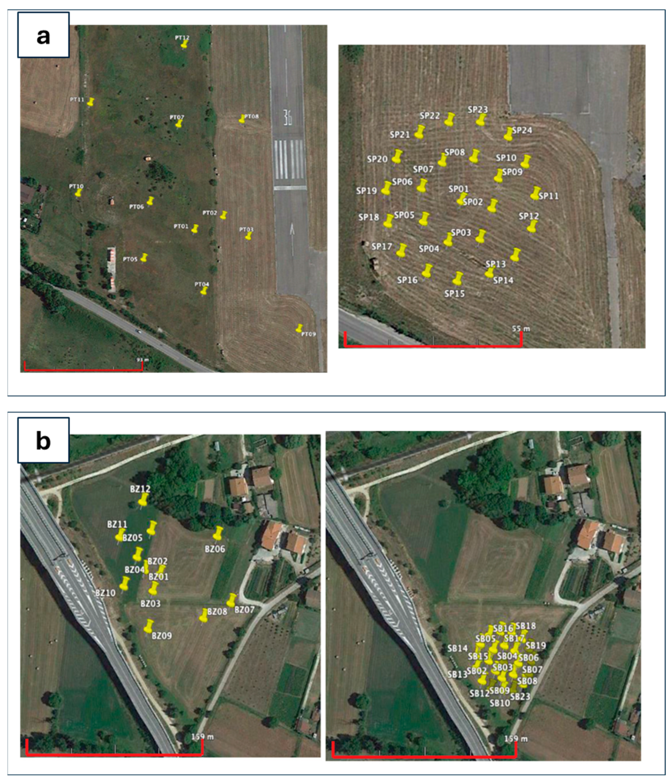
3.2. The 2D Microtremor Arrays

The array techniques are based chiefly on surface-wave theory [29] and are used for seismic site characterization [30]. In this study, a total of four bidimensional microtremor arrays were acquired in the Preturo–Sassa and Bazzano–Monticchio. More precisely, in each area, an array with 12 seismic stations (array BA) and another with 24 stations (SA array) were acquired (Figure 2). SA and BA are characterized by different array apertures. Array passive techniques are particularly suitable for investigations in even heavily anthropized areas and have the advantage of investigating lower frequencies than those generated by active sources, allowing greater investigation depths to be reached.

SA and BA are characterized by different instruments and array apertures (Figure 2). The BA array was made up of 12 “stand-alone” seismic stations equipped with Lennartz LE3d-5s triaxial sensors, connected to a 24-bit RefTek 130 digital digitizer. The Le3d-5s sensors have a sensitivity of 400 V/m/s and a usable frequency band ranging from 0.2 to 40 Hz. These characteristics make them particularly effective in the analysis of low frequencies, which are associated with greater investigation depths. The 12 stations were arranged on relatively large-opening irregular mesh layouts (spiral-like geometry), always with the aim of extending the investigation depths and decreasing spatial aliasing effects. The maximum opening of the array is approximately 250 m, with the aim of broadening the field of investigation towards low frequencies. The signals were acquired with a sampling rate of 250 Hz and for a simultaneous recording period at all stations of the array of 2 h.

The SA array involves 24 vertical sensors with a natural frequency of 4.5 Hz connected by cable to a 24-bit Geometrics Geode data acquisition device. The sensors of the SA array were installed on two concentric circles of radius 13 and 24 m, respectively. To improve the quality of data collection, the positioning of the stations of both arrays was obtained using a Leica differential GPS, which allows for a positioning error of less than 10 cm.

Given the use of three-component stations for the BA array, the H/V ratio was calculated at all stations to verify their spatial stability.

The HVSR ratios were interpreted in terms of Rayleigh-wave ellipticity and used for their joint inversion with the dispersion curves to reduce the uncertainties on the non-uniqueness of the subsoil model obtained. Data were analyzed using a three-component frequency–wavenumber (FK) analysis, which allows us to obtain both the dispersion curve and the ellipticity function for Rayleigh waves [31,32]. To improve the low frequency resolution, the SPAC technique (as implemented in Bettig et al. [33] for irregular geometry) was also applied. To obtain information at higher frequencies, to be associated with the shallower seismo-layers, the data recorded by the SA array were analyzed with FK array techniques. The dispersion curves obtained with the various analyses of the data acquired from the two arrays were then inverted to obtain the Vs velocity versus depth model. Combining the results of the BA and SA arrays, the analyzed frequency range of the dispersion curves, which can be used in the inversion process, ranges from 2 to 15 Hz and allows both the shallower and deeper seismo-layers of the model to be investigated with good resolution. The initial parameterization for the inversion was based on geological data acquired during the SM activities and boreholes available near the array location site.

3.3. Seismic Input

Following the Italian technical standards for construction NTC18 [7], seven natural accelerograms were selected as seismic inputs by using the online REXELite database based on a spectrum matching approach: https://itaca.mi.ingv.it/ItacaNet_40/#/rexel (accessed on 23 September 2024). REXELite is the simplified version of the Rexel database [34]. The used target response spectrum for L’Aquila town (latitude: 42.377; longitude: 13.310) is associated with a reference earthquake with a return period of 475 years on seismic bedrock (Vs > 800 m/s), horizontal topography, and 5% damping. The seismic inputs are a suite of seven real earthquakes selected by REXELite [35] and used in the numerical simulations for the estimation of the AFs.

In choosing them, based on the target spectrum, the following characteristics of the selected seismic events and recording sites were considered: (i) magnitude earthquake (Mw or Ml—interval): 5.5—7; (ii) focal mechanism: extensional fault; (iii) epicentral distance from the recording site: 0–30 km; (iv) recording site on seismic bedrock. Moreover, the used tolerance criteria between the target spectrum and the average value of the seven selected recordings are (i) period range considered for comparison: 0.1–1.1 s; (ii) upper tolerance: 30%; (iii) lower tolerance: 10%.

3.4. Computer Code Selection

In general, when subjected to cyclic loads, soils show nonlinear behavior characterized by hysteresis cycles on the shear stress Ƭ–shear strain γ plane. In numerical analyses, the possible procedures used to consider the nonlinear constitutive model of the soil are divided into [8,10]: (i) the equivalent linear approach and (ii) the incremental nonlinear approach. The equivalent linear approach consists of executing a series of linear analyses where the soil nonlinear behavior is described through the secant shear stiffness modulus G, given by the ratio τ/γ and the damping ratio D, which is proportional to the area of the hysteresis loop according to the Equation (1).

D = WD/4πWE

(1)

where D is the damping ratio, WD is the dissipated energy, and WE is the elastic energy [8].

Instead, the incremental nonlinear approach consists of the step-by-step integration of the equations of motion obtained according to a nonlinear constitutive model of the soil. This latter approach may exhibit some disadvantages. By way of example, it would not be possible to apply the superposition principle or other tools of linear analysis, such as transfer functions, Fourier analysis, etc. Furthermore, from a theoretical point of view, the solution of nonlinear differential equations presents greater complexity than linear ones [8]. When solving them by means of numerical methods, in several cases, their solution may present convergence problems and may require several iterations. Therefore, a purely nonlinear approach involves greater complexity of the algorithms and, in several cases, a considerable computational burden. As a result, codes that use this approach are more problematic to build and test. This translates into significant costs. To limit these drawbacks, many simulation codes use a linear equivalent approach [8]. According to this approach, a simulation code, starting from the reference earthquake, provided as an input accelerogram, integrates the equations of dynamic motion, based on initial values for the elastic moduli and damping ratios, to calculate the maximum strain γMax at every point of the model. From the effective strain values, given by γeff = α γMax (α is a coefficient dependent on the magnitude of the seismic event and variable in the range 0.6–0.7), the updated G and D values are achieved in each iteration through the curves describing the soil nonlinearity of shear modulus and damping ratio. Then, the current G and D estimates are compared with those achieved in the previous iteration. If both relative differences are less than the desired threshold, the iterations stop; otherwise, the calculation is repeated until this condition is satisfied.

To have a rational balance between the analysis accuracy and the computational burden, able to consider the nonlinear behavior of soil, the local seismic effects, and the geological complexity of the middle Aterno River basin, it was decided to resort to the 2D equivalent linear modeling. Although the equivalent linear approach introduces approximations into the calculations, it significantly reduces the complexity of elastic wave propagation equations and models in heterogeneous media with nonlinear viscoelastic behavior, allowing efficient software to be produced at limited costs and capable of being executed in a reasonable time range. Based on these considerations, for the AFs evaluation, the LSR 2D code by software house Stacec s.r.l. was used: https://www.stacec.com/lsr-2d_pp92.aspx (accessed on 23 September 2024). LSR 2D performs the 2D equivalent linear modeling by using the finite element approach, in the time domain and in total stresses and the Kelvin–Voigt model. In the 2D analysis with equivalent linear and concentrated masses approach, the subsoil model is discretized in a mesh with triangular or preferably quadrangular shape elements. Mesh generation is one of the most significant steps of the analysis, depending on both the accuracy of the solution and the computational burden [10]. In principle, the more mesh there is, the more accurate the solution, but the greater the time and memory required for processing. The use of an excessively coarse mesh results in a filtering of the high-frequency components (Figure 3).

The reason is that nodes too far apart cannot adequately model small wavelengths. Therefore, the height h of each element has to be chosen following Equation (2).

$$h\le \left({\displaystyle \frac{1}{8}}÷{\displaystyle \frac{1}{5}}\right) {\displaystyle \frac{V_s}{f_{max}}}$$

(2)

where ℎ is the mesh step; Vs is the shear-wave velocity; f_max is the maximum frequency considered in the analysis (usually equal to 20–25 Hz).

In this case study, the mesh generation was built with an adaptive approach so as to preserve computational resources in favor of the control points identified for obtaining the output results. The mesh step would increase from higher values starting from bedrock (equal to 4 m) and then level off at lower values (equal to 1 m) in the proximity of the control points. The overall balance is expressed by the following system of Equation (3).

$$M\ddot{u}+C\dot{u}+Ku=-M{a}_g$$

(3)

where u is the vector of nodal displacements; M, K, and C refer, respectively, to the matrix of masses, stiffness, and damping; a_g is the time history of the acceleration input. Equation (3) is solved by direct integration in the time domain with the Newmark method and with the CAA method (Constant Average Acceleration), which is stable and does not introduce any numerical damping. The seismic motion input a_g is applied simultaneously to the nodes of the bedrock base in the form of P and S waves with vertical propagation.

The dissipative properties of the soil are modeled through the matrix dissipation C. It derives from the assembly of the dissipation matrices of the individual elements calculated according to the complete Rayleigh Equation (4).

$$C_i={\alpha }_{Ri}{M}_i+{\beta }_{Ri}{K}_i$$

(4)

where α_Ri and β_Ri are the Rayleigh coefficients, C_i is the damping matrix, M_i is the mass matrix, and K_i is the stiffness matrix.

The adoption of the Rayleigh equations involves frequency-dependent damping, which can appreciably affect the modeling results. To reduce this effect, LSR 2D uses Rayleigh coefficients calculated according to two natural frequencies of soil deposit, ωn and ω_m (Equations (5) and (6)).

$${\alpha }_{Ri}={\xi }_i {\displaystyle \frac{ 2 {\omega }_m· {\omega }_n}{{\omega }_m+{\omega }_n}}$$

(5)

$${\beta }_{Ri}={\xi }_i{\displaystyle \frac{ 2 }{{\omega }_m+{\omega }_n}}$$

(6)

where ξ_i is the viscous damping ratio of the i-th element; ω_m = ω₁, the first natural vibration frequency of soil deposit; ω_n = n ω₁, where n is the odd integer that approximates by excess the predominant frequency ratio of the seismic input ω_IN and frequency ω₁.

The software LSR 2D requires as input, for each soil, the following parameters: (i) the volume weight; (ii) the shear modulus; (iii) the damping at low strain; (iv) the Poisson’s ratio; (iv) the G/G₀ vs. γ and D vs. γ curves; (v) the constant α for the calculation of the characteristic value of the shear deformation starting from the maximum value of γ (t) (typically equal to 0.65).

The code LSR 2D provides the following as output: (i) the maximum accelerations on all nodes; (ii) the maximum tangential stresses and strains in each element; (iii) the acceleration time history in the selected nodes (vertical and horizontal components).

3.5. Third-Level MS Mapping

Many geological sections were elaborated, and 2D simulations were carried out (n. 15) using the LSR 2D application. The sections were traced to cross most of the SM microzones of the pilot areas and the most significant geological boundaries (fault contacts, alluvial terrace scarps, landslides, anthropic deposits, etc.). Moreover, the sections were located close to the geophysical investigations (above all microtremor measurements and down-hole tests) and boreholes to better constrain the subsoil model. They start and end at least 400 m outside the extremes of the section, almost always located in the seismic bedrock, so as to minimize in the simulations the edge phenomena due to the lateral dispersion of the seismic energy. Orthogonal sections have also been elaborated for checking with the simulations of possible 2D phenomena due to seismic directionality.

Along the sections, the calculated point values and the class values of the AFs between 0.1 and 0.5 s were reported, considering this to be the most important period interval of the three required. The highest value within the microzone calculated along all the sections was chosen as the AF value for the 0.1–0.5 s range to be assigned to the third-level microzone after excluding anomalous AF outliers. An anomalous value is defined as a value that is particularly different from the surrounding area (two or more class differences) and does not have substantial geological justifications for its maintenance. The AFs for the other two periods to be assigned to the microzone (0.4–0.8 s and 0.7–1.1 s) are also computed and refer to the same progressive along the section of the AF of the 0.1–0.5 s period.

For each microzone, its output spectrum is that of the highest AF (0.1–0.5 s) calculated with 2D simulations for that microzone. This output spectrum is in pseudo-acceleration and corresponds to the average obtained from the seven individual spectra.

As a first approximation, it was decided to maintain the boundaries of the first-level microzone (named MOPS sensu SM Working Group [6], i.e., homogeneous seismo-stratigraphic microzone at 15,000–10,000 scale); therefore, in the case of two different MOPS having values within the same class of AFs, to keep them separate and thus map two third-level microzones with AFs of the same class but with different single reference values. In cases where the same first-level microzone presents two different classes of contiguous AF values, it was decided not to subdivide the MOPS into two third-level microzones, with the MOPS boundary corresponding to that of the microzone. The AF of the third-level microzone is the highest one calculated from the 2D simulations within the MOPS, as suggested by the SM Working Group [36]. This procedure is innovative and possibly provides a methodological proposal for the current Italian legislation on SM.

Instead, in the case of the same (first-level) MOPS represented by two or more non-contiguous AF classes, it was decided to divide the MOPS into two or more third-level microzones, with geological differentiation based on the points of divergence within the geological sections. These differences can be related within the MOPS to both variations in thickness and geometry of the same lithotechnical units and topographic variations in the MOPS.

In order not to make too many changes to the MOPS, it was decided to operate approximations when the boundary between two classes of AFs is very close to the boundary of two microzones but does not turn out to be the same, remaining within the calculation distance of the AFs along the sections (in our case 40–80 m).

Finally, for some microzones not covered by 2D simulations, 1D ones were performed with LSR 2D and Strata code [37].

4. Results

Following the Italian technical standards for construction NTC18 [7], seven natural accelerograms were selected as seismic inputs [34].

Figure 4 illustrates the set of seven accelerograms, complying with the criteria described in Section 3.3, which were utilized as input for 1D and 2D numerical simulations of the local seismic response.

The thick grey curve in the figure denotes the spectrum constituted by the medians of the values relating to the seven spectra for each period value. The regulation NTC18 requires that the values of this average spectrum do not differ by more than 30% in excess or 10% in defect from the target spectrum provided for by the above mentioned regulation [7]. The latter is calculated by the REXELite application according to the parameters illustrated in Section 3.3.

The geological units reported in Table 2 were characterized from a geophysical (Vs, Poisson’s ratio) and geotechnical (unit weight, G/G₀-γ and D-γ decay curves) point of view starting from the numerous seismic site characterization and local seismic response studies performed in the L’Aquila area for SM and research studies to which we refer [31,38,39,40] (Figure 5;

Table 3. Seismo-stratigraphic characteristics of the units used in all the numerical simulations.

Unit Code (+)	Vs (m/s)	Unit Weight (kN/m3)	Poisson’s Ratio	G/G0-γ and D-γ Decay Curves
ant	250	17	0.2	gravel medium model by [42]
fra	300	20	0.4	gravel medium model by [42]
fal	300	20	0.4	gravel medium model by [42]
all3	sand: 250 gravel: 300	19	0.2	sand model (upper–lower) by [41] gravel medium model by [42]
col	250	19	0.2	sand model (upper–lower) by [41]
at3	400	19	0.2	gravel medium model by [42]
at2	400	19	0.2	gravel medium model by [42]
dbf	800	20	0.2	model by [44]
at1	500	21	0.2	gravel medium model by [42]
ver	1200	21	0.2	elastic linear (damping: 0.5%)
all2	450 (Preturo–Sassa area) 450 (0–30 m) 600 (30–60 m) 700 (60–120 m) 750 (110–160 m) 800 (>160 m) (Bazzano–Monticchio area)	19	0.2	experimental data by sample S3 C3 Cese di Preturo [43]
all1	800	20	0.2	gravel medium model by [42]
UAP, UAM, UAM3, UAM1b	800	22	0.2	elastic linear (damping: 0.5%)
carbonate rocks SCZ, CBZ, etc.	1250	22	0.2	elastic linear (damping: 0.5%)

(+) Acronym of unit code by Abruzzo Seismic Microzonation Working Group [25].

).

The subsoil model for the Presturo–Sassa area was reconstructed through the integrated use of geological and borehole data, single-station microtremor previous studies [11], and new two-dimensional passive microtremor array measurements (Figure 2a and Figure 6), which enabled us to estimate the shear wave velocity profile for this area (Figure 7).

The values of the geophysical and geotechnical parameters reported in Table 3, used for the numerical simulations, are average values obtained from a large number of on-site investigations acquired on the wide area of LAB.

Also, in the area of Bazzano–Monticchio, two passive two-dimensional arrays were acquired with similar geometry used in Preturo (via 12 and 24 seismic stations, respectively, in Figure 2b).

Figure 8 illustrates the HVSR plots of the Bazzano array (12 stations configuration); f₀, f₁, and f₂ resonance frequencies can be noted for 0.4 Hz, 0.8–2 Hz, and 4–5 Hz, respectively. Furthermore, two-dimensional array measurements enabled us to estimate the shear wave velocity profile for this area (Figure 9).

Figure 10 and Figure 11 illustrate the results of the 1D and 2D numerical simulations conducted on the basis of the subsoil models achieved for the Preturo–Sassa and Bazzano–Monticchio areas. The red, green, and blue curves denote AFs in the period ranges of 0.1–0.5 s, 0.04–0.8 s, and 0.7–1.1 s, respectively. The diamond symbol refers to AFs calculated with 1D simulation for comparison with the results of 2D simulations. The formations denoted by SCZ, UAP, UAM1b, UAM3, and CBZ are carbonatic and terrigenous units showing bedrock characteristics (Vs > 800 m/s). A detailed description of all units is reported in Table 1, Table 2 and Table 3. In several areas in the illustrated sections, a swap between the curves of different colors is visible, indicating a shift of the frequencies most affected by amplification from higher to lower values and vice versa.

5. Discussions

5.1. The Subsoil Model

Traditional Near-Surface Geophysics methods, like down-hole, MASW, etc., often struggle to penetrate beyond 30 m below ground level. In sedimentary basins with deep seismic bedrock, as in the presented case study, more powerful techniques capable of reaching significant depths are necessary. The 2D microtremor array method offers a reliable solution for such scenarios. This technique, innovative within SM studies, provides quite rapid data acquisition and interpretation, thereby reducing costs. However, to enhance geological interpretation, it is crucial to complement the seismic array results with borehole logs, as illustrated in the presented case study.

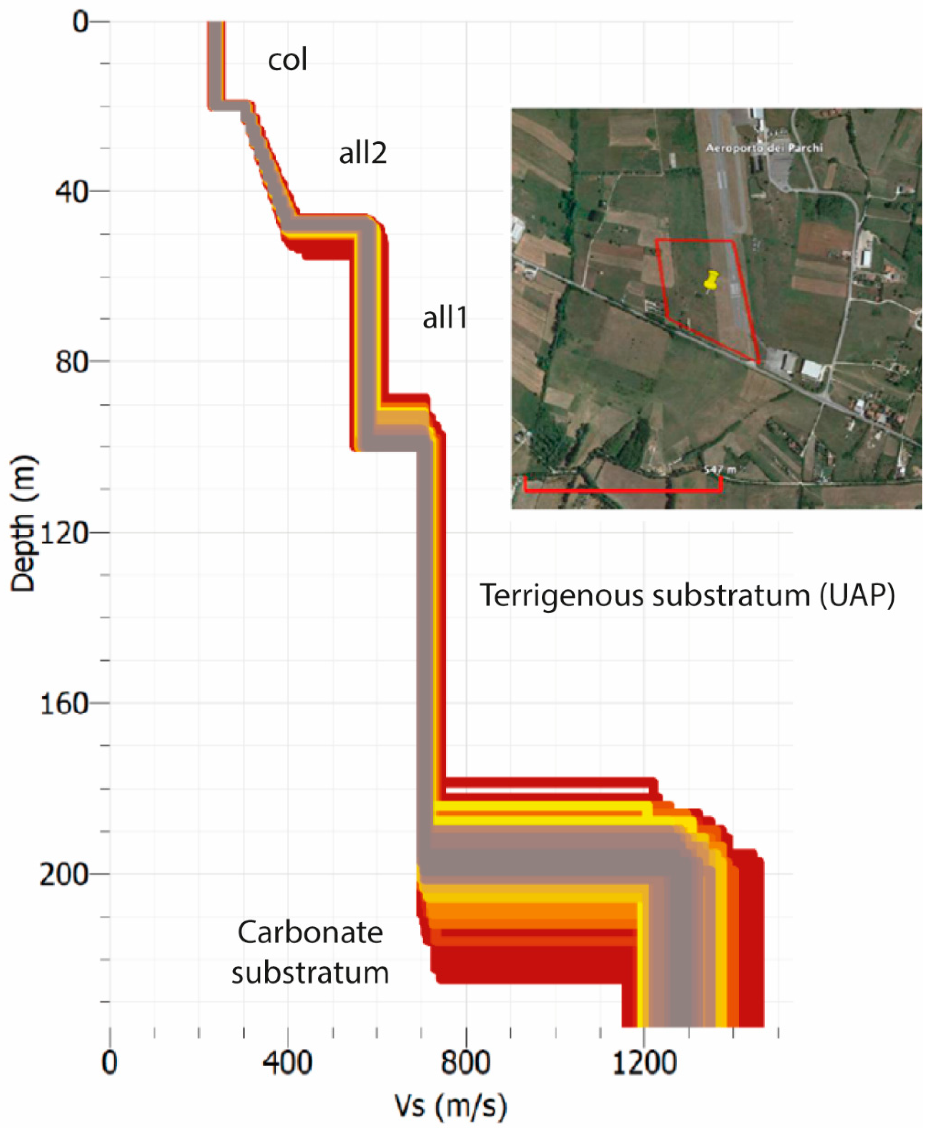
5.1.1. Preturo–Sassa Area

The geological model of the subsoil was reconstructed through (i) detailed geological and geomorphological surveys integrated with the study of (ii) boreholes dug in the area and (iii) passive microtremor acquired with single-station measurements [11] useful for defining the seismo-stratigraphy and the buried morphology of LAB, and (iv) geophysical investigations acquired ex novo (two-dimensional passive microtremor array measurements).

The main seismic impedance contrasts in the Preturo–Sassa area correspond mainly to the unit boundaries at the top and bottom of all2 (Madonna della Strada pelitic–sandy formation, Table 1, Table 2 and Table 3). From microtremor analysis, we observe three resonance frequencies: f₀, f₁, and f₂. The resonance frequencies f₁, equal to 1.0–1.5 Hz, are induced by the impedance contrast between all2 and all1 (Colle Cantaro Formation) or the geological substrate (UAM, UAP, CBZ, etc.) and all1 and the underlying geological substrate (Table 1, Table 2 and Table 3; Figure 6). The resonance frequencies f₂, equal to 10 Hz, are instead due to the very shallow contrast between mainly the recent deposit (e.g., all3, ant, fra, fal, col units) onto (i) all2; (ii) rocky Pleistocene breccia (dbf, ver); (iii) the terraced fluvial units (e.g., at1, at2, at3); or (iv) the geological substrate (Table 1, Table 2 and Table 3; Figure 6). The frequency f₀ is visible only in some of the H/V curves of Figure 6a, with rather dispersed values in the range 0.2–0.7 Hz, which gives a disordered feature to the envelope of these curves. This frequency value is associated with deeper seismic impedance contrasts involving the rocky substrate. Its variability is likely due to two-dimensional effects related to the occurrence of faults that confer to the basement an articulated geometry and lateral variations in composition.

Through the definition of an empirical relationship between the resonance frequency and the thickness of the Plio–Quaternary basin covering unit, the isobaths of the geological substrate were reconstructed [11], which highlighted an irregular trend of the pre-Plio–Quaternary substrate, indicating the presence of a very complex buried paleo morphology, with high morphological areas alternating with buried paleovalleys and slopes. From the observation of the isobaths reported by Nocentini et al. [11], it is noted mainly that the basin generally has depths greater than 60 m, with the most depressed area located between Preturo, the Preturo airport, and the Aterno river, where the substrate is found at a maximum depth of 120 m. This depression then extends in an N-S direction below the Raio plain and then orients itself in an E-W direction to form a narrow paleovalley with a depth between 80 and 60 m.

The data array processing based on the joint inversion of dispersion and H/V curves made it possible, in the Preturo airport site, to reconstruct the shear-wave velocity (Vs) versus depth profile. The profile highlighted a series of sharp Vs changes which may have correspondence with the geological setting (Figure 7): (i) at 20 m bgl, the boundary between col (Vs = 250 m/s) and the underlying unit at1/all2 (Vs = 450–500 m/s); (ii) at 50 m bgl, the boundary between all2 (Vs = 450 m/s) and the underlying unit all1 (Vs = 800 m/s); (iii) at 100 m bgl, the boundary between all1 and the geological substrate made up of UAP (Vs = 700–800 m/s); (iv) at 200 m bgl, the boundary, within the geological substrate, between UAP-UAM and the carbonate units (Miocene CBZ or Mesozoic units) (Vs = 1250–1300 m/s). Therefore, the above-mentioned arrays also highlighted, compared to single-station microtremor measurements [11], a deep impedance contrast within the geological substrate. This substratum should correspond to the f₀ in the range of 0.4–0.7 Hz (Figure 6).

The Vs values obtained with the array for the shallow units (e.g., col, ant, and all3), the all2, all1, UAP-UAM, and carbonate units are substantially in agreement with those estimated from in hole investigations [38,39] (Table 3).

Table 4. Comparison between the resonance frequencies obtained with the 2D microtremor array (Figure 2a and Figure 6) and those evaluated by using Equation (1).

Main Seismic Boundary (+)	Vs (m/s)	Thickness (m)	Depth (m bgl)	Average Vs (m/s) with Respect to Depth	Evaluated Resonance Frequency (Hz)	Measured Resonance Frequency (Hz)
bottom col	200	20	20	200	2.5	2.5–10
bottom all2	350	30	50	310	1.5	1.0–1.5
bottom all1	500	50	100	405	1.0	1.0–1.5
bottom UAP	700	100	200	552	0.7	0.4–0.7

(+) acronym of unit code by Abruzzo Seismic Microzonation Working Group [25].

shows the measured resonance frequencies and those estimated using the well-known 1D formula [45]:

f = Vs/(4H)

(7)

where f is the resonance frequency induced by the seismic impedance contrast of the seismo-layer of thickness H and velocity Vs. H was estimated by the stratigraphic log of the borehole P36 (Figure 6) and the 2D array analysis (Figure 7). Vs was estimated by 2D array analysis. A fine correspondence between these two values (evaluated and measured resonance frequencies) can be observed, reinforcing the goodness of the seismo-stratigraphic model used for the numerical simulations.

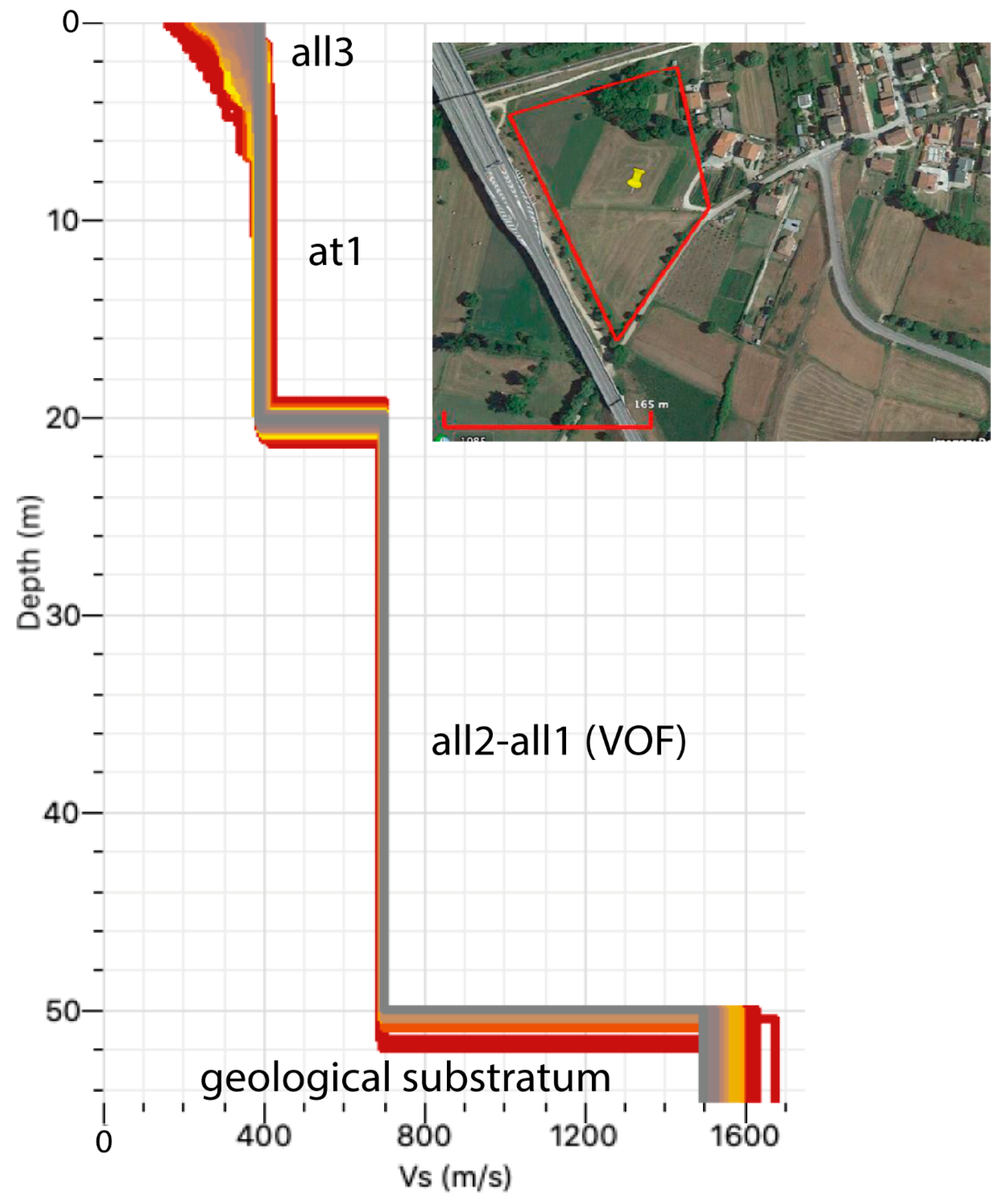
5.1.2. Bazzano–Monticchio Area

Also, for the Bazzano–Monticchio area, the data processing enabled us to reconstruct the Vs velocity profile, which highlighted four layers: A (0–8 m, Vs = 275 m/s), B (8–20 m, VS = 400 m/s), C (20–50 m, Vs = 680 m/s), and D (50–54 m, Vs = 1500 m/s) (Figure 9). Layer A corresponds to the all3 unit; B corresponds to the at1 unit, also based on the stratigraphic log of a nearby borehole; C corresponds to the deeper layers of all2 unit and all1 unit; and D corresponds to the geological substratum (Figure 9).

Table 5. Comparison between the resonance frequencies obtained with the 2D microtremor array (Figure 8) and those evaluated by using Equation (7).

Main Seismic Boundary (+)	Vs (m/s)	Thickness (m)	Depth (m bgl)	Average Vs (m/s) with Respect to Depth	Evaluated Resonance Frequency (Hz)	Measured Resonance Frequency (Hz)
bottom all3	250	4	4	250	16	-
bottom at1	500	16	20	450	5.6	4–5

(+) Acronym of unit code by Abruzzo Seismic Microzonation Working Group [25].

shows the measured resonance frequencies (Figure 8) and those estimated using the simplified Equation (7). H and Vs were obtained by the stratigraphic log of nearby boreholes and the geophysical investigations acquired in the area (Table 3). Also, in this case, a fine correspondence between these two values (evaluated and measured resonance frequencies) can be observed for the shallow seismic layers (A and B).

The geological interpretation of the deeper layers (C and D) appears to be more doubtful due to the lack of precise information close to the array site (e.g., boreholes, etc.) and the variability of the geology near the basin edge.

Additionally, for the Bazzano–Monticchio area, the Vs values obtained with the array are substantially in agreement with those estimated from in situ investigations (Table 2 and Table 3).

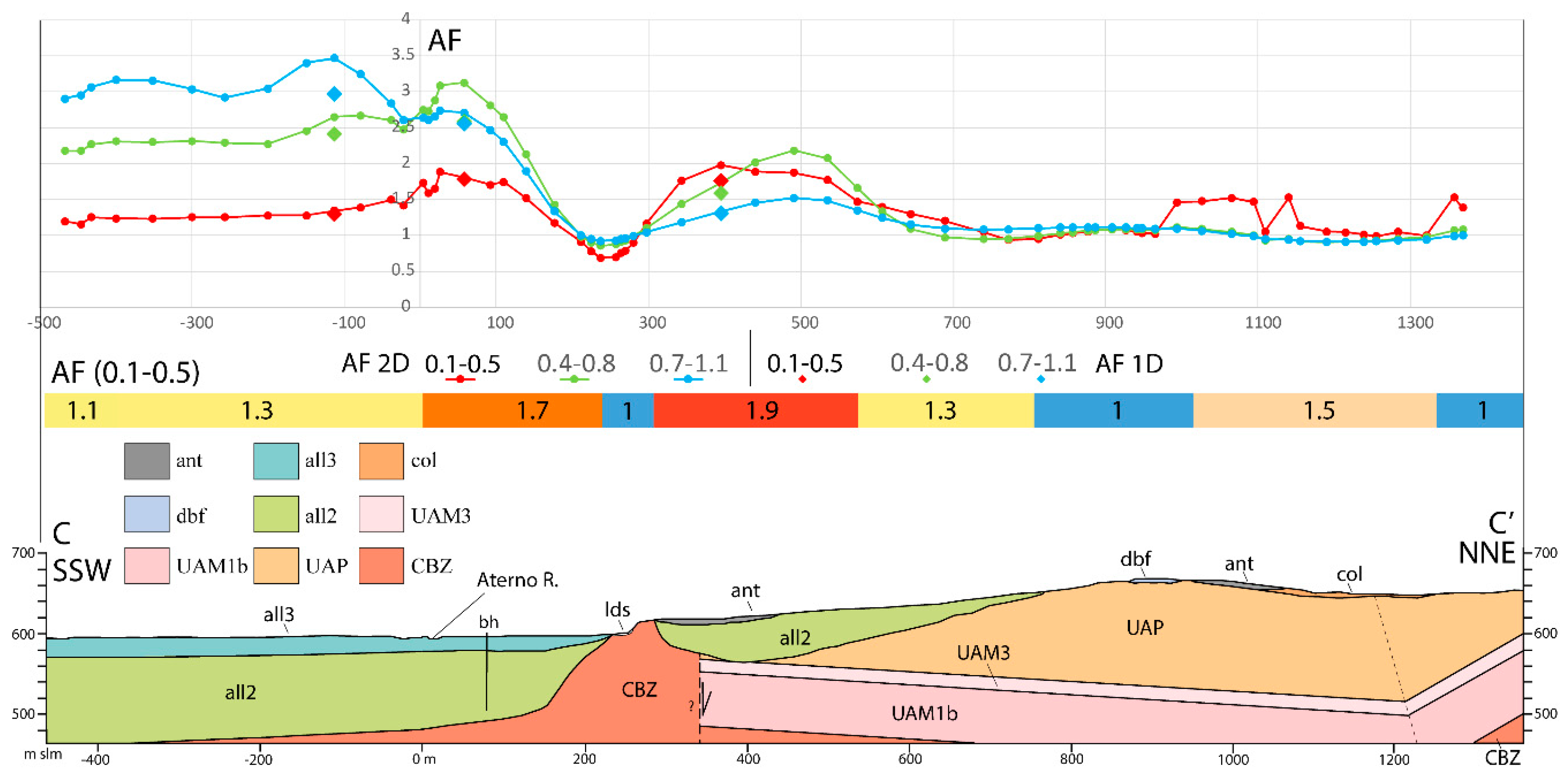
5.2. The Numerical Modelling and Third-Level SM Deliverables

The AFs were calculated by means of the LSR 2D code along the sections every 30–50 m, with three calculated points located in a zone of 70 m as a minimum and 120 m as a maximum. After the calculation of AFs, a three-data filtering was performed to make the trend of the AF values homogeneous along the progressives of the section (Figure 10 and Figure 11). Since 2D simulations were performed for each microzone, more points were available in which the AFs were calculated. Therefore, based on an evaluation in favor of safety and subject to expert judgment, the AF of the microzone is the highest of those calculated within the microzone for the period interval 0.1–0.5 s, and the accelerograms and response spectra representative of the microzone refer to those of the AF attributed to it.

The following documents were produced for the Preturo–Sassa and Bazzano–Monticchio areas (L’Aquila Municipality): (i) third-level SM maps of the AFs for the three-period intervals (0.1–0.5 s, 0.4–0.8 s, 0.7–1.1 s) at 1:5000 scale; (ii) database organized by using the CNR-IGAG plugin “MzS Tools” operating on QGIS ver. 3.22 [46].

For each microzone, the following data were also produced: (i) n. three AFs, one for each period interval (0.1–0.5 s, 0.4–0.8 s, 0.7–1.1 s); (ii) n. seven natural accelerograms used as seismic input for the 2D modeling; (iii) n. seven elastic acceleration response spectra at 5% damping (output spectra) at the surface, one for each input accelerogram; (iv) the representative output spectrum of the microzone, i.e., the average spectrum of the seven above-mentioned spectra; (v) the Vs,eq value and the related subsoil category according to CS.LL.PP. [7]. The Vs,eq value was calculated for each microzone, using the average thickness of the seismic layers and the relative values of Vs used for the modeling.

In Figure 12, as an example, the third-level SM map of Preturo is reported for the period interval of 0.1–0.5 s.

5.3. Model Validation

To evaluate the reliability of the calculated AFs, quality control was performed by comparing them with the geological maps. Indeed, it has been noted that the distribution of the calculated AFs is congruent with the geological background. In fact, along the sections, a rough correspondence between the boundaries of the AF classes and the geological units is observed, although, in some microzones, it is not always clearly evident. Further, for the outcropping geological units, the AF values vary within a narrow range. It has also been observed that the AF values are conditioned by the shallower seismic impedance contrast. However, these observations agree with the theory [8,45] and, therefore, lead us to believe that the AFs obtained with the simulations are to be considered reliable. Moreover, in most of the studied areas, considering the sufficient correlation between the AFs and the geology background, the boundaries of the third-level SM microzones were spatially extended based on the geological unit boundaries and via expert judgment [47].

To verify the presence of basin effects, we compared the AFs obtained with the 1D simulation with those calculated with the 2D ones in the same site. In several cases, 2D basin effects were detected, as the AFs calculated in the basin center with 1D modeling were lower than the AFs estimated with 2D one (Figure 10). Moreover, near the slope break between the reliefs and the Aterno R. plain, the AF values calculated with 2D simulation are higher with respect to the surrounding areas and are lower than those estimated with 1D modeling. This behavior would probably be attributable to the 2D basin-edge effect [45] (Figure 10).

For almost all the sections of the Bazzano–Monticchio area crossing the Aterno R. plain, the AF values increase for the intervals of the higher periods, i.e., a shift of the seismic energy towards higher periods is noted (lower frequencies) (Figure 11). This behavior seems to be linked to the 2D effect because the FAs calculated in points located on the Aterno R. plain with a 1D modeling are generally lower than the FAs estimated with the 2D one [8].

6. Conclusions

This study presents the results of a third-level Seismic Microzonation project conducted in pilot areas within the municipality of L’Aquila, Italy. The study area is characterized by significant seismic activity, as evidenced by the 2009 L’Aquila earthquake (Mw 6.3) and the 2016 Central Italy seismic sequence (Mw 6.0 and 6.5). This research produced detailed numerical maps at a scale of 1:1500 to support sustainable urban and territorial planning.

A novel approach was adopted, integrating traditional geophysical and geotechnical subsurface characterization techniques with the acquisition of 2D microtremor arrays and extensive 2D numerical simulations of local site response. The combined use of 2D microtremor arrays and geological and geophysical data enabled more accurate quantification of subsurface characteristics, such as bedrock depth and Vs velocities of surface soils. Comparisons between 2D and 1D numerical simulations highlighted the presence of basin and basin-edge effects in several areas.

The proposed approach may lead to a significant advancement in third-level microzonation, as it allows for more realistic modeling of local site response, which, in turn, can lead to improved structural design of buildings. Therefore, this contribution represents a step forward towards sustainable construction and effective urban and land management.

References

1. Adhikari, S.R.; Molnar, S.; Wang, J. Seismic microzonation mapping of Greater Vancouver based on various site classification metrics. Front. Earth Sci. 2023, 11, 1221234. [Google Scholar] [CrossRef]
2. Bıçakcı, G.B.; Özçep, F.; Karabulut, S.; Cengiz, M. The Importance of seismic microzonation under the threat of an earthquake of the north anatolian fault in nilüfer, bursa, turkey. J. Appl. Geophys. 2024, 229, 105489. [Google Scholar] [CrossRef]
3. Chen, G.; Magistrale, H.; Rong, Y.; Cheng, J.; Ahmet Binselam, S.; Xu, X. Seismic site condition of Mainland China from geology. Seism. Soc. Am. 2021, 92, 998–1010. [Google Scholar] [CrossRef]
4. Fäh, D.; Rüttener, E.; Noack, T.; Kruspan, P. Microzonation of the city of Basel. J. Seism. 1997, 1, 87–102. [Google Scholar] [CrossRef]
5. Licata, V.; Forte, G.; d’Onofrio, A.; Santo, A.; Silvestri, F. A multi-level study for the seismic microzonation of the Western area of Naples (Italy). Bull. Earthq. Eng. 2019, 17, 4711–4741. [Google Scholar] [CrossRef]
6. SM Working Group. Guidelines for Seismic Microzonation, Conference of Regions and Autonomous Provinces of Italy; Civil Protection Department: Rome, Italy, 2008; pp. 1–124. Available online: https://www.centromicrozonazionesismica.it/documents/18/GuidelinesForSeismicMicrozonation.pdf (accessed on 6 September 2024).
7. CS.LL.PP. Aggiornamento delle Norme Tecniche per le Costruzioni [Improvement of Technical Standards for Construction]. Gazzetta Ufficiale della Repubblica Italiana 2018; p. 42. Available online: https://www.gazzettaufficiale.it/eli/id/2018/2/20/18A00716/sg (accessed on 6 September 2024).
8. Kramer, S.L. Geotechnical Earthquake Engineering; Pearson Education India: Chennai, India, 1996. [Google Scholar]
9. Sucuoglu, H.; Akkar, S. Basic Earthquake Engineering: From Seismology to Analysis and Design; Springer: Cham, Switzerland, 2014; Volume 1, ISBN 9783319010250. [Google Scholar]
10. Yoshida, N. Seismic Ground Response Analysis; Springer: Berlin/Heidelberg, Germany, 2015; Volume 36, ISBN 978-94-017-9460-2. [Google Scholar]
11. Nocentini, M.; Asti, R.; Cosentino, D.; Durante, F.; Gliozzi, E.; Macerola, L.; Tallini, M. Plio-Quaternary geology of L’Aquila–Scoppito Basin (Central Italy). J. Maps 2017, 13, 563–574. [Google Scholar] [CrossRef]
12. Chiarabba, C.; Amato, A.; Anselmi, M.; Baccheschi, P.; Bianchi, I.; Cattaneo, M.; Cecere, G.; Chiaraluce, L.; Ciaccio, M.G.; De Gori, P.; et al. The 2009 L’Aquila (central Italy) MW6.3 earthquake: Main shock and aftershocks. Geophys. Res. Lett. 2009, 6, 18308. [Google Scholar] [CrossRef]
13. Wang, L.; Nagarajaiah, S.; Zhou, Y.; Shi, W. Seismic performance improvement of base-isolated structures using a semi-active tuned mass damper. Eng. Struct. 2022, 271, 114963. [Google Scholar] [CrossRef]
14. Wang, L.; Zhou, Y.; Shi, W. Seismic Response Control of a Nonlinear Tall Building Under Mainshock-Aftershock Sequences Using Semi-Active Tuned Mass Damper. Int. J. Struct. Stab. Dyn. 2023, 23, 2340027. [Google Scholar] [CrossRef]
15. Bisch, P.; Carvalho, E.; Degee, H.; Fajfar, P.; Fardis, M.; Franchin, P.; Kreslin, M.; Pecker, A.; Pinto, P.; Plumier, A.; et al. Eurocode 8: Seismic Design of Buildings Worked Examples; Publications Office of the European Union: Luxembourg, 2012; Available online: http://www.jrc.ec.europa.eu/ (accessed on 6 September 2024).
16. Carminati, E.; Lustrino, M.; Cuffaro, M.; Doglioni, C. Tectonics, magmatism and geodynamics of Italy: What we know and what we imagine. J. Virtual Explor. 2010, 36, 9. [Google Scholar] [CrossRef]
17. Cavinato, G.P.; De Celles, P.G. Extensional basins in the tectonically bimodal central Apennines fold-thrust belt, Italy: Response to corner flow above a subducting slab in retrograde motion. Geology 1999, 27, 955–958. [Google Scholar] [CrossRef]
18. Barchi, M.; Galadini, F.; Lavecchia, G.; Messina, P.; Michetti, A.M.; Peruzza, L.; Pizzi, A.; Tondi, E.; Vittori, E. Sintesi Delle Conoscenze Sulle Faglie Attive in Italia Centrale: Parametrizzazione ai Fini Della Caratterizzazione Della Pericolosità Sismica [Summary of Knowledge on Active Faults in Central Italy: Parameterization for the Purposes of Characterizing Seismic Hazard]; CNR Gruppo Nazionale per la Difesa dai Terremoti: Roma, Italy, 2000; p. 62. Available online: https://www.researchgate.net/profile/Paolo-Messina-4/publication/235233363_Sintesi_delle_Conoscenze_Sulle_Faglie_Attive_in_Italia_Centrale_Parametrizzazione_ai_Fini_della_Caratterizzazione_della_Pericolosita_Sismica/links/02e7e53287abc91669000000/Sintesi-delle-Conoscenze-Sulle-Faglie-Attive-in-Italia-Centrale-Parametrizzazione-ai-Fini-della-Caratterizzazione-della-Pericolosita-Sismica.pdf (accessed on 6 September 2024).
19. Boncio, P.; Lavecchia, G.; Pace, B. Defining a model of 3D seismogenic sources for seismic hazard assessment applications: The case of central Apennines (Italy). J. Seism. 2004, 8, 407–425. [Google Scholar] [CrossRef]
20. Devoti, R.; Pietrantonio, G.; Pisani, A.; Riguzzi, F.; Serpelloni, E. Present day kinematics of Italy. J. Virtual Explor. 2010, 36, 2. [Google Scholar] [CrossRef]
21. Pondrelli, S.; Salimbeni, S.; Ekstrom, G.; Morelli, A.; Gasperini, P.; Vannucci, G. The Italian CMT dataset from 1977 to the present. Phys. Earth Planet. Inter. 2006, 159, 286–303. [Google Scholar] [CrossRef]
22. Galadini, F.; Galli, P. Active tectonics in the central Apennines (Italy) and input data for seismic hazard assessment. Nat. Hazards 2000, 22, 225–270. [Google Scholar] [CrossRef]
23. Sciortino, A.; Marini, R.; Guerriero, V.; Mazzanti, P.; Spadi, M.; Tallini, M. Satellite A-DInSAR pattern recognition for seismic vulnerability mapping at city scale: Insights from the L’Aquila (Italy) case study. GIScience Remote Sens. 2024, 61, 1. [Google Scholar] [CrossRef]
24. Sciortino, A.; Guerriero, V.; Marini, R.; Spadi, M.; Mazzanti, P.; Tallini, M. Geological and Hydrogeological Drivers of Seismic Deformation in L’Aquila, Italy: Insights from InSAR Analysis. Geomat. Nat. Hazards Risk 2024, 15, 2362395. [Google Scholar] [CrossRef]
25. Abruzzo Seismic Microzonation Working Group. Standard di Rappresentazione Cartografica e Archiviazione Informatica. Specifiche Tecniche per la Redazione Degli Elaborati Cartografici ed Informatici Relativi al Primo Livello Delle Attività di Microzonazione Sismica [Standard of Cartographic Representation and Geodatabase Archiving. Technical Specifications for First Level Seismic Microzonation Mapping], ver. 1.2, L’Aquila. 2012. Available online: https://protezionecivile.regione.abruzzo.it/agenzia/files/rischio%20sismico/microzonazione/OPCM3907/LineeGuidaMS_v1_2_ONLINE2.pdf (accessed on 6 September 2024).
26. APAT (2006)–Sheet 359 “L’Aquila”. APAT–Servizio Geologico d’Italia e Regione Abruzzo–Servizio Difesa del Suolo, S.EL.CA., Firenze. Available online: https://www.isprambiente.gov.it/Media/carg/359_LAQUILA/Foglio.html (accessed on 6 September 2024).
27. APAT (2008)–Sheet 358 “Pescorocchiano”. APAT–Servizio Geologico d’Italia, S.EL.CA., Firenze. Available online: https://www.isprambiente.gov.it/Media/carg/358_PESCOROCCHIANO/Foglio.html (accessed on 6 September 2024).
28. Cosentino, G.; Pennica, F.; Tarquini, E.; Stigliano, F.; Coltella, M. Manuale per l’utilizzo del plugin “MzS Tools” con Licenza Creative Commons Attribuzione 4.0 Internazionale. 2022. Available online: https://github.com/CNR-IGAG/mzs-tools (accessed on 6 September 2024).
29. Tokimatsu, K. Geotechnical site characterization using surface waves. In Proceedings of the IS-Tokyo 95, The First International Conference on Earthquake Geotechnical Engineering, Tokyo, Japan, 14 November 1995. [Google Scholar]
30. Foti, S.; Parolai, S.; Bergamo, P.; Di Giulio, G.; Maraschini, M.; Milana, G.; Picozzi, M.; Puglia, R. Surface wave surveys for seismic site characterization of accelerometric stations in ITACA. Bull. Earthq. Eng. 2011, 9, 1797–1820. [Google Scholar] [CrossRef]
31. Di Giulio, G.; Gaudiosi, I.; Cara, F.; Milana, G.; Tallini, M. Shear-wave velocity profile and seismic input derived from ambient vibration array measurements: The case study of downtown L’Aquila. Geophys. J. Int. 2014, 198, 848–866. [Google Scholar] [CrossRef]
32. Lacoss, R.T.; Kelly, E.J.; Toksoz, M.N. Estimation of seismic noise structure using arrays. Geophysics 1969, 34, 21–38. [Google Scholar] [CrossRef]
33. Bettig, B.; Bard, P.-Y.; Scherbaum, F.; Riepl, J.; Cotton, F.; Cornou, C.; Hatzfeld, D. Analysis of dense array measurements using the modified spatial auto-correlation method (SPAC). Appl. Grenoble Area. Bol. Geofis. Teor. E Appl. 2001, 42, 281–304. Available online: https://epsc.wustl.edu/~ggeuler/reading/cam_noise_biblio/bettig_bard_scherbaum_riepl_cotton_cornou_and_hatzfeld_2001-bgta-analysis_of_dense_array_noise_measurements_using_the_modified_spatial_auto-correlation_method_spac_-_application_to_the_grenoble_area.pdf (accessed on 6 September 2024).
34. Iervolino, I.; Galasso, C.; Cosenza, E. REXEL: Computer aided record selection for code-based seismic structural analysis. Bull. Earthq. Eng. 2009, 8, 339–362. [Google Scholar] [CrossRef]
35. Sgobba, S.; Puglia, R.; Pacor, F.; Luzi, L.; Russo, E.; Felicetta, C.; Lanzano, G.; D’Amico, M.; Baraschino, R.; Baltzopoulos, G.; et al. REXELweb: A tool for selection of ground-motion records from the Engineering Strong Motion database (ESM). In Earthquake Geotechnical Engineering for Protection and Development of Environment and Constructions; CRC Press: Boca Raton, FL, USA, 2019; pp. 4947–4953. [Google Scholar]
36. SM Working Group. Informatic Representation and Archiving Standards. Seismic Microzonation. Version 4.2. Conference of Regions and Autonomous Provinces of Italy; Civil Protection Department: Rome, Italy, 2020; pp. 1–138. Available online: https://www.webms.it/sites/default/files/2018-06/StandardMS_4_2.pdf (accessed on 6 September 2024).
37. Kottke, A.R.; Rathje, E.M. Technical Manual for Strata; PEER Report 2008/10; Pacific Earthquake Engineering Research Center, University of California: Berkeley, CA, USA, 2009; pp. 1–103. [Google Scholar]
38. Cardarelli, E.; Cercato, M. Relazione Sulla Campagna D’indagine Geofisica per lo Studio Della Risposta Sismica Locale Della Città Dell’aquila, Prova Crosshole, Sondaggi S3-S4 [Report on the Geophysical Survey Campaign for the Study of the Local Seismic Response of the City of L’Aquila, Crosshole Test, Boreholes S3-S4]; Report for CERFIS; La Sapienza University of Rome: Roma, Italy, 2010; 13p. [Google Scholar]
39. Lanzo, G.; Tallini, M.; Milana, G.; Di Capua, G.; Del Monaco, F.; Pagliaroli, A.; Peppoloni, S. The Aterno Valley strong-motion array: Seismic characterization and determination of subsoil model. Bull. Earthq. Eng. 2011, 9, 1855–1875. [Google Scholar] [CrossRef]
40. Durante, F.; Di Giulio, G.; Tallini, M.; Milana, G.; Macerola, L. A multidisciplinary approach to the seismic characterization of a mountain top (Monteluco, central Italy). Phys. Chem. Earth Parts A/B/C 2017, 98, 119–135. [Google Scholar] [CrossRef]
41. Seed, H.B.; Wong, R.T.; Idriss, I.M.; Tokimatsu, K. Moduli and damping factors for dynamic analyses of cohesionless soils. J. Geotech. Eng. 1986, 112, 1016–1032. [Google Scholar] [CrossRef]
42. Rollins, K.M.; Evans, M.D.; Diehl, N.B.; Daily, W.D., III. Shear modulus and damping relationships for gravels. J. Geotech. Geoenvironmental Eng. 1998, 124, 396–405. [Google Scholar] [CrossRef]
43. MS-AQ Working Group. Seismic Microzonation for the Reconstruction of L’Aquila. 2010. Available online: https://www.protezionecivile.gov.it/it/pubblicazione/microzonazione-sismica-la-ricostruzione-dellarea-aquilana/ (accessed on 6 September 2024).
44. Modoni, G.; Gazzellone, A. Simplified theoretical analysis of the seismic response of artificially compacted gravels. In Proceedings of the 5th International Conference on Recent Advances in Geotechnical Earthquake Engineering and Soil Dynamics, San Diego, CA, USA, 26 May 2010. Paper No. 1.28a. [Google Scholar]
45. Lanzo, G.; Silvestri, F. Risposta Sismica Locale: Teoria ed Esperienze; Hevelius Edizioni: Benevento, Italy, 1999; pp. 1–159. [Google Scholar]
46. Cosentino, G.; Pennica, F. Manuale D’uso Del Plugin MzS Tools [MzS Tools Plugin User Manual]. 2022. Available online: https://mzs-tools.readthedocs.io/it/latest/intro.html (accessed on 6 September 2024).
47. Pergalani, F.; Pagliaroli, A.; Bourdeau, C.; Compagnoni, M.; Lenti, L.; Lualdi, M.; Madiai, C.; Martino, S.; Razzano, R.; Varone, C.; et al. Seismic microzoning map: Approaches, results and applications after the 2016-2017 Central Italy seismic sequence. Bull. Earthq. Eng. 2020, 18, 5595–5629. [Google Scholar] [CrossRef]
Figure 1. The study area of Preturo–Sassa (1) and Bazzano–Monticchio (2) (L’Aquila Municipality). The dotted yellow lines refer to sections A-A’, B-B’, and C-C’. In both sites (i.e., the Preturo airport and nearby Bazzano), 2D microtremor arrays were acquired.
Sustainability 16 08401 g001
Figure 2. (a) Vs array geometry for the Preturo site. (Left): array BA geometry with 12 stations; (right): array SA geometry with 24 stations. (b) Vs arrays geometry for the Bazzano site. (Left): array BA geometry with 12 stations; (right): array SA geometry with 24 stations.
Sustainability 16 08401 g002
Figure 3. Section B-B’ (Preturo–Sassa area): details of the mesh by LSR 2D code.
Sustainability 16 08401 g003
Figure 4. The seven seismic input accelerograms selected for this study by the REXELite database [34].
Sustainability 16 08401 g004
Figure 5. Decay curve G/G0–shear strain γ (%) (left) and damping curve D–shear strain γ (%) (right) obtained from: (a) sand model (upper–lower) by [41]; (b) gravel medium model by [42]; (c) resonant column and cyclic torsion test on sample S3 C3 (silty clay) sampled in the borehole S3 at 17.5–18.0 m bgl (Cese Preturo) [43]; (d) model by [44].
Sustainability 16 08401 g005
Figure 6. Geological section A-A’ (for the location, see Figure 1). In the section, the site (Preturo airport) of the microtremor arrays is located. For the explanation of the resonance frequencies (f0, f1, and f2), see the text. (a) HVSR curves for the 12 stations of the BA array; (b) an average of the HVSR values. The acronym P refers to the borehole. The log of P36, located near the microtremor arrays, is also reported.
Sustainability 16 08401 g006
Figure 7. Vs value vs. depth profile obtained through passive microtremor acquisition with two 2D arrays located at Preturo airport (see the location map). Also, the geological interpretation of the seismo-layers is reported (Table 1, Table 2 and Table 3).
Sustainability 16 08401 g007
Figure 8. (a) HVSR plots for the 12 stations of the array; (b) an average of the HVSR values (Bazzano array); f0, f1, and f2 resonance frequencies can be noted for 0.4 Hz, 0.8–2 Hz, and 4–5 Hz, respectively.
Sustainability 16 08401 g008
Figure 9. Vs value vs. depth profile obtained through passive microtremor acquisition with two 2D arrays consisting of 12 and 24 seismic stations, respectively, located at the Bazzano site (see the location map). Also, the geological interpretation of the layers is reported (Table 1, Table 2 and Table 3).
Sustainability 16 08401 g009
Figure 10. FA values, calculated through 2D modeling, for Preturo–Pagliare di Sassa area that is represented in section B-B’ (Figure 1). The diamond symbol refers to AF calculated with 1D simulation. The letters from A to E indicate the points of the section where the amplification factor was calculated with 1D modeling. bh: boreholes; SCZ and UAP: calcareous and terrigenous units belonging to the seismic bedrock; the other units refer to the Plio–Quaternary basin-filling detrital units (Table 1, Table 2 and Table 3). AF intervals: Class 1.0: AF < 1.05; Class 1.1: 1.05 ≤ AF > 1.25 (not present); Class 1.3: 1.25 ≤ AF > 1.45; Class 1.5: 1.45 ≤ AF > 1.65; Class 1.7: 1.65 ≤ AF > 1.85; Class 1.9: 1.85 ≤ AF > 2.05; Class 2.1: 2.05 ≤ AF > 2.25; Class 2.3: 2.25 ≤ AF > 2.45 (not present).
Sustainability 16 08401 g010
Figure 11. In the Bazzano–Monticchio area represented in section C-C’ (Figure 1), the AF values, calculated through 2D modeling, increase for the intervals of the higher periods, i.e., a shift of the seismic energy towards higher periods is noted (lower frequencies). The diamond symbol refers to AF calculated also with 1D simulation. bh: boreholes; lds: landslide; CBZ and UAM3, UAM1b, UAP: calcareous and terrigenous units belonging to the seismic bedrock; the other units refer to the Plio–Quaternary basin-filling detrital units (Table 1, Table 2 and Table 3). AF intervals: Class 1.0: AF < 1.05; Class 1.1: 1.05 ≤ AF > 1.25; Class 1.3: 1.25 ≤ AF > 1.45; Class 1.5: 1.45 ≤ AF > 1.65; Class 1.7: 1.65 ≤ AF > 1.85; Class 1.9: 1.85 ≤ AF > 2.05.
Sustainability 16 08401 g011
Figure 12. Third-level SM map of Preturo area for the period interval 0.1–0.5 s. AF: amplification factor. The calculated AF is reported for each microzone.
Sustainability 16 08401 g012