
Spatial Differentiation of Mangrove Aboveground Biomass and Identification of Its Main Environmental Drivers in Qinglan Harbor Mangrove Nature Reserve

Abstract
:1. Introduction
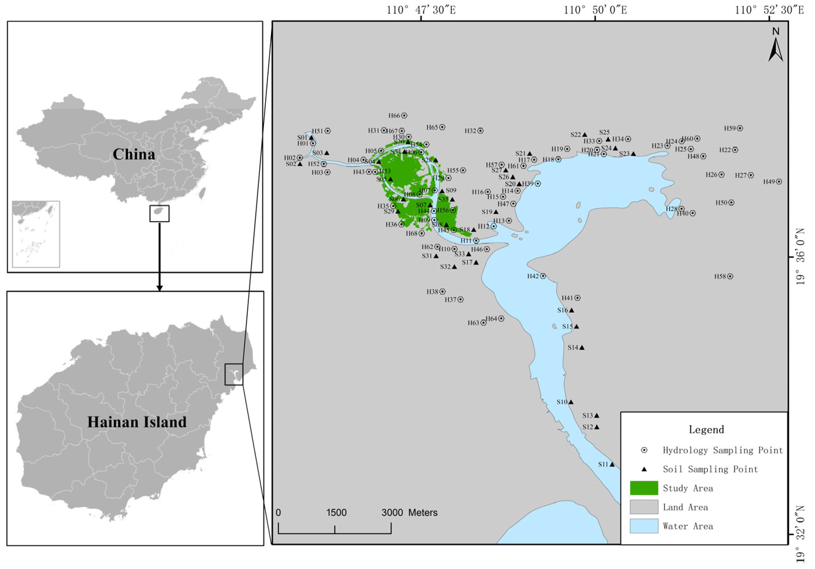
2. Study Site
3. Materials and Methods
3.1. Data Collection and Processing
- (1)
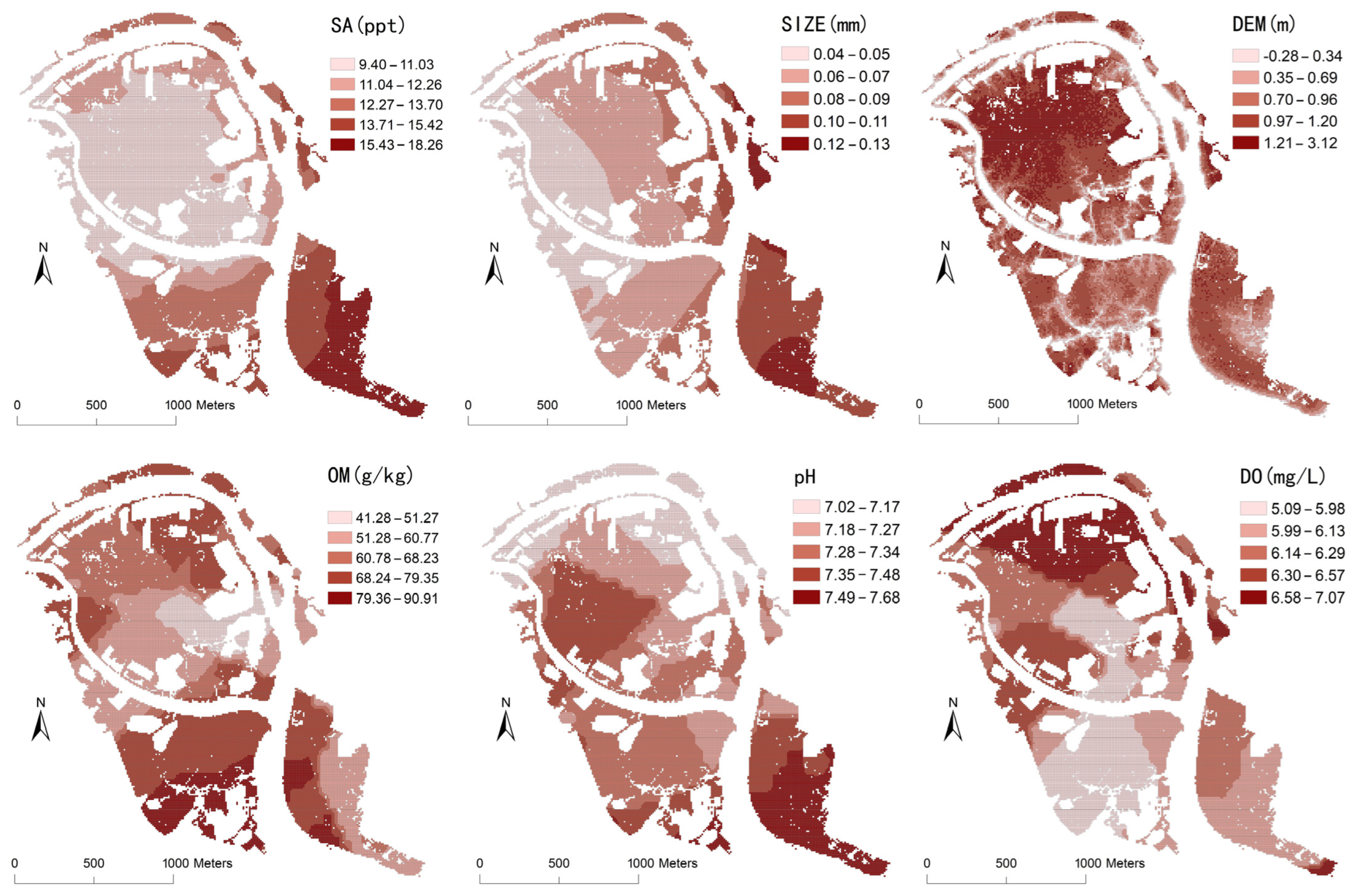
- Soil and water environment data. Soil factors included organic matter, total nitrogen, total phosphorus, total potassium, and particle size, while water environment factors included pH, salinity, and dissolved oxygen. Field sampling of 67 soil sites and 79 water sites was completed in the Bamwan Area from 2021 to 2022 (Figure 1). The pH, salinity, and dissolved oxygen of water were determined on-site, and the soil organic matter, total nitrogen, total phosphorus, total potassium, and particle size were measured using the potassium dichromate volumetric method, Kjeldahl method, alkali melt-molybdenum-antimony resistance spectrophotometry, atomic absorption spectrophotometry, and laser particle size analyzer, respectively.
- (2)
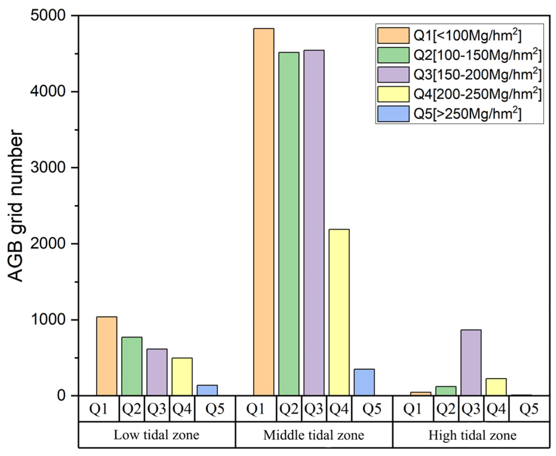
- Tidal data. Based on the average tidal data of Qinglan Port from 2000 to 2019, the neap low water line, spring low water line, neap high water line, and spring high water line were determined. The intertidal zones in the study area were then extracted: low water zone (−0.15 m to 0.55 m), mid-tide zone (0.55 m to 1.33 m), and high water zone (1.33 m to 2.12 m).
- (3)
- Mangrove plant species. The mangrove plant species in the study area were primarily divided into five species and one genera: B. sexangula (BS), E. agallocha (EA), R. apiculata (RA), H. tiliaceus (HT), and L. racemosa (LR), Sonneratia spp. (SS, including S. alba, S. apetala, and S. ovata). UAV ortho imagery with 0.06 m spatial resolution was used, and supervised classification was performed using the support vector machine, minimum distance method, and maximum likelihood method. The results from the maximum likelihood method that had the highest classification accuracy and Kappa coefficient were selected. These results were then combined with field investigation data, UAV aerial photography, and historical data to manually refine the supervised classification results, resulting in the spatial distribution map of mangrove plants in the study area (Figure 2), with a modified classification accuracy of about 87% (Table 1).
- (4)
- UAV Orthophoto Image Acquisition and Preprocessing. The orthophoto images were acquired in the field using a DJI Phantom 4 quadcopter UAV (SZ DJI Technology Co., Ltd., Shenzhen, Guangdong Province, China) equipped with a camera system. The camera system included six 1/2.9-inch CMOS (Complementary Metal-Oxide-Semiconductor) sensors, with one color sensor for visible light imaging and five monochromatic sensors for multispectral imaging (2.08 million effective pixels). The monochromatic sensors covered five multispectral imaging bands: blue (450 nm), green (560 nm), red (650 nm), red-edge (730 nm), and near-infrared (840 nm). To ensure the quality of the images and to successfully capture comprehensive mangrove vegetation data, aerial photography was conducted during low tide and under sufficient sunlight. The DJI DJIGO software system (DJI Go v3.1.72(799_go3_official)) was used for flight path planning, setting the sensor’s shooting angle to 90° vertical to the ground, with a 70% lateral overlap and a 60% longitudinal overlap, flying at a speed of 3 m/s and an altitude of 100 m. A 90% forward overlap and 70% side overlap were used. Before each flight mission, a whiteboard was used for radiometric calibration of the sensors, resulting in images with a resolution of 0.1 m. The images were processed by loading the original UAV POS (position and orientation system) data and image data using free network matching; feature point coordinates were extracted from the point cloud; the extracted feature points were imported and underwent bundle adjustment in the software; and after satisfactory adjustment, DSM/DEM production was carried out, and the final orthomosaic image was produced.
- (5)
- UAV-LiDAR Data Acquisition and Preprocessing. The LiDAR data in the study area were collected using a Hornet quadcopter UAV equipped with a Huace AS900 multiplatform LiDAR scanning system (sensor: RIEGL-VUX-1UVA) (Shanghai Huace Navigation Technology Ltd., Shanghai, China). The AS-900HL LiDAR system’s multiple return wave technology allowed it to penetrate vegetation, quickly obtaining high-precision laser point clouds under complex terrain conditions. The point cloud data collected had a density of ≥100 points/m2, with a median error in plane accuracy of ≤0.1 m and a median error in elevation accuracy of ≤0.15 m. Before the UAV flight, tidal data for the study area were collected, and actual data collection was conducted during low tide. The flight was conducted at an altitude of 150 m, at a speed of 7 m/s, with a 70% lateral overlap and an 80% forward overlap, following a snake-shaped flight path.
- (6)
- Biomass data. The AGB and the density of each quadrat were estimated based on 116 quadrat data collected from June to August in 2022 and 2023 and known mangrove AGB allometry equations. The data were split into a 7:3 ratio for the training set and validation set. Using a two-order model, mangrove height and canopy were first extracted by LiDAR. Then, the tree height and canopy of the full coverage area of the study were retrieved using spectral characteristic variables, polarization characteristic variables, and texture information from Sentinel-2 and Landsat. Finally, tree height, canopy, and image spectral characteristics were combined. The inverse model of mangrove AGB was constructed using a random forest regression algorithm. The optimal inversion results have an R2 of 0.68 and an RMSE of 43.375, indicating good accuracy (Figure 3). Applying the optimal model to the entire study area, the mangrove AGB map for the whole area was obtained.
3.2. Research Method
3.2.1. Spatial Statistical Analysis
- (1)
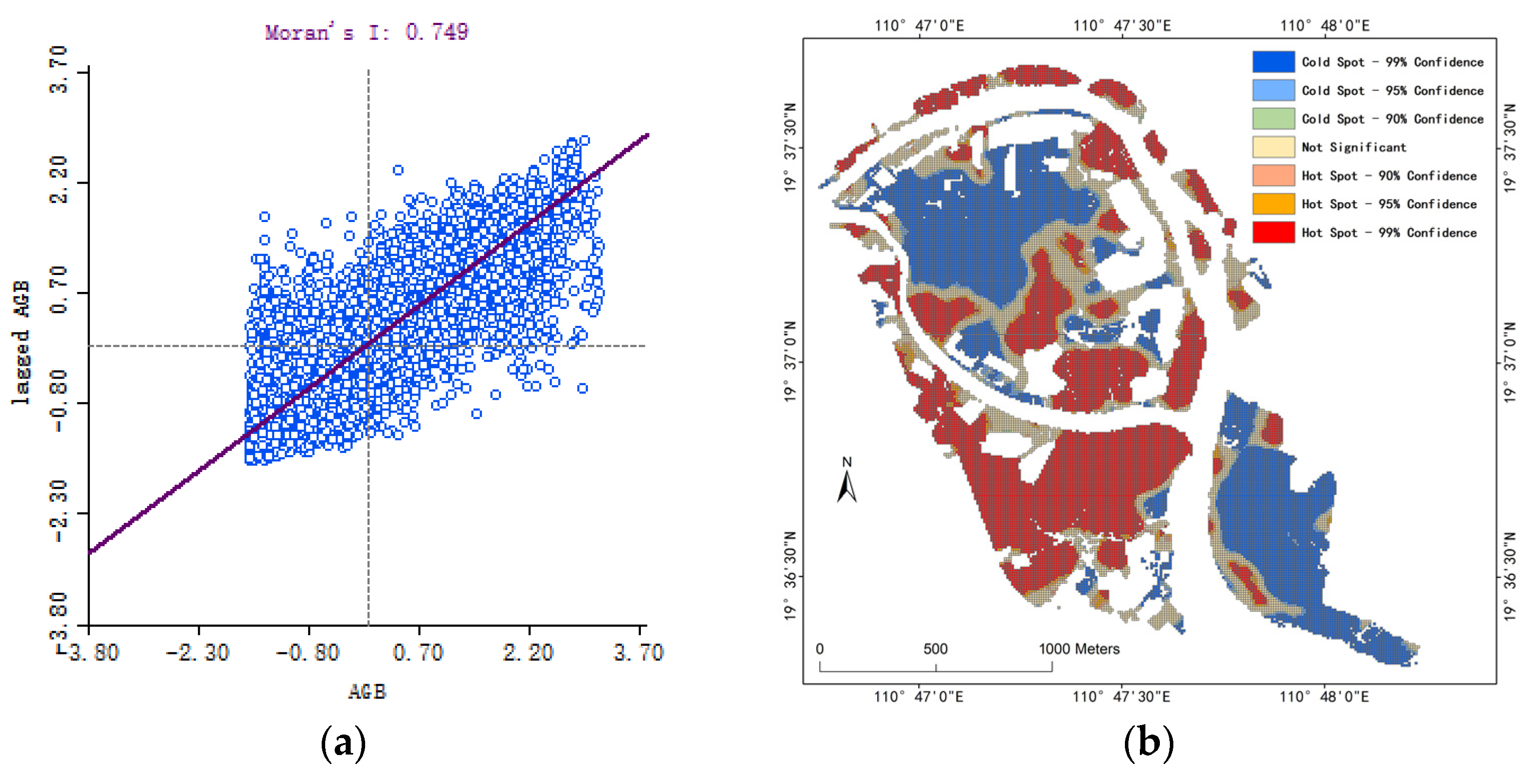
- Moran’s I: The global Moran’s I coefficient was used to describe the overall correlation degree of regions and to reflect the overall spatial agglomeration characteristics. The calculation formula is as follows [44]:where I is the global autocorrelation index; and are the index values of attribute unit and are the mean values; and is a spatial weight matrix, which reveals the spatial differentiation of mangrove AGB. Moran’s I ∈ [−1, 1], where I < 0 indicates that there is a spatial negative correlation between the observed values, and I > 0 indicates a spatial positive correlation.
- (2)
- Getis-Ord Gi*: The ArcGIS Getis-ORD Gi* analysis tool was used to identify the hotspots and coldspots of mangrove AGB in the study area. The hotspots or coldspots represent the spatial agglomeration of high or low AGB values. The calculation formula is as follows [45]:where Gi∗ denotes the Z value (z-score). A positive Z value indicates a hotspot (high-value aggregation), with larger values signifying stronger hotspots. Conversely, a negative Z value indicates a coldspot (low-value aggregation), with smaller values indicating stronger coldspots.
3.2.2. Geographic Detector
3.2.3. Regression Analysis
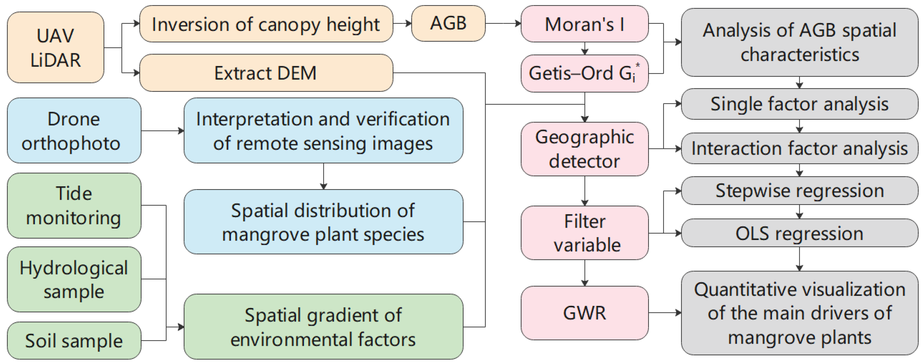
3.3. Technical Overview
4. Results
4.1. Descriptive Statistical Analysis of Mangrove AGB and Various Environmental Factors
4.2. Spatial Distribution Characteristics of Mangrove AGB
4.2.1. AGB Spatial Autocorrelation
4.2.2. AGB Hotspot Analysis
4.3. Coupling Analysis of Spatial Differentiation of AGB and Influence Factors
4.4. Screening of Driving Factors for Mangrove AGB Spatial Differentiation
5. Discussion
5.1. Comparative Analysis of AGB Distribution Pattens and Drivers
5.2. The Main Driving Factors of Mangrove AGB Spatial Heterogeneity
5.3. Comparison and Limitation of Analysis Methods of Influencing Factors
6. Conclusions
- (1)
- The spatial analysis of mangrove AGB revealed significant local clustering, with “high–high” hotspots mainly in the southwest and northeast and “low–low” coldspots in the central and southeastern regions, identifying key areas for potential mangrove quality improvement.
- (2)
- CLA, pH, TK, SA, DO, DEM, OM, TP, and TK emerged as the primary factors influencing the spatial differentiation of mangrove AGB. Interaction effects significantly enhanced the explanatory power of each factor, revealing both synergistic interactions and nonlinear enhancements among them. This underscores that the impact of various factors on mangrove AGB involves complex interactions beyond simple positive or negative correlations among individual factors.
- (3)
- The main drivers of mangrove AGB spatial differentiation were identified through comprehensive analysis using geographic detectors and multiple regression models, considering single-factor effects, two-factor interactions, and multiple factors. Factors were ranked by their influence intensity from highest to lowest: TN > TK > DEM > DO > OM > pH. TN exhibited the strongest effect on AGB (0.832), followed by TK, while pH had the least effect. TK, TN, OM, pH, and DO were positively correlated with mangrove AGB, promoting its growth. Conversely, DEM exhibited a negative correlation with AGB, indicating an inhibitory effect.
Author Contributions
Funding
Institutional Review Board Statement
Informed Consent Statement
Data Availability Statement
Acknowledgments
Conflicts of Interest
References
- Komiyama, A.; Ong, J.E.; Poungparn, S. Allometry, biomass, and productivity of mangrove forests: A review. Aquat. Bot. 2008, 89, 128–137. [Google Scholar] [CrossRef]
- Hickey, S.; Callow, N.; Phinn, S.; Lovelock, C.; Duarte, C.M. Spatial complexities in aboveground carbon stocks of a semi-arid mangrove community: A remote sensing height-biomass-carbon approach. Estuar. Coast. Shelf Sci. 2018, 200, 194–201. [Google Scholar] [CrossRef]
- Kauffman, J.B.; Adame, M.F.; Arifanti, V.B.; Schile-Beers, L.M.; Bernardino, A.F.; Bhomia, R.K.; Donato, D.C.; Feller, I.C.; Ferreira, T.O.; Garcia, M.d.C.J. Total ecosystem carbon stocks of mangroves across broad global environmental and physical gradients. Ecol. Monogr. 2020, 90, e01405. [Google Scholar] [CrossRef]
- Wang, F.; Sanders, C.J.; Santos, I.R.; Tang, J.; Schuerch, M.; Kirwan, M.L.; Kopp, R.E.; Zhu, K.; Li, X.; Yuan, J. Global blue carbon accumulation in tidal wetlands increases with climate change. Natl. Sci. Rev. 2021, 8, nwaa296. [Google Scholar] [CrossRef] [PubMed]
- Fu, C.; Li, Y.; Zeng, L.; Tu, C.; Wang, X.; Ma, H.; Xiao, L.; Christie, P.; Luo, Y. Climate and mineral accretion as drivers of mineral-associated and particulate organic matter accumulation in tidal wetland soils. Glob. Chang. Biol. 2024, 30, e17070. [Google Scholar] [CrossRef]
- Ovington, J.D. The form, weights and productivity of tree species grown in close stands. New Phytol. 1956, 55, 289–304. [Google Scholar] [CrossRef]
- Rajkaran, A.; Adams, J.B.; du Preez, D.R. A method for monitoring mangrove harvesting at the Mngazana estuary, South Africa. Afr. J. Aquat. Sci. 2004, 29, 57–65. [Google Scholar] [CrossRef]
- Abdul-Hamid, H.; Mohamad-Ismail, F.-N.; Mohamed, J.; Samdin, Z.; Abiri, R.; Tuan-Ibrahim, T.-M.; Mohammad, L.-S.; Jalil, A.-M.; Naji, H.-R. Allometric equation for aboveground biomass estimation of mixed mature mangrove forest. Forests 2022, 13, 325. [Google Scholar] [CrossRef]
- Datta, D.; Dey, M.; Ghosh, P.K.; Pal, A.P. Development of a spatially explicit model of blue carbon storages in tropical mudflat environment through integrated radar-optical approach and ground-based measurements. Ecol. Inform. 2024, 80, 102509. [Google Scholar] [CrossRef]
- Rahman, M.S.; Donoghue, D.N.; Bracken, L.J.; Mahmood, H. Biomass estimation in mangrove forests: A comparison of allometric models incorporating species and structural information. Environ. Res. Lett. 2021, 16, 124002. [Google Scholar] [CrossRef]
- Allen, M.J.; Grieve, S.W.; Owen, H.J.; Lines, E.R. Tree species classification from complex laser scanning data in Mediterranean forests using deep learning. Methods Ecol. Evol. 2023, 14, 1657–1667. [Google Scholar] [CrossRef]
- Fan, G.; Nan, L.; Chen, F.; Dong, Y.; Wang, Z.; Li, H.; Chen, D. A new quantitative approach to tree attributes estimation based on LiDAR point clouds. Remote Sens. 2020, 12, 1779. [Google Scholar] [CrossRef]
- Weiser, H.; Schäfer, J.; Winiwarter, L.; Krašovec, N.; Fassnacht, F.E.; Höfle, B. Individual tree point clouds and tree measurements from multi-platform laser scanning in German forests. Earth Syst. Sci. Data 2022, 14, 2989–3012. [Google Scholar] [CrossRef]
- Stovall, A.E.; Vorster, A.G.; Anderson, R.S.; Evangelista, P.H.; Shugart, H.H. Non-destructive aboveground biomass estimation of coniferous trees using terrestrial LiDAR. Remote Sens. Environ. 2017, 200, 31–42. [Google Scholar] [CrossRef]
- Hemati, M.; Mahdianpari, M.; Shiri, H.; Mohammadimanesh, F. Integrating SAR and optical data for aboveground biomass estimation of coastal wetlands using machine learning: Multi-scale approach. Remote Sens. 2024, 16, 831. [Google Scholar] [CrossRef]
- Tian, Y.; Huang, H.; Zhou, G.; Zhang, Q.; Tao, J.; Zhang, Y.; Lin, J. Aboveground mangrove biomass estimation in Beibu Gulf using machine learning and UAV remote sensing. Sci. Total. Environ. 2021, 781, 146816. [Google Scholar] [CrossRef]
- Kaimuddin, M.I.; Kusmana, C.; Setiawan, Y. Vegetation structure, biomass, and carbon of Mangrove Forests in Ambon Bay, Maluku, Indonesia. J. Pengelolaan Sumberd. Alam Dan Lingkung. (J. Nat. Resour. Environ. Manag.) 2023, 13, 710–722. [Google Scholar] [CrossRef]
- Pham, T.D.; Yokoya, N.; Xia, J.; Ha, N.T.; Le, N.N.; Nguyen, T.T.T.; Dao, T.H.; Vu, T.T.P.; Pham, T.D.; Takeuchi, W. Comparison of machine learning methods for estimating mangrove above-ground biomass using multiple source remote sensing data in the red river delta biosphere reserve, Vietnam. Remote Sens. 2020, 12, 1334. [Google Scholar] [CrossRef]
- Uddin, M.M.; Abdul Aziz, A.; Lovelock, C.E. Importance of mangrove plantations for climate change mitigation in Bangladesh. Glob. Chang. Biol. 2023, 29, 3331–3346. [Google Scholar] [CrossRef]
- Campbell, A.D.; Fatoyinbo, T.; Charles, S.P.; Bourgeau-Chavez, L.L.; Goes, J.; Gomes, H.; Halabisky, M.; Holmquist, J.; Lohrenz, S.; Mitchell, C. A review of carbon monitoring in wet carbon systems using remote sensing. Environ. Res. Lett. 2022, 17, 025009. [Google Scholar] [CrossRef]
- Li, S.; Zhu, Z.; Deng, W.; Zhu, Q.; Xu, Z.; Peng, B.; Guo, F.; Zhang, Y.; Yang, Z. Estimation of aboveground biomass of different vegetation types in mangrove forests based on UAV remote sensing. Sustain. Horiz. 2024, 11, 100100. [Google Scholar] [CrossRef]
- Salum, R.B.; Robinson, S.A.; Rogers, K. A validated and accurate method for quantifying and extrapolating mangrove above-ground biomass using LiDAR data. Remote Sens. 2021, 13, 2763. [Google Scholar] [CrossRef]
- Simard, M.; Fatoyinbo, L.; Smetanka, C.; Rivera-Monroy, V.H.; Castañeda-Moya, E.; Thomas, N.; Van der Stocken, T. Mangrove canopy height globally related to precipitation, temperature and cyclone frequency. Nat. Geosci. 2019, 12, 40–45. [Google Scholar] [CrossRef]
- Rijal, S.S.; Pham, T.D.; Noer’Aulia, S.; Putera, M.I.; Saintilan, N. Mapping mangrove above-ground carbon using multi-source remote sensing data and machine learning approach in Loh Buaya, Komodo National Park, Indonesia. Forests 2023, 14, 94. [Google Scholar] [CrossRef]
- Lugo, A.E. Mangrove ecosystems: Successional or steady state? Biotropica 1980, 12, 65–72. [Google Scholar] [CrossRef]
- Pillodar, F.; Suson, P.; Aguilos, M.; Amparado, R., Jr. Mangrove Resource Mapping Using Remote Sensing in the Philippines: A Systematic Review and Meta-Analysis. Forests 2023, 14, 1080. [Google Scholar] [CrossRef]
- Mafi-Gholami, D.; Jaafari, A.; Zenner, E.K.; Kamari, A.N.; Bui, D.T. Spatial modeling of exposure of mangrove ecosystems to multiple environmental hazards. Sci. Total. Environ. 2020, 740, 140167. [Google Scholar] [CrossRef] [PubMed]
- Velázquez-Pérez, C.; Romero-Berny, E.I.; Miceli-Méndez, C.L.; Moreno-Casasola, P.; López, S. Geoforms and Biogeography Defining Mangrove Primary Productivity: A Meta-Analysis for the American Pacific. Forests 2024, 15, 1215. [Google Scholar] [CrossRef]
- Berger, U.; Hildenbrandt, H. A new approach to spatially explicit modelling of forest dynamics: Spacing, ageing and neighbourhood competition of mangrove trees. Ecol. Model. 2000, 132, 287–302. [Google Scholar] [CrossRef]
- Crase, B.; Liedloff, A.; Vesk, P.A.; Burgman, M.A.; Wintle, B.A. Hydroperiod is the main driver of the spatial pattern of dominance in mangrove communities. Glob. Ecol. Biogeogr. 2013, 22, 806–817. [Google Scholar] [CrossRef]
- Hwang, Y.-H.; Chen, S.-C. Effects of ammonium, phosphate, and salinity on growth, gas exchange characteristics, and ionic contents of seedlings of mangrove Kandelia candel (L.) Druce. Bot. Bull. Acad. Sin. 2001, 42, 5–7. [Google Scholar] [CrossRef]
- Sasmito, S.D.; Kuzyakov, Y.; Lubis, A.A.; Murdiyarso, D.; Hutley, L.B.; Bachri, S.; Friess, D.A.; Martius, C.; Borchard, N. Organic carbon burial and sources in soils of coastal mudflat and mangrove ecosystems. CATENA 2020, 187, 104414. [Google Scholar] [CrossRef]
- Cai, C.; Anton, A.; Duarte, C.M.; Agusti, S. Environment. Spatial variations in element concentrations in Saudi Arabian Red Sea Mangrove and Seagrass ecosystems: A comparative analysis for bioindicator selection. Earth Syst. Environ. 2024, 8, 395–415. [Google Scholar] [CrossRef]
- Xu, C.; Hu, G.; Zhang, Z.; Zhong, C. Ecological Stoichiometric Characteristics of the Mangrove Ecosystem in Beibu Gulf, China. Appl. Ecol. Environ. Res. 2024, 22, 1971–1981. [Google Scholar] [CrossRef]
- Grindrod, J. Holocene sea level history of a toropical estuary: Missionary Bay, North Queensland. Quat. Sci. Rev. 1984, 30, 151–178. [Google Scholar] [CrossRef]
- Smith III, T.J.; Boto, K.G.; Frusher, S.D.; Giddins, R.L. Keystone species and mangrove forest dynamics: The influence of burrowing by crabs on soil nutrient status and forest productivity. Estuar. Coast. Shelf Sci. 1991, 33, 419–432. [Google Scholar] [CrossRef]
- Azman, M.S.; Sharma, S.; Shaharudin, M.A.M.; Hamzah, M.L.; Adibah, S.N.; Zakaria, R.M.; MacKenzie, R.A. Stand structure, biomass and dynamics of naturally regenerated and restored mangroves in Malaysia. For. Ecol. Manag. 2021, 482, 118852. [Google Scholar] [CrossRef]
- Martinez del Castillo, E.; Zang, C.S.; Buras, A.; Hacket-Pain, A.; Esper, J.; Serrano-Notivoli, R.; Hartl, C.; Weigel, R.; Klesse, S.; Resco de Dios, V. Climate-change-driven growth decline of European beech forests. Commun. Biol. 2022, 5, 163. [Google Scholar] [CrossRef]
- Chowdhury, A.; Naz, A.; Maiti, S.K. Community-based, cost-effective multispecies mangrove restoration innovation to maximize soil blue carbon pool and humic acid and fulvic acid concentrations at Indian Sundarbans. Environ. Sci. Pollut. Res. 2024, 1–14. [Google Scholar] [CrossRef]
- Azeez, A.; Gnanappazham, L.; Muraleedharan, K.; Revichandran, C.; John, S.; Seena, G.; Thomas, J. Multi-decadal changes of mangrove forest and its response to the tidal dynamics of thane creek, Mumbai. J. Sea Res. 2022, 180, 102162. [Google Scholar] [CrossRef]
- Long, C.; Dai, Z.; Wang, R.; Lou, Y.; Zhou, X.; Li, S.; Nie, Y. Dynamic changes in mangroves of the largest delta in northern Beibu Gulf, China: Reasons and causes. For. Ecol. Manag. 2022, 504, 119855. [Google Scholar] [CrossRef]
- Nie, X.; Jin, X.; Wu, J.; Li, W.; Wang, H.; Yao, Y. Evaluation of coastal wetland ecosystem services based on modified choice experimental model: A case study of mangrove wetland in Beibu Gulf, Guangxi. Habitat Int. 2023, 131, 102735. [Google Scholar] [CrossRef]
- Joshi, H.G.; Ghose, M. Community structure, species diversity, and aboveground biomass of the Sundarbans mangrove swamps. Trop. Ecol. 2014, 283–303. [Google Scholar]
- Xu, H.; Zhang, C. Development and applications of GIS-based spatial analysis in environmental geochemistry in the big data era. Environ. Geochem. Health 2023, 45, 1079–1090. [Google Scholar] [CrossRef] [PubMed]
- Feng, Y.; Chen, X.; Gao, F.; Liu, Y. Impacts of changing scale on Getis-Ord Gi* hotspots of CPUE: A case study of the neon flying squid (Ommastrephes bartramii) in the northwest Pacific Ocean. Acta Oceanol. Sin. 2018, 37, 67–76. [Google Scholar] [CrossRef]
- Beale, C.M.; Lennon, J.J.; Yearsley, J.M.; Brewer, M.J.; Elston, D.A. Regression analysis of spatial data. Ecol. Lett. 2010, 13, 246–264. [Google Scholar] [CrossRef]
- Chang, Y.; Liao, J.; Zhang, L. Temporal and spatial variations of mangroves and their driving factors in Southeast Asia. Trop. Geogr. 2023, 43, 31–42. [Google Scholar] [CrossRef]
- Wang, J.; Sun, Q.; Zou, L. Spatial-temporal evolution and driving mechanism of rural production-living-ecological space in Pingtan islands, China. Habitat Int. 2023, 137, 102833. [Google Scholar] [CrossRef]
- Song, Y.; Wang, J.; Ge, Y.; Xu, C. An optimal parameters-based geographical detector model enhances geographic characteristics of explanatory variables for spatial heterogeneity analysis: Cases with different types of spatial data. GISci. Remote Sens. 2020, 57, 593–610. [Google Scholar] [CrossRef]
- Cohen, A. Dummy variables in stepwise regression. Am. Stat. 1991, 45, 226–228. [Google Scholar] [CrossRef]
- Burton, A.L. OLS (Linear) regression. Encycl. Res. Methods Criminol. Crim. Justice 2021, 2, 509–514. [Google Scholar] [CrossRef]
- McMillen, D.P. Geographically weighted regression: The analysis of spatially varying relationships. Geogr. Anal. 2004, 35, 272–275. [Google Scholar] [CrossRef]
- Brunsdon, C.; Fotheringham, S.; Charlton, M. Geographically weighted regression. J. R. Stat. Soc. Ser. D 1998, 47, 431–443. [Google Scholar] [CrossRef]
- Murphy, B. Key soil functional properties affected by soil organic matter-evidence from published literature. In Proceedings of the IOP Conference Series: Earth and Environmental Science, Bendigo, VIC, Australia, 24–27 March 2014; p. 012008. [Google Scholar]
- Cahoon, D.R. Measuring and Interpreting the Surface and Shallow Subsurface Process Influences on Coastal Wetland Elevation: A Review. Estuaries Coasts 2024, 47, 1708–1734. [Google Scholar] [CrossRef]
- Meiling, L. Relationship between Mangrove Distribution and Soil Characters at Dongzhai Harbor and Qinglan Harbor, Hainan. Revel. Sci. Issue Plant Sci. 2008, 56, 25–38. [Google Scholar]
- Mattone, C.; Sheaves, M. Patterns, drivers and implications of dissolved oxygen dynamics in tropical mangrove forests. Estuar. Coast. Shelf Sci. 2017, 197, 205–213. [Google Scholar] [CrossRef]
- Jiao, M.; Zhou, W.; Long, C.; Zhang, L.; Xu, P.; Li, H.; Suo, A.; Yue, W.J. Dietary reconstruction and influencing factors of oysters cultured in a typical estuarine bay of South China. J. Clean. Prod. 2024, 449, 141773. [Google Scholar] [CrossRef]
- Zaman, M.R.; Rahman, M.S.; Ahmed, S.; Zuidema, P. What drives carbon stocks in a mangrove forest? The role of stand structure, species diversity and functional traits. Estuar. Coast. Shelf Sci. 2023, 295, 108556. [Google Scholar] [CrossRef]
- Zhao, C.; Jia, M.; Zhang, R.; Wang, Z.; Ren, C.; Mao, D.; Wang, Y. Mangrove species mapping in coastal China using synthesized Sentinel-2 high-separability images. Remote Sens. Environ. 2024, 307, 114151. [Google Scholar] [CrossRef]
- Brown, C.; Sjögersten, S.; Ledger, M.J.; Parish, F.; Boyd, D. Remote Sensing for Restoration Change Monitoring in Tropical Peat Swamp Forests in Malaysia. Remote Sens. 2024, 16, 2690. [Google Scholar] [CrossRef]
- Wang, R.; Sun, Y.; Zong, J.; Wang, Y.; Cao, X.; Wang, Y.; Cheng, X.; Zhang, W. Remote Sensing Application in Ecological Restoration Monitoring: A Systematic Review. Remote Sens. 2024, 16, 2204. [Google Scholar] [CrossRef]
- Meng, Y.; Bai, J.; Gou, R.; Cui, X.; Feng, J.; Dai, Z.; Diao, X.; Zhu, X.; Lin, G. Relationships between above-and below-ground carbon stocks in mangrove forests facilitate better estimation of total mangrove blue carbon. Carbon Balance Manag. 2021, 16, 8. [Google Scholar] [CrossRef] [PubMed]
- Sharma, S.; Ray, R.; Martius, C.; Murdiyarso, D. Carbon stocks and fluxes in Asia-Pacific mangroves: Current knowledge and gaps. Environ. Res. Lett. 2023, 18, 044002. [Google Scholar] [CrossRef]
- Bai, J.; Meng, Y.; Gou, R.; Lyu, J.; Dai, Z.; Diao, X.; Zhang, H.; Luo, Y.; Zhu, X.; Lin, G. Mangrove diversity enhances plant biomass production and carbon storage in Hainan island, China. Funct. Ecol. 2021, 35, 774–786. [Google Scholar] [CrossRef]
- Cooray, P.L.I.G.M.; Kodikara, K.A.S.; Kumara, M.P.; Jayasinghe, U.I.; Madarasinghe, S.K.; Dahdouh-Guebas, F.; Gorman, D.; Huxham, M.; Jayatissa, L.P. Climate and intertidal zonation drive variability in the carbon stocks of Sri Lankan mangrove forests. Geoderma 2021, 389, 114929. [Google Scholar] [CrossRef]
- Meng, Y.; Gou, R.; Bai, J.; Moreno-Mateos, D.; Davis, C.C.; Wan, L.; Song, S.; Zhang, H.; Zhu, X.; Lin, G.; et al. Spatial patterns and driving factors of carbon stocks in mangrove forests on Hainan Island, China. Glob. Ecol. Biogeogr. 2022, 31, 1692–1706. [Google Scholar] [CrossRef]
- Djamaluddin, R.; Holmes, R.; Djabar, B. Assessing species composition and structural attributes across different habitats to evaluate changes and management effectiveness of protected mangroves. For. Ecol. Manag. 2024, 561, 121857. [Google Scholar] [CrossRef]
- You, Q.; Deng, W.; Tang, X.; Liu, Y.; Lei, P.; Chen, J.; You, H. Monitoring of mangrove dynamic change in Beibu Gulf of Guangxi based on reconstructed time series images. Sci. Total. Environ. 2024, 917, 170395. [Google Scholar] [CrossRef] [PubMed]
- Naidoo, G. Differential effects of nitrogen and phosphorus enrichment on growth of dwarf Avicennia marina mangroves. Aquat. Bot. 2009, 90, 184–190. [Google Scholar] [CrossRef]
- Reef, R.; Feller, I.C.; Lovelock, C.E. Nutrition of mangroves. Tree Physiol. 2010, 30, 1148–1160. [Google Scholar] [CrossRef]
- Sardans, J.; Rivas-Ubach, A.; Peñuelas, J. The C: N: P stoichiometry of organisms and ecosystems in a changing world: A review and perspectives. Perspect. Plant Ecol. Evol. Syst. 2012, 14, 33–47. [Google Scholar] [CrossRef]
- Wang, R.; Bicharanloo, B.; Hou, E.; Jiang, Y.; Dijkstra, F.A. Phosphorus supply increases nitrogen transformation rates and retention in soil: A global meta-analysis. Earth’s Futur. 2022, 10, e2021EF002479. [Google Scholar] [CrossRef]
- Sun, X.; Bao, D.; Li, H.; Zhao, R.; Li, J.; Yu, J.; Su, J. Plant stoichiometric hierarchical responses to nutrient enrichment can enhance understanding regarding the process of biodiversity loss. Ecol. Eng. 2024, 200, 107173. [Google Scholar] [CrossRef]
- Adame, M.; Reef, R.; Santini, N.; Najera, E.; Turschwell, M.; Hayes, M.; Masque, P.; Lovelock, C. Mangroves in arid regions: Ecology, threats, and opportunities. Estuar. Coast. Shelf Sci. 2021, 248, 106796. [Google Scholar] [CrossRef]
- Sherman, R.E.; Fahey, T.J.; Martinez, P. Spatial patterns of biomass and aboveground net primary productivity in a mangrove ecosystem in the Dominican Republic. Ecosystems 2003, 6, 384–398. [Google Scholar] [CrossRef]
- Burchett, M.; Field, C.; Pulkownik, A. Salinity, growth and root respiration in the grey mangrove, Avicennia marina. Physiol. Plant. 1984, 60, 113–118. [Google Scholar] [CrossRef]
- Fatoyinbo, T.; Washington-Allen, R.; Simard, M.; Shugart, H. Landscape Scale Height, Biomass and Carbon Estimation of Mangrove Forests with SRTM Elevation Data. In Proceedings of the AGU Fall Meeting Abstracts, San Francisco, CA, USA, 11–15 December 2006; p. B44B–02. [Google Scholar]
- Chaikaew, P.; Chavanich, S. Spatial variability and relationship of mangrove soil organic matter to organic carbon. Appl. Environ. Soil Sci. 2017, 2017, 4010381. [Google Scholar] [CrossRef]
- Sakeri, F.; Tajudin, N.S.M.; Shahari, R. Evaluation of Sediment Quality along the River of Balok Mangrove Forest, Kuantan, Pahang, Malaysia. Revel. Sci. 2023, 1, 52–57. [Google Scholar]


| Species | Classification Result | |||||||
|---|---|---|---|---|---|---|---|---|
| BS | EA | HT | LR | RA | SS | Total | Producer’s Accuracy | |
| BS | 162 | 1 | 5 | 9 | 2 | 6 | 185 | 87.57% |
| EA | 2 | 103 | 3 | 5 | 6 | 4 | 123 | 83.74% |
| HT | 1 | 2 | 92 | 2 | 4 | 5 | 106 | 86.79% |
| LR | 9 | 5 | 6 | 225 | 4 | 6 | 255 | 88.24% |
| RA | 3 | 6 | 4 | 2 | 92 | 1 | 108 | 85.19% |
| SS | 5 | 4 | 3 | 2 | 1 | 105 | 120 | 87.50% |
| Total | 182 | 121 | 113 | 245 | 109 | 127 | 897 | |
| User’s Accuracy | 89.01% | 85.12% | 81.42% | 91.84% | 84.40% | 82.68% | ||
| Overall Accuracy: 86.85%; Cohen’s Kappa coefficient: 0.84 | ||||||||
| Criterion | Interaction |
|---|---|
| Nonlinear attenuation | |
| Single-factor nonlinear enhancement | |
| Two-factor enhancement | |
| Independent | |
| Nonlinear enhancement |
| Independent Variable | Abbreviation | Minimum Value | Maximum Value | Mean | Standard Deviation | Skewness | Kurtosis | Correlation Coefficient |
|---|---|---|---|---|---|---|---|---|
| Elevation | DEM | −0.28 | 3.12 | 0.93 | 0.34 | −0.68 | 0.82 | −0.229 ** |
| Salinity | SA | 9.40 | 18.26 | 12.21 | 2.01 | 0.88 | −0.16 | −0.001 |
| Water pH | PH | 7.02 | 7.68 | 7.32 | 0.13 | 0.58 | 0.59 | −0.150 ** |
| Dissolved oxygen | DO | 5.09 | 7.07 | 6.22 | 0.30 | 0.74 | −0.29 | −0.271 ** |
| Soil total nitrogen | TN | 1.62 | 2.91 | 2.25 | 0.30 | 0.09 | −0.87 | −0.230 ** |
| Soil total potassium | TK | 6.28 | 8.82 | 7.94 | 0.52 | −0.27 | −0.81 | 0.322 ** |
| Soil total phosphorus | SP | 4.25 | 26.78 | 18.37 | 5.00 | −0.68 | −0.35 | −0.151 ** |
| Soil particle size | SIZE | 0.04 | 0.13 | 0.07 | 0.02 | 0.79 | −0.65 | −0.150 ** |
| Soil organic matter | OM | 41.28 | 90.91 | 66.61 | 10.44 | 0.18 | −0.03 | 0.138 ** |
| Factor | q | Factor | q |
|---|---|---|---|
| CLA | 0.2547 ** | DEM | 0.1298 ** |
| pH | 0.2020 ** | OM | 0.1274 ** |
| TK | 0.1869 ** | SP | 0.1122 ** |
| SA | 0.1719 ** | TN | 0.1076 ** |
| DO | 0.1551 ** | SIZE | 0.0828 ** |
| Model | Unstandardized Coefficients | Standardized Coefficients | R-Squared | t | Sig. | Collinearity Statistics | ||
|---|---|---|---|---|---|---|---|---|
| B | Standard Error | Tolerance | VIF | |||||
| Constant | 195.606 | 4.980 | 0.330 | 39.278 | 0.000 | |||
| BS | 28.821 | 1.217 | 0.246 | 23.675 | 0.000 | 0.296 | 30.380 | |
| pH | −298.565 | 7.918 | −0.317 | −37.707 | 0.000 | 0.452 | 20.213 | |
| DO | −249.863 | 12.277 | −0.184 | −20.352 | 0.000 | 0.390 | 20.564 | |
| TN | −41.621 | 6.033 | −0.051 | −6.899 | 0.000 | 0.588 | 10.699 | |
| LR | −27.594 | 1.493 | −0.147 | −18.478 | 0.000 | 0.502 | 10.991 | |
| DEM | −4.612 | 3.933 | −0.008 | −1.173 | 0.041 | 0.629 | 10.589 | |
| TK | 141.802 | 9.044 | 0.142 | 15.679 | 0.000 | 0.389 | 20.572 | |
| OM | 59.991 | 5.616 | 0.065 | 10.682 | 0.000 | 0.848 | 10.180 | |
| RA | 4.020 | 1.391 | 0.024 | 2.890 | 0.004 | 0.475 | 20.105 | |
| SA | 43.404 | 7.102 | 0.055 | 6.112 | 0.000 | 0.391 | 20.555 | |
| EA | −14.737 | 1.401 | −0.103 | −10.521 | 0.000 | 0.331 | 30.026 | |
| HT | −15.424 | 1.514 | −0.087 | −10.190 | 0.000 | 0.435 | 20.297 | |
| Variable | Regression Coefficient | Standard Error | p | Variable | Regression Coefficient | Standard Error | p |
|---|---|---|---|---|---|---|---|
| BS | 28.930 | 1.227 | 0.000 | TK | 32.138 | 2.869 | 0.000 |
| pH | −85.948 | 2.567 | 0.000 | OM | 15.486 | 2.010 | 0.000 |
| DO | −61.333 | 3.375 | 0.000 | RA | 4.400 | 1.384 | 0.001 |
| TN | −13.423 | 1.788 | 0.000 | SA | 23.219 | 3.342 | 0.000 |
| LR | −27.640 | 1.509 | 0.000 | EA | −14.793 | 1.423 | 0.000 |
| DEM | −8.790 | 3.939 | 0.025 | HT | −15.168 | 1.529 | 0.000 |
| R2 | 0.337 | ||||||
| F | 753 | ||||||
| K value | 0.000 * | ||||||
| Factor | Regression Coefficient | |||
|---|---|---|---|---|
| Minimum Value | Maximum Value | Median | Mean | |
| TK | −0.391 | 0.609 | 0.218 | 0.219 |
| TN | −0.084 | 0.916 | 0.832 | 0.832 |
| OM | −0.482 | 0.518 | 0.037 | 0.038 |
| pH | −0.494 | 0.506 | 0.011 | 0.009 |
| DO | −0.466 | 0.534 | 0.067 | 0.065 |
| DEM | −0.543 | 0.457 | −0.083 | −0.085 |
Disclaimer/Publisher’s Note: The statements, opinions and data contained in all publications are solely those of the individual author(s) and contributor(s) and not of MDPI and/or the editor(s). MDPI and/or the editor(s) disclaim responsibility for any injury to people or property resulting from any ideas, methods, instructions or products referred to in the content. |
© 2024 by the authors. Licensee MDPI, Basel, Switzerland. This article is an open access article distributed under the terms and conditions of the Creative Commons Attribution (CC BY) license (https://creativecommons.org/licenses/by/4.0/).
Share and Cite
Wang, K.; Jiang, M.; Li, Y.; Kong, S.; Gao, Y.; Huang, Y.; Qiu, P.; Yang, Y.; Wan, S. Spatial Differentiation of Mangrove Aboveground Biomass and Identification of Its Main Environmental Drivers in Qinglan Harbor Mangrove Nature Reserve. Sustainability 2024, 16, 8408. https://doi.org/10.3390/su16198408
Wang K, Jiang M, Li Y, Kong S, Gao Y, Huang Y, Qiu P, Yang Y, Wan S. Spatial Differentiation of Mangrove Aboveground Biomass and Identification of Its Main Environmental Drivers in Qinglan Harbor Mangrove Nature Reserve. Sustainability. 2024; 16(19):8408. https://doi.org/10.3390/su16198408
Chicago/Turabian StyleWang, Kaiyue, Meihuijuan Jiang, Yating Li, Shengnan Kong, Yilun Gao, Yingying Huang, Penghua Qiu, Yanli Yang, and Siang Wan. 2024. "Spatial Differentiation of Mangrove Aboveground Biomass and Identification of Its Main Environmental Drivers in Qinglan Harbor Mangrove Nature Reserve" Sustainability 16, no. 19: 8408. https://doi.org/10.3390/su16198408