Article

Artificial Neural Network and Kriging Surrogate Model for Embodied Energy Optimization of Prestressed Slab Bridges

by
Lorena Yepes-Bellver
1,†,
Alejandro Brun-Izquierdo
2,†,
Julián Alcalá
3,† and
Víctor Yepes
3,*,†
1
Mechanics of Continuous Media and Theory of Structures Department, Universitat Politècnica de València, 46022 Valencia, Spain
2
School of Civil Engineering, Universitat Politècnica de València, 46022 Valencia, Spain
3
Institute of Concrete Science and Technology (ICITECH), Universitat Politècnica de València, 46022 Valencia, Spain
*
Author to whom correspondence should be addressed.
These authors contributed equally to this work.
Sustainability 2024, 16(19), 8450; https://doi.org/10.3390/su16198450 (registering DOI)
Submission received: 12 July 2024 / Revised: 31 August 2024 / Accepted: 26 September 2024 / Published: 28 September 2024

Abstract

:
The main objective of this study is to assess and contrast the efficacy of distinct spatial prediction methods in a simulation aimed at optimizing the embodied energy during the construction of prestressed slab bridge decks. A literature review and cross-sectional analysis have identified crucial design parameters that directly affect the design and construction of bridge decks. This analysis determines the critical design variables to improve the deck’s energy efficiency, providing practical guidance for engineers and professionals in the field. The methods analyzed in this study are ordinary Kriging and a multilayer perceptron neural network. The methodology involves analyzing the predictive performance of both models through error analysis and assessing their ability to identify local optima on the response surface. The results show that both models generally overestimate the observed values. The Kriging model with second-order polynomials yields a 4% relative error at the local optimum, while the neural network achieves lower root mean square errors (RMSEs). Neither the Kriging model nor the neural network provides precise predictions but point to promising solution regions. Optimizing the response surface to find a local minimum is crucial. High slenderness ratios (around 1/28) and 40 MPa concrete grade are recommended to improve energy efficiency.

1. Introduction

Construction accounts for 25% to 40% of global energy consumption [1]. The amount of energy used in constructing a structure and the associated greenhouse gas emissions are considered key indicators of its sustainability [2,3]. Therefore, interest in optimizing environmental sustainability in the construction industry has increased significantly in recent years [4,5].
Prestressed concrete offers many advantages, including longer spans that increase floor space, thinner slabs for high-rise buildings, fewer joints, and reduced maintenance costs. It offers excellent durability, crack resistance, and improved structural performance with less deformation. In addition, prestressed concrete allows for faster construction with better quality control and is ideal for repetitive structures. However, it requires high-strength materials, specialized equipment, and skilled labor, making initial construction costs higher than traditional reinforced concrete structures. Despite these disadvantages, the long-term benefits often outweigh the initial cost. Leonhart [6] provides an overview of the prestressing advantages of this technique. Warner et al. [7] offer a detailed discussion of the potential challenges of prestressed concrete.
Selecting appropriate materials and optimizing them enhances the sustainability of structures. Some studies have used energy as a critical target in this process [8,9]. Cabeza et al. [10] conducted a comprehensive review of the literature, utilizing keyword analysis to present an overview of embodied carbon and energy values. Miller et al. [11] have shown that post-tensioned concrete slabs consume less embodied energy than their reinforced concrete counterparts. However, solely reducing the structure’s weight does not guarantee a reduction in energy consumption [12].
Nevertheless, research on optimizing embodied energy in bridges still needs to be explored. Alcalá et al. [13] found that the least-cost solution only required a 5.3% increase in embodied energy consumption. In another study, Martí et al. [14] achieved energy savings of 24% for a 30 m precast bridge. Minunno et al. [15] offer a regression model and procedural guidelines for practitioners aiming to minimize the environmental impact of buildings. Furthermore, Penadés-Plà et al. [16] presented a Kriging-based optimization method for a three-span pedestrian bridge with lengths of 40-50-40 m. However, it is essential to acknowledge that research addressing energy optimization in concrete slab bridges is still scarce, indicating a clear need for more exploration.
The heuristic optimization of structures is often computationally expensive, which has led to the development of metamodels to address this challenging problem. Among the most effective methods is the Kriging predictor. This approach replaces a simulation model and provides optimal interpolation based on regression against a set of observed values from neighboring points [17]. While Kriging has yet to be widely used in the design of real structures, there are interesting examples of its application. Martínez-Frutos and Martí [18] used it to optimize the robust design of structures. They effectively decoupled the uncertainty evaluation from the optimization process. More recently, it has been employed in the optimization of structural dynamics [19], in the design of residential building typology [20], and post-tensioned bridges [21,22]. In a related study, Zhang and Wu [23] employed Kriging to establish structural vulnerability curves for RC bridges. Wu et al. [24] further applied this model to optimize finite element models of bridge structures. Cheng and Low [25] provide a new metamodel for offshore structures.
Another type of metamodel is the artificial neural network (ANN). Its structure, resembling the human brain, is formed by a network of nodes (or neurons) and connections. Thanks to their flexibility and ease of use, these networks find application in various problems, from pattern recognition to function approximation. ANNs, which are a method of machine learning, learn from training examples and provide an answer or output by the approximation of the nonlinear functions of their inputs. ANNs have been applied to predict structural behavior [26] or to support multiobjective bridge optimization [27].

2. Lightened Slab Bridge Deck Description

Hyperstatic post-tensioned concrete slabs are common on bridges ranging from 10 m to 45 m in length. With a main span of more than 50 m, this structure is not competitive and gives way to box girders. In common practice, designers typically maintain a depth/span ratio of approximately 1/25 when designing roadway slabs with three or more spans. This significant ratio ensures the slab’s structural integrity and load-bearing capacity. This solution competes with precast girders due to its structural advantages, which include higher bending and torsional stiffness, greater durability, and safety attributed to hyperstatic behavior. Nevertheless, what sets it apart is its adaptability to complex construction shapes. This unique feature simplifies the formwork and concrete pouring processes, making the design more efficient. In addition, there is no need for joints and there is greater flexibility in pile placement for improved aesthetics.
This study aims to improve the design of a prestressed, lightened slab with a specific configuration of spans: 24-34-28 m. This configuration is a standard in overpasses crossing dual-lane, dual-track highways, making the study’s findings directly applicable to real-world bridge construction. As shown in Figure 1, the slab has a constant depth and rectilinear configuration. The platform is 8.30 m wide, allowing for two lanes of 3.50 m each, 0.65 m parapets on each side, and a concrete base (see Figure 2).
This overpass is situated at kilometer 441 of the A-7 highway in Cocentaina, in the province of Alicante. Figure 3 displays an aerial image of the overpass. The bridge was designed with a depth of 1.35 m, a lower base of 4.00 m, and a span of 1.75 m, with the following dimensions: a = 0.20 m, b = 0.10 m, and d = 0.40 m. The interior lighting consisted of four circular sections with a diameter of 0.60 m. These measurements result in an internal lighting of 0.14 m3/m2 and an external lighting of 0.51 m3/m2.
Limit state theory verifies structural resistance using partial safety factors. Each design situation ensures that no ultimate and serviceability limit states are exceeded. The present study used CSiBridge v.21.0.0 software to create a three-dimensional deck model, which was subsequently analyzed and dimensioned. The assessment thoroughly examined various alternatives to identify the acting and resisting loads represented by sectional forces. These detailed force calculations align with those presented in the work of Yepes-Bellver et al. [21,22].

3. Methodology

The construction of each slab deck consumes energy. Comparing different designs involves considering various factors, such as the concrete grade, the amount of incorporated steel, the formwork surface, and the energy required for lighting. Table 1 presents the costs for different objectives, such as cost, emissions, and energy consumption [21,22].
The materials analyzed include Y-1860-S7 steel, known for its high strength and durability in structural reinforcements, and B-500-St steel, which offers good ductility and tensile strength for concrete reinforcement. Concrete types range from C-30, a medium-strength option, to C-50, an ultra-high-strength concrete. Additionally, lighting reduces structural weight to improve efficiency and cost-effectiveness, while slab formwork supports and shapes the concrete, impacting surface quality and construction speed.
Our research uses two types of predictive metamodels: Kriging and neural networks. These models are applied to 42 data points that were previously used to optimize the proposed slab bridge [21,22]. These data points, detailed in Table 2, serve a specific purpose in our research. The diversification phase uses the first 30 data points to optimize the Kriging response surface. The intensification phase uses the following 10 data points. Data number 41 represents the local optimum of the diversification phase, while number 42 is the local optimum corresponding to the intensification phase.
Once a response surface is fitted to a surrogate model, the prediction error can be measured using the root mean square error (RMSE), which will have the same units as the output values of the predictive model.
R M S E = i = 1 n y ^ i y i 2 n
where y ^ i is the estimated values, yi is the observed values, and n is the number of observations.

3.1. Kriging Metamodel

The approach involves a two-phase optimization process employing a response surface generated by a Kriging metamodel [21,22]. Latin hypercube sampling (LHS) selects uniformly distributed random numbers to analyze energy in alternatives. A Kriging model then creates and optimizes a response surface for the optimization input.
Kriging estimates an attribute’s value at a point u from a set of n values of z (Figure 4). In this context, the variable of interest is the energy required to run the board. The points from LHS sampling represent solutions. This approach predicts responses without detailed structural analysis. The “MATLAB Kriging Toolbox” Version 2.0 (DACE) is used to build a Kriging surrogate model from data pairs of inputs and responses from a computational experiment [28]. The models are deterministic, producing consistent responses for the same inputs without random error. Kriging models can be built with polynomial regressions of orders 0, 1, and 2, known as Kriging 1, Kriging 2, and Kriging 3.
Latin hypercube sampling (LHS) is a technique that selects uniformly distributed random numbers. In contrast to a simple random sample, the method offers a lower variance of the sample mean [29]. This technique entails selecting a sample at random from each interval for each variable, with the mathematical model then running repeatedly to that of the number of intervals within the probability distribution split. This process ensures the selection of initial values from each data range. LHS offers an enhanced grasp of the design space compared to that afforded by simple random sampling. It is particularly suitable for computational tests that aim to minimize systematic errors while maintaining a uniform random sample. LHS is sufficiently flexible to adapt the number of samples according to the specific requirements of the experiment. In addition, it is highly efficient in generating results within a reasonable period, thus making it a practical choice for a wide range of applications.

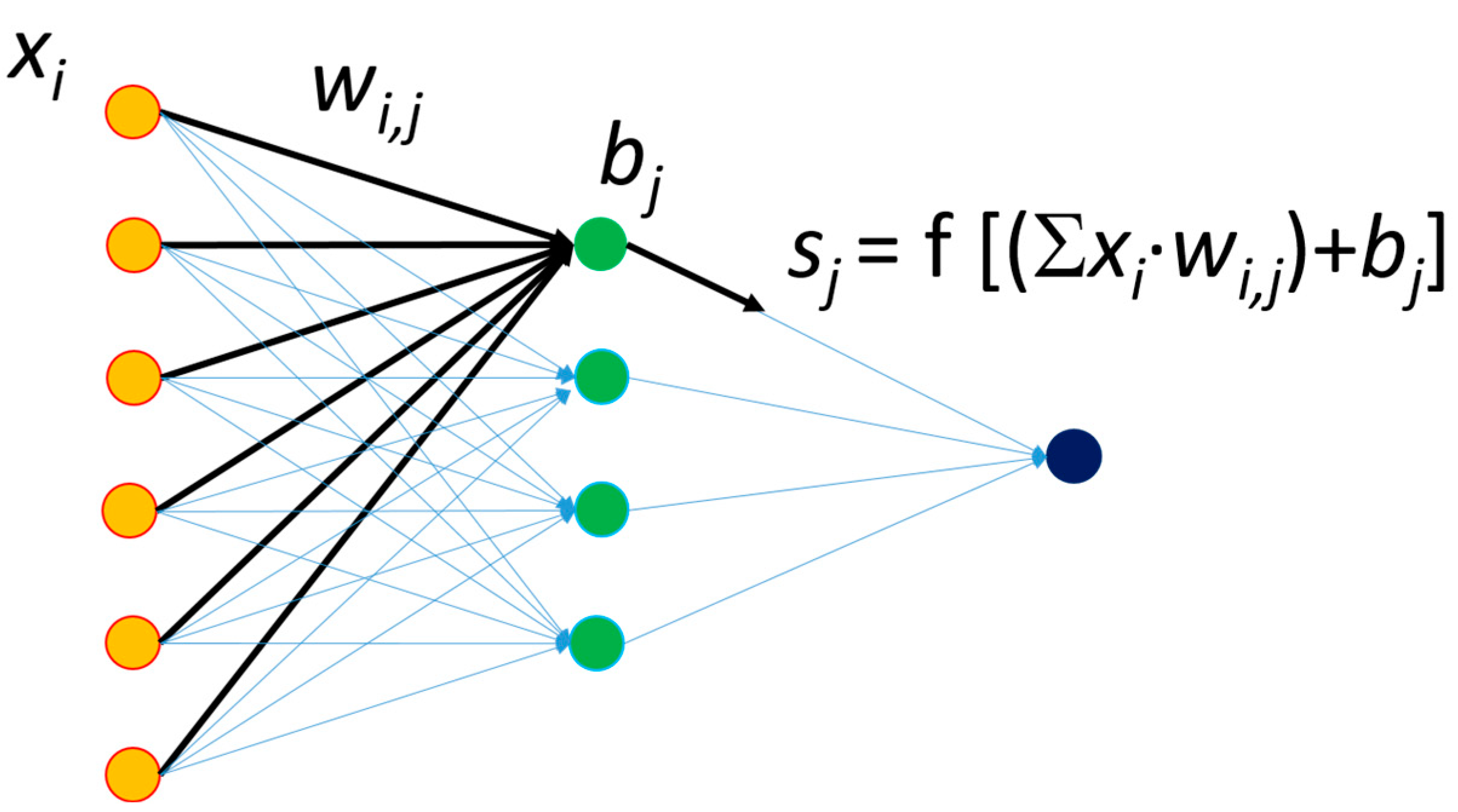
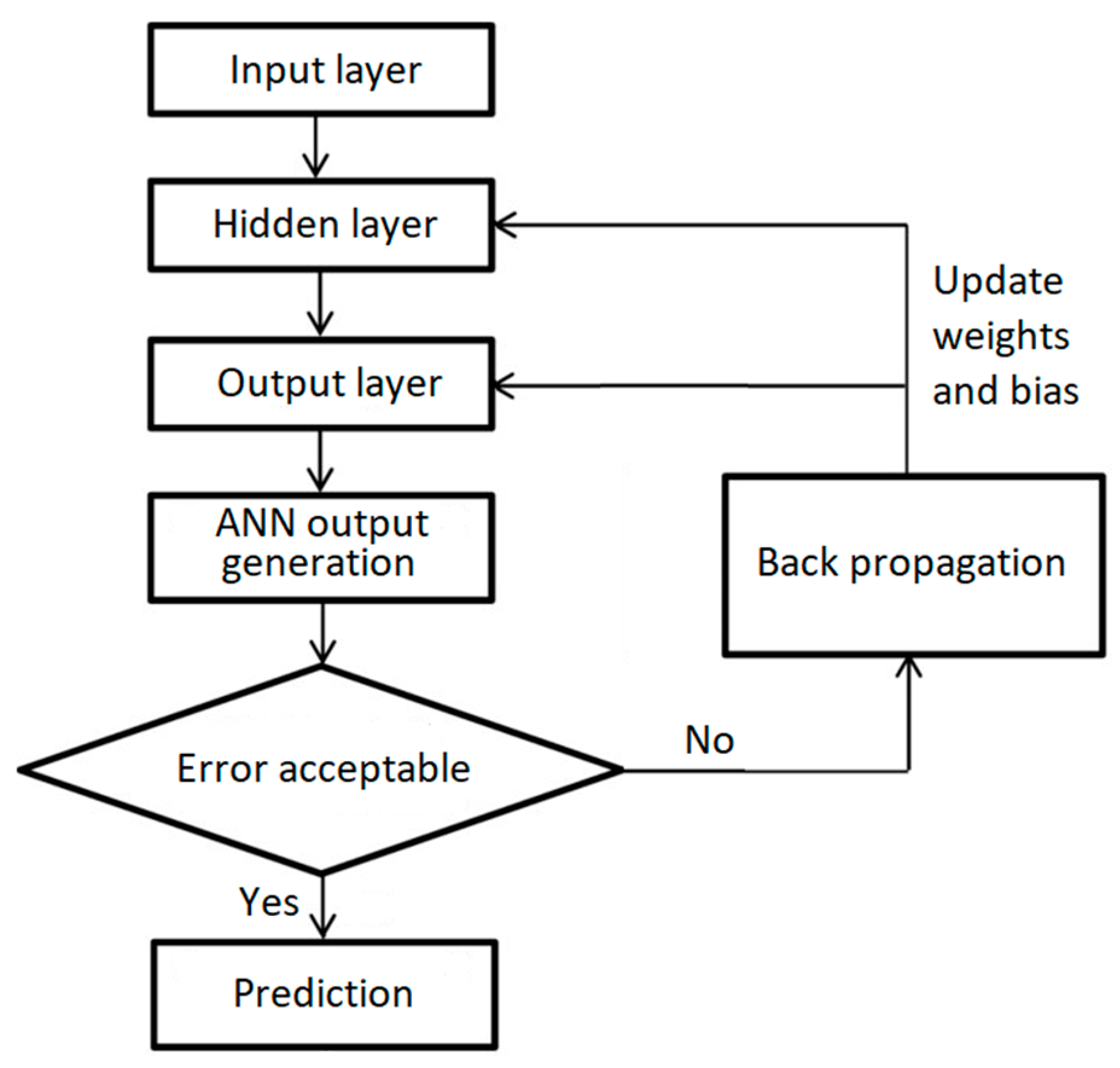
3.2. Artificial Neural Network

An artificial neural network (ANN) consists of neurons organized in layers (input, hidden, output) that detect complex relationships between variables. The input layer receives data, the hidden layer processes it, and the model is trained by adjusting weights iteratively. Errors are propagated backward to improve accuracy. LeCun et al. [30] thoroughly review the fundamental concepts, advancements, and applications of ANNs. Zhang et al. [31] provide an in-depth examination of how ANNs are applied to forecasting, detailing their effectiveness and methodologies in this domain.
A multilayer forward-fed network comprises a hidden layer of sigmoid neurons and an output layer of linear neurons. The neurons in the hidden layer connect to both input and output layers (Figure 5). The number of neurons in the input and output layers is proportional to the number of input and output parameters. The input variables, denoted by xi, are multiplied by the weighting coefficients, wi,j, and then combined linearly with an independent bias term, bj. The equation governing the behavior of each hidden neuron may be expressed as ∑xi · wi,j + bj. Subsequently, each neuron in the hidden layer generates an output by employing a sigmoid tangent function to the linear combination. The output layer employs a linear function.
The multilayer perceptron (MLP) network is a widely used model that approximates any function, even with a single hidden layer [30]. Its effectiveness stems from the backpropagation algorithm [32,33,34], which has various enhancements. This algorithm is essential for MLP’s application in classification and regression problems, particularly when training data with known target values are available.
In a forward-feeding neural network, the connections are unidirectional, moving from the input to the output layer, and the learning is supervised with data that have known responses. The data set is divided into three groups to evaluate overfitting: training data to adjust network parameters, validation data to detect overlearning during training, and test data used only at the end to assess performance. An “early stopping” technique prevents overfitting by dividing data into training and validation sets. During iterative optimization, the training and validation errors are compared. If the training error decreases while the validation error increases, the adjustment process is terminated to prevent overfitting.
The neural network used 42 data sets: 34 for training, 4 for validation, and 4 for testing, all chosen randomly. The network employed a five-neuron hidden layer. Performance is assessed through simulation, where data—either from training or new data for predictions—are input to examine the output.
The first step is cross-validation, comparing training output data with the neural network’s simulated output. This process is key to evaluating the network’s accuracy and detecting overfitting, where the model becomes too specialized to the training data and performs poorly on new data. Cross-validation can be applied to training, validation, testing, or all data to assess overfitting (Figure 6).
Figure 7 represents a network setting for the case studied, with cross-validation of training, validation, test, and total data. It must be noted that, on each occasion that the network is run, the data used for validation are chosen randomly, and the settings change each time. An analysis of the plots in Figure 7 shows that training the neural network on a random data set allows for a high correlation, which drops when the network is applied to new test data. This effect can also be seen when the network is applied to the entire data set used, where the R coefficient is high but lower in the training phase.

4. Results and Discussion

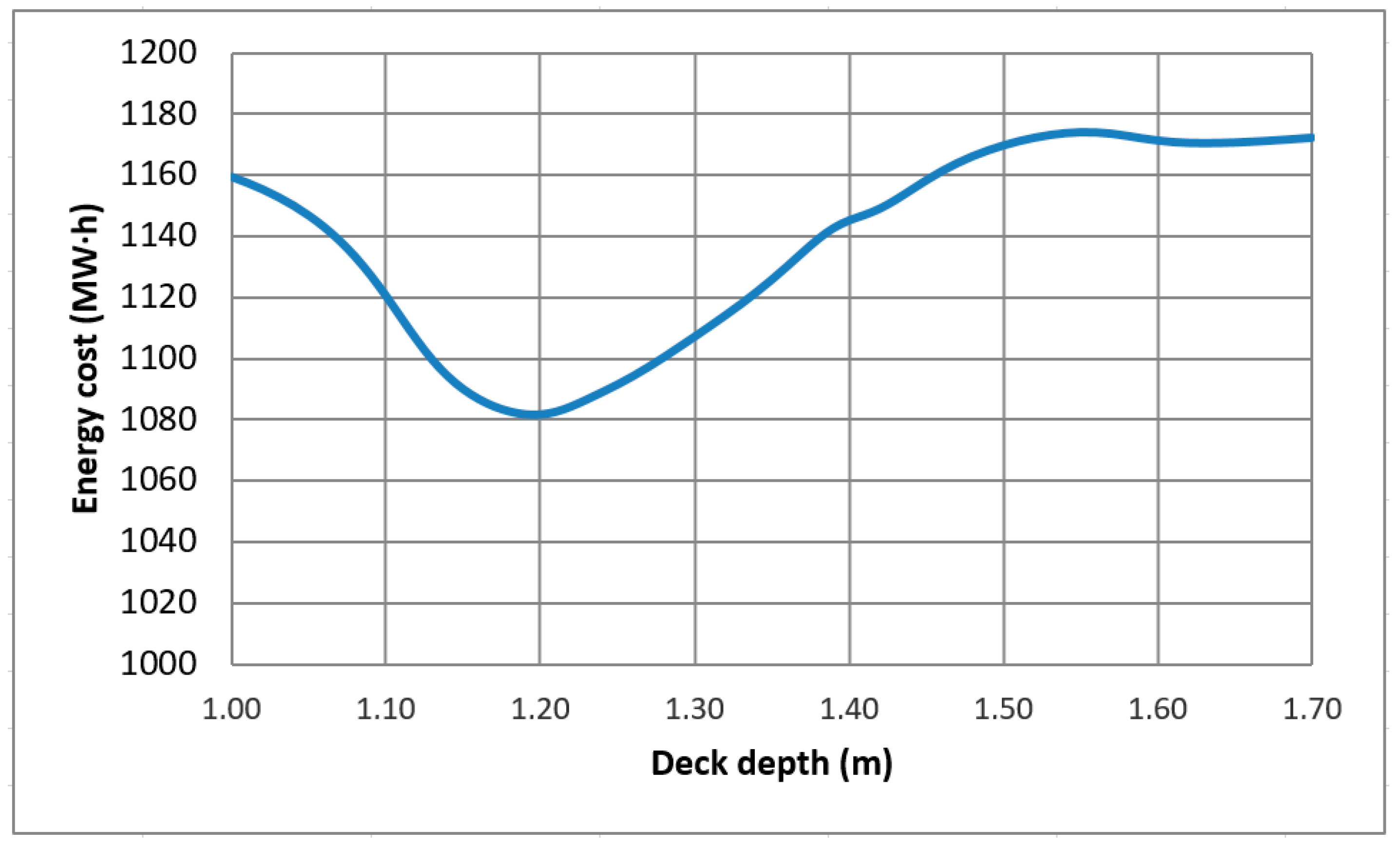
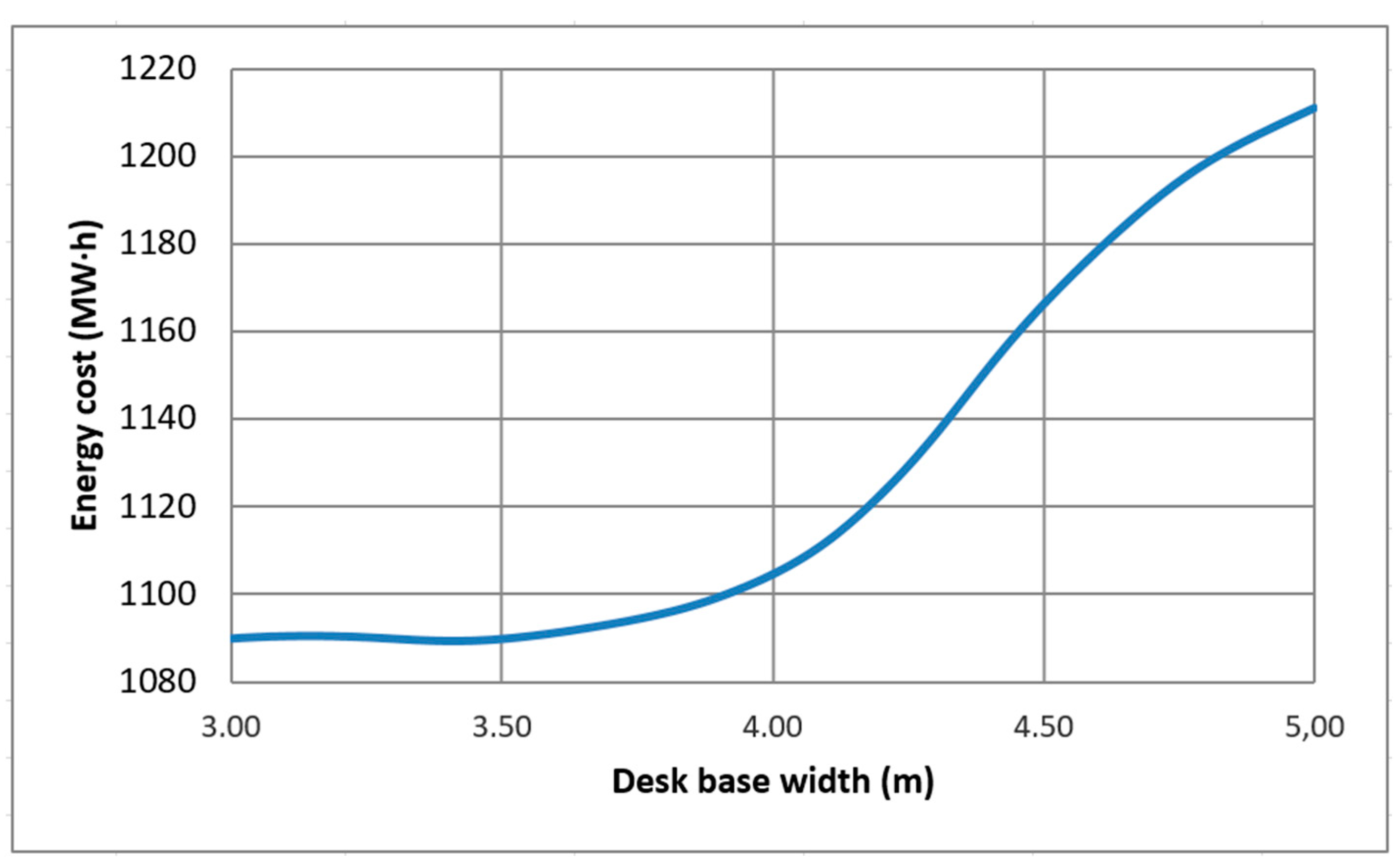
4.1. Visualization of Observed Data

Before applying the metamodels, the observed data can be plotted on a response surface to observe the abruptness of the response surface. Minitab v17 was used for this purpose. Figure 4 and Figure 8 plot the 42 observed data points (Table 2), with energy consumption represented as the response variable. Figure 8 depicts the contour plot corresponding to the observed data, revealing multiple local optima. Traditional linear regression models are inadequate, and even nonlinear models may overly smooth the response due to the surface’s abrupt nature. This complexity underscores the need for advanced predictive and optimization models to identify the optimal solution within this space.

4.2. Comparison of Predictive Models

Table 3 shows the observed values, the three Kriging models used, and the average of 16 neural network runs for the local optima obtained in the diversification (bridge #41) and intensification (bridge #42) phases of the response surface optimization. It is noted that Kriging predictive models are deterministic, while neural networks are not, because each time they are run, the data used for learning and validation are chosen randomly. Therefore, the neural network has been run 16 times to stabilize the standard deviation of the mean values (which is divided by 4).

4.3. Error Analysis

The predictive models show values above the observed data. The Kriging 3 model, which uses a regression polynomial of order 2, provides the lowest error. However, the average values predicted by 16 neural network runs give an error similar to the Kriging 2 model, which uses a regression polynomial of order 1.
However, the errors measured as mean square error (MSE) and root mean square error (RMSE) are lower for the neural network case (Table 4). The error values for the Kriging models’ case have been obtained for the prediction of values #31 to #42, while in the case of the neural network, they have been obtained using all 42 cases. Therefore, this supposed advantage of the neural networks is not homologous.
The subsequent step comprehensively examines the neural network’s capability to identify the optimal values. To accomplish this, we present the average values of the predictions made, as illustrated in Figure 7, Figure 8 and Figure 9 below.
Figure 10 illustrates the neural network’s accurate prediction of the deck depth’s minimum value, considering a 3.70 m base and 40 MPa concrete grade. Remarkably, a distinct minimum appears at a depth of 1.20 m, which notably aligns with the optimum obtained by Kriging.
When the depth of the deck remains at 1.20 m and the concrete grade is 40 MPa, the neural network indicates (Figure 11) that the minimum energy cost barely changes, with values ranging between 3.00 m and 3.50 m, and 3.35 m being the lowest.
Suppose a depth of the deck of 1.20 m and a base of 3.35 m are set. According to Figure 12, the neural network indicates that the value of the characteristic resistance offering the lowest energy cost is 41 MPa, which is close to the standardized value of 40 MPa used for constructing the structure.

4.4. Practical Recommendations

The Dirección General de Carreteras (DGC) [35] suggests a slenderness ratio between 1/22 and 1/30, while the SETRA [36] recommends a ratio of 1/28 for three-span slab decks with wide cantilevers. The outcomes of the neural network, which align with the conclusions of Yepes-Bellver et al. [22], provide practical recommendations for reducing emissions in a prestressed slab bridge comprising three spans with a main span of 34 m. These recommendations include a slenderness of about 1/28, a concrete content of between 0.55 m3/m2 and 0.60 m3/m2 for the deck, and a passive reinforcement content of between 100 kg/m3 and 130 kg/m3, with active reinforcement around 17 kg/m2 of the deck. The characteristic compressive strength of concrete should be at least 40 MPa, the internal lighting should not exceed 0.18 m3/m2 of the deck area, and the external lighting should be between 0.45 m3/m2 and 0.55 m3/m2 of the deck area.
Thus, the neural network can identify the local optimum, which is close to the value obtained after optimizing the response surface of the Kriging surrogate model. However, the Kriging models or neural networks must accurately determine the energy prediction. Therefore, while the surrogate models can provide a response surface, optimizing the response surface to find a local minimum is critical. However, these models allow for improved design results and help to narrow the optimal design ranges for critical variables. This proposed approach is a significant aid for structural engineers who refrain from routinely using heuristic optimization algorithms, resulting in missed opportunities to reduce economic and environmental costs.

5. Conclusions

This paper compares the performance of Kriging and a multilayer perceptron neural network for optimizing energy in prestressed lightweight slab bridges. Using 42 solutions from a real road overpass, the energy consumption required for its construction was evaluated using Kriging and neural network models. Verification revealed that the response surface assessing energy consumption is complex and steep, displaying numerous local optima, highlighting the problem’s complexity. Both Kriging models and neural networks tend to predict values above the observed ones. Specifically, the Kriging model, which uses polynomials of order 2, offers a relative error of 4% in the local optimum, which is lower than that of the neural network. However, the neural network demonstrates lower root mean square errors (RMSEs). Unlike deterministic Kriging models, neural networks require multiple runs to stabilize their responses and determine mean values. Furthermore, verification of this structural problem indicates that the neural network identifies the location of the local optimum, which closely resembles the value obtained from optimizing the Kriging response surface. However, neither the Kriging model nor the neural network achieves accurate predictions of the objective function; instead, they guide toward promising areas within the solution space. Therefore, while surrogate models establish a response surface, optimizing this surface to find a local minimum remains essential.

Author Contributions

This study represents a result of teamwork. Conceptualization, L.Y.-B., A.B.-I. and V.Y.; methodology, L.Y.-B., A.B.-I. and V.Y.; software, L.Y.-B. and J.A.; validation, L.Y.-B., A.B.-I. and J.A.; formal analysis, L.Y.-B., A.B.-I. and J.A.; investigation, L.Y.-B., A.B.-I., J.A. and V.Y.; resources, V.Y.; data curation, L.Y.-B. and A.B.-I.; writing—original draft preparation, L.Y.-B.; writing—review and editing, V.Y.; visualization, L.Y.-B. and A.B.-I.; supervision, J.A. and V.Y.; project administration, V.Y.; funding acquisition, V.Y. All authors have read and agreed to the published version of the manuscript.

Funding

Grant PID2023-150003OB-I00 funded by MCIN/AEI/10.13039/501100011033 and by “ERDF A way of making Europe”.

Informed Consent Statement

Not applicable.

Data Availability Statement

The original contributions presented in the study are included in the article, further inquiries can be directed to the corresponding author.

Acknowledgments

The authors wish to thank the editor of Sustainability and the anonymous reviewers for their valuable contributions in enhancing the earlier version of this manuscript.

Conflicts of Interest

The authors declare no conflicts of interest.

References

  1. IEA; UNEP. Global Status Report: Towards a Zero-Emission, Efficient and Resilient Buildings and Construction Sector; International Energy Agency and the United Nations Environment Programme: Paris, France, 2018. [Google Scholar]
  2. Wang, T.; Lee, I.S.; Kendall, A.; Harvey, J.; Lee, E.B.; Kim, C. Life cycle energy consumption and GHG emission from pavement rehabilitation with different rolling resistance. J. Clean Prod. 2012, 33, 86–96. [Google Scholar] [CrossRef]
  3. Wang, E.; Shen, Z. A hybrid Data Quality Indicator and statistical method for improving uncertainty analysis in LCA of complex system—Application to the whole-building embodied energy analysis. J. Clean Prod. 2013, 43, 166–173. [Google Scholar] [CrossRef]
  4. Halder, A.; Batra, S. Application of Predictive Analytics in Built Environment Research: A Comprehensive Bibliometric Study to Explore Knowledge Domains and Future Research Agenda. Arch. Computat. Methods Eng. 2023, 30, 4299–4324. [Google Scholar] [CrossRef]
  5. Opoku, D.G.J.; Agyekum, K.; Ayarkwa, J. Drivers of environmental sustainability of construction projects: A thematic analysis of verbatim comments from built environment consultants. Int. J. Constr. Manag. 2022, 22, 1033–1041. [Google Scholar] [CrossRef]
  6. Leonhardt, F. Prestressed Concrete: Design and Construction; Ernst & Sohn: Berlin, Germany, 1982. [Google Scholar]
  7. Warner, R.F.; Rangan, B.V.; Hall, A.S.; Faulkes, K.A. Concrete Structures; Longman: North Lakes, QLD, Australia, 1998. [Google Scholar]
  8. Yeo, D.; Gabbai, R.D. Sustainable design of reinforced concrete structures through embodied energy optimization. Energ. Buildings 2011, 43, 2028–2033. [Google Scholar] [CrossRef]
  9. Quaglia, C.P.; Yu, N.; Thrall, A.P.; Paolucci, S. Balancing energy efficiency and structural performance through multi-objective shape optimization: Case study of a rapidly deployable origami-inspired shelter. Energ. Buildings 2014, 82, 733–745. [Google Scholar] [CrossRef]
  10. Cabeza, L.F.; Boquera, L.; Chàfer, M.; Vérez, D. Embodied energy and embodied carbon of structural building materials: Worldwide progress and barriers through literature map analysis. Energy Build 2021, 231, 110612. [Google Scholar] [CrossRef]
  11. Miller, D.; Doh, J.H.; Mulvey, M. Concrete slab comparison and embodied energy optimisation for alternate design and construction techniques. Constr. Build Mater. 2015, 80, 329–338. [Google Scholar] [CrossRef]
  12. Foraboschi, P.; Mercanzin, M.; Trabucco, D. Sustainable structural design of tall buildings based on embodied energy. Energ. Buildings 2014, 68, 254–269. [Google Scholar] [CrossRef]
  13. Alcalá, J.; González-Vidosa, F.; Yepes, V.; Martí, J.V. Embodied energy optimization of prestressed concrete slab bridge decks. Technologies 2018, 6, 43. [Google Scholar] [CrossRef]
  14. Martí, J.V.; García-Segura, T.; Yepes, V. Structural design of prescast-prestressed concrete U-beam road bridges based on embodied energy. J. Clean. Prod. 2016, 120, 231–240. [Google Scholar] [CrossRef]
  15. Minunno, R.; O’Grady, T.; Morrison, G.M.; Gruner, R.L. Investigating the embodied energy and carbon of buildings: A systematic literature review and meta-analysis of life cycle assessments. Renew. Sustain. Energy Rev. 2021, 143, 110935. [Google Scholar] [CrossRef]
  16. Penadés-Plà, V.; García-Segura, T.; Yepes, V. Accelerated optimization method for low-embodied energy concrete box-girder bridge design. Eng. Struct 2019, 179, 556–565. [Google Scholar] [CrossRef]
  17. Cressie, N. The origins of Kriging. Math. Geol. 1990, 22, 239–252. [Google Scholar] [CrossRef]
  18. Martínez-Frutos, J.; Martí, P. Diseño óptimo robusto utilizando modelos Kriging: Aplicación al diseño óptimo robusto de estructuras articuladas. Rev. Int. Métodos Numér. Cálc. Diseño Ing. 2014, 30, 97–105. [Google Scholar] [CrossRef]
  19. YiFei, L.; MaoSen, C.; Hoa, T.N.; Khatir, S.; Minh, H.L.; SangTo, T.; Cuong-Le, T.; Wahab, M.A. Metamodel-assisted hybrid optimization strategy for model updating using vibration response data. Adv. Eng. Softw. 2023, 185, 103515. [Google Scholar] [CrossRef]
  20. Sánchez-Zabala, V.F.; Gómez-Acebo, T. Building energy performance metamodels for district energy management optimisation platforms. Energy Convers. Manag. X 2024, 21, 100512. [Google Scholar] [CrossRef]
  21. Yepes-Bellver, L.; Brun-Izquierdo, A.; Alcalá, J.; Yepes, V. CO2-optimization of post-tensioned concrete slab-bridge decks using surrogate modeling. Materials 2022, 15, 4776. [Google Scholar] [CrossRef]
  22. Yepes-Bellver, L.; Brun-Izquierdo, A.; Alcalá, J.; Yepes, V. Embodied energy optimization of prestressed concrete road flyovers by a two-phase Kriging surrogate model. Materials 2023, 16, 6767. [Google Scholar] [CrossRef]
  23. Zhang, Y.; Wu, G. Seismic vulnerability analysis of RC bridges based on Kriging model. J. Earthq. Eng. 2019, 23, 242–260. [Google Scholar] [CrossRef]
  24. Wu, J.; Cheng, F.; Zou, C.; Zhang, R.; Li, C.; Huang, S.; Zhou, Y. Swarm intelligent optimization conjunction with Kriging model for bridge structure finite element model updating. Buildings 2022, 12, 504. [Google Scholar] [CrossRef]
  25. Cheng, A.; Low, Y.M. A new metamodel for predicting the nonlinear time-domain response of offshore structures subjected to stochastic wave current and wind loads. Comput. Struct. 2024, 297, 107340. [Google Scholar] [CrossRef]
  26. Martí-Vargas, J.R.; Ferri, F.J.; Yepes, V. Prediction of the transfer length of prestressing strands with neural networks. Comput. Concr. 2013, 12, 187–209. [Google Scholar] [CrossRef]
  27. Hong, W.K.; Nguyen, M.C.; Pham, T.D. Pre-tensioned concrete beams optimized with a unified function of objective (UFO) using ANN-based Hong-Lagrange method. J. Asian Archit. Build Eng. 2023, 23, 1573–1595. [Google Scholar] [CrossRef]
  28. Lophaven, N.S.; Nielsen, H.B.; Sondergaard, J. MATLAB Kriging Toolbox DACE (Design and Analysis of Computer Experiments) Version 2.0. 2002. Available online: http://www2.imm.dtu.dk/pubdb/p.php?1460 (accessed on 11 July 2024).
  29. McKay, M.D.; Beckman, R.J.; Conover, W.J. A Comparison of Three Methods for Selecting Values of Input Variables in the Analysis of Output from a Computer Code. Technometrics 1979, 21, 239–245. [Google Scholar] [CrossRef]
  30. LeCun, Y.; Bengio, Y.; Hinton, G. Deep Learning. Nature 2015, 521, 436–444. [Google Scholar] [CrossRef]
  31. Zhang, G.; Patuwo, B.E.; Hu, M.Y. Forecasting with artificial neural networks: The state of the art. Int. J. Forecast 1998, 14, 35–62. [Google Scholar] [CrossRef]
  32. Hornik, K.; Stinchcombe, M.; White, H. Multilayer feedforward networks are universal approximator. Neural Netw. 1989, 2, 359–366. [Google Scholar] [CrossRef]
  33. Rumelhart, D.E.; McClelland, J.L.; PDP Research Group. Parallel Distributed Processing: Explorations in the Microstructure of Cognition; MIT Press: Cambridge, UK, 1986; Volume 1. [Google Scholar] [CrossRef]
  34. Rumelhart, D.E.; Hinton, G.E.; Williams, R.J. Learning Representations by Back-Propagating Errors. Nature 1986, 323, 533–536. [Google Scholar] [CrossRef]
  35. Dirección General de Carreteras. Obras de paso de Nueva Construcción: Conceptos Generales; Ministerio de Fomento, Centro de Publicaciones: Madrid, Spain, 2000. (In Spanish)
  36. SETRA. Ponts-Dalles. Guide de Conception; Ministère de l’Equipement, du Logement des Transports et de la Mer: Bagneux, France, 1989. (In French)
Figure 1. Longitudinal profile of the PC slab road bridge [21,22].
Sustainability 16 08450 g001
Figure 2. Cross-sectional view of the lightweight PC slab bridge deck [21,22].
Sustainability 16 08450 g002
Figure 3. Aerial image of the overpass at kilometer 441 of the A-7 highway in Cocentaina (Alicante). Image: Google Maps.
Sustainability 16 08450 g003
Figure 4. Example of response surface.
Sustainability 16 08450 g004
Figure 5. Example of a neural network with a hidden layer.
Sustainability 16 08450 g005
Figure 6. ANN model flowchart.
Sustainability 16 08450 g006
Figure 7. Cross-validation of training data, validation, test, and total data.
Sustainability 16 08450 g007
Figure 8. Response surface of the 42 observed slab bridge deck data (Table 2).
Sustainability 16 08450 g008
Figure 9. Contour plot of the 42 observed slab data (Table 2).
Sustainability 16 08450 g009
Figure 10. ANN energy cost prediction as a function of deck depth, considering a 3.70 m base width and 40 MPa concrete grade.
Sustainability 16 08450 g010
Figure 11. ANN energy cost prediction as a function of deck depth width, considering a 1.20 m depth and 40 MPa concrete grade.
Sustainability 16 08450 g011
Figure 12. ANN energy cost prediction as a function of the concrete grade, considering a 1.20 m depth and 3.35 m base width.
Sustainability 16 08450 g012
Table 1. Energy cost of the deck [16].
MaterialkWh/kgkWh/m3kWh/m2
Y-1860-S7 steel5.64
B-500-St steel3.03
Lighting 604.42
Slab formwork 2.24
C-30 concrete 227.01
C-35 concrete 263.96
C-40 concrete 298.57
C-45 concrete 330.25
C-50 concrete 358.97
Lighting 604.42
Slab formwork 2.24
Table 2. Values of design variables obtained within the specified ranges [22].
DeckDeck Depth (m)Base
Width (m)
Concrete
Grade (MPa)
Energy Cost
(MW·h)
11.653.65351149.88
21.703.80451182.89
31.203.85401065.87
41.553.60451140.79
51.204.85501170.72
61.154.50501199.59
71.353.95301103.18
81.304.45301180.31
91.354.25451132.71
101.504.55301138.00
111.604.20401267.85
121.254.70401191.65
131.504.05451183.17
141.454.35351119.17
151.653.45451145.07
161.554.10351162.92
171.253.50451073.75
181.403.30401152.33
191.453.90451145.21
201.353.60351094.86
211.503.35451134.93
221.504.50451189.53
231.553.20301103.41
241.253.00501101.04
251.403.45451201.73
261.503.55351105.44
271.703.85451165.47
281.203.60401083.41
291.304.90401215.82
301.454.75351163.59
311.203.40401059.87
321.153.90351129.22
331.053.50351237.89
341.103.80451178.72
351.153.35451074.77
361.253.60451078.71
371.103.45401124.21
381.203.35451065.44
391.253.40451084.92
401.153.60451104.77
411.153.35401051.00
421.153.70401038.28
Table 3. Observed value and prediction for local optima in diversification (#41) and intensification phase (#42), as well as their absolute and relative errors.
#41#42Absolute Error #41Relative Error #41Absolute Error #42Relative Error #42
Observed1051.001038.280.000.00%0.000.00%
Kriging 11130.681091.9579.687.58%53.675.17%
Kriging 21073.981085.8422.982.19%47.564.58%
Kriging 31060.581079.819.580.91%41.534.00%
ANN average1073.061091.8522.062.10%53.575.16%
Table 4. MSE and RMSE errors of the predictive models used.
Predictive ModelsMSERMSE
Kriging 12212.9847.04
Kriging 23923.4962.64
Kriging 34976.8070.55
ANN average1037.2230.95
Disclaimer/Publisher’s Note: The statements, opinions and data contained in all publications are solely those of the individual author(s) and contributor(s) and not of MDPI and/or the editor(s). MDPI and/or the editor(s) disclaim responsibility for any injury to people or property resulting from any ideas, methods, instructions or products referred to in the content.

