
Dynamic Optimization and Placement of Renewable Generators and Compensators to Mitigate Electric Vehicle Charging Station Impacts Using the Spotted Hyena Optimization Algorithm

 ,
,  ,
,  ,
,  and
and
Abstract
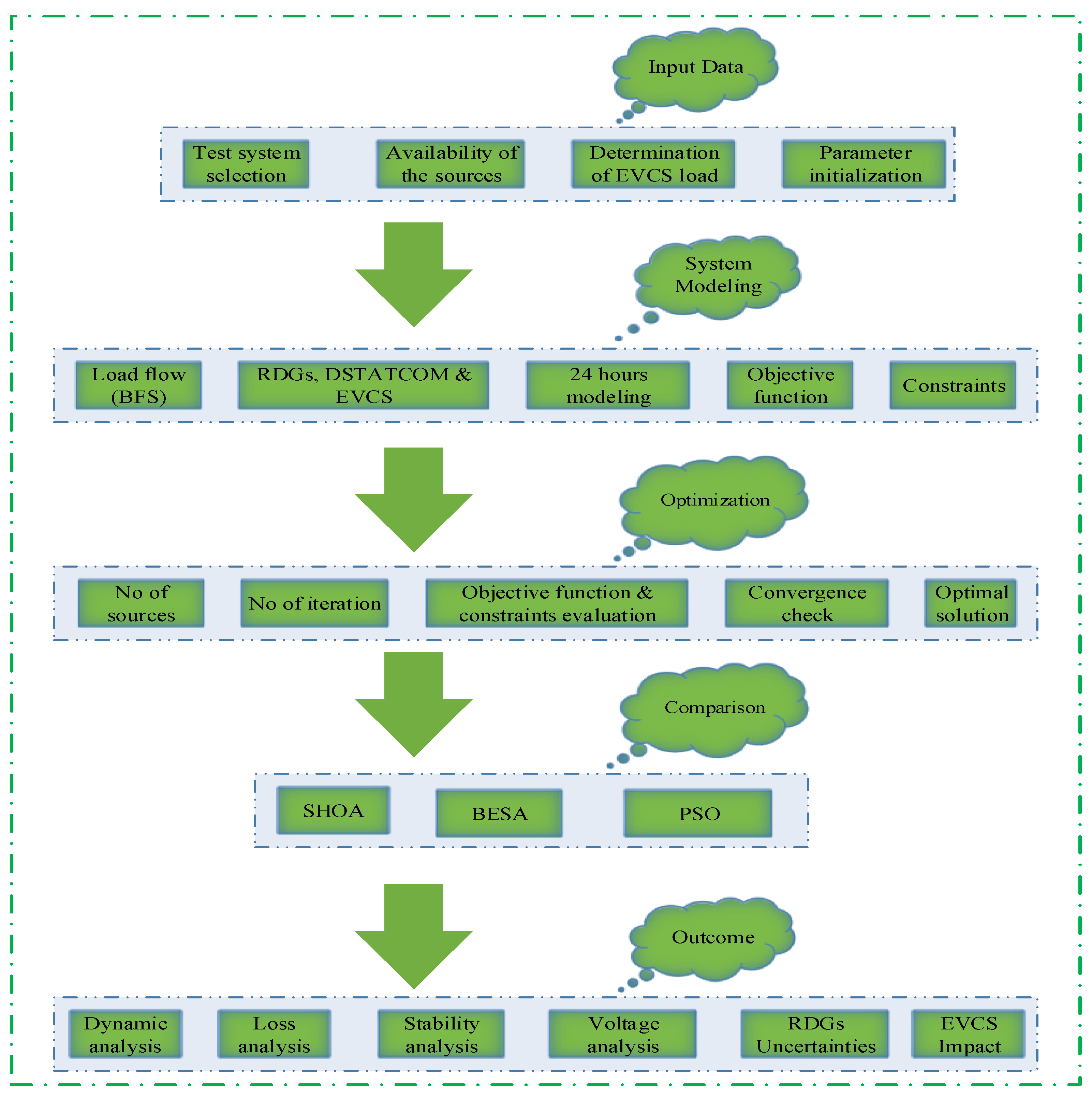
:1. Introduction
1.1. Motivation and Concept
1.2. Literature Review
1.3. Research Gaps
1.4. Research Contribution
- Utilizing a novel nature-inspired SHOA for the dynamic allocation of solar and wind-based RDG and DSTATCOMs, effectively minimizing the impact of EVCSs on the RDS.
- Identifying near-global optimum locations and sizes for RDG, DSTATCOMs, and EVCSs operating in both G2V and V2G modes to minimize power loss while adhering to system constraints.
- Evaluating the SHOA’s effectiveness in constant load scenarios using various optimization algorithms for EVCSs, RDG, and DSTATCOMs allocation.
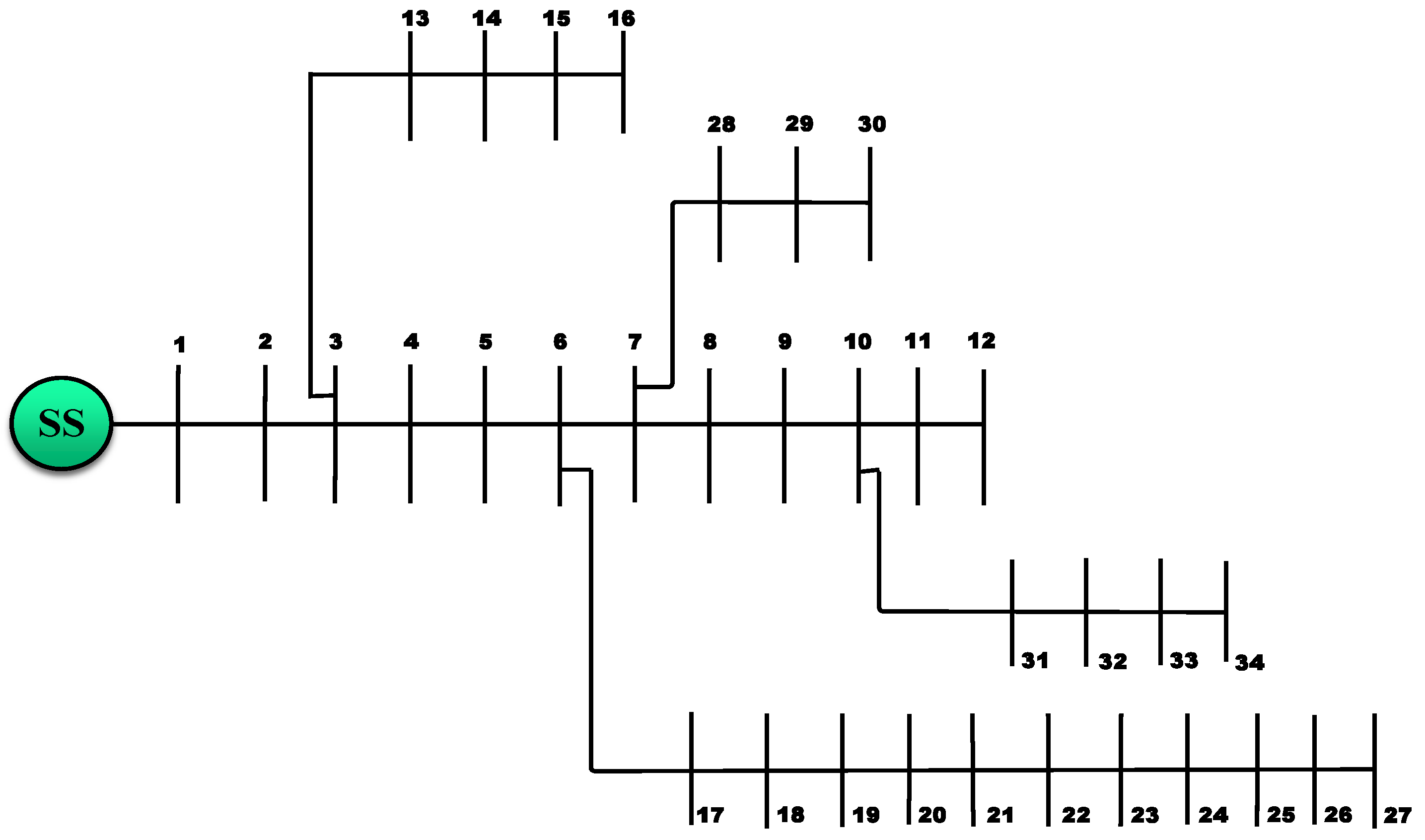
- Applying the SHOA to the IEEE 34-bus system to provide practical insights into system performance and resource distribution.
1.5. Structure of the Paper
2. Formulation of Problem
2.1. Power Flow Analysis
- (a)
- Total Real Power Loss over 24 h
- (b)
- Total Reactive Power Loss over 24 h
2.2. Voltage Stability Index
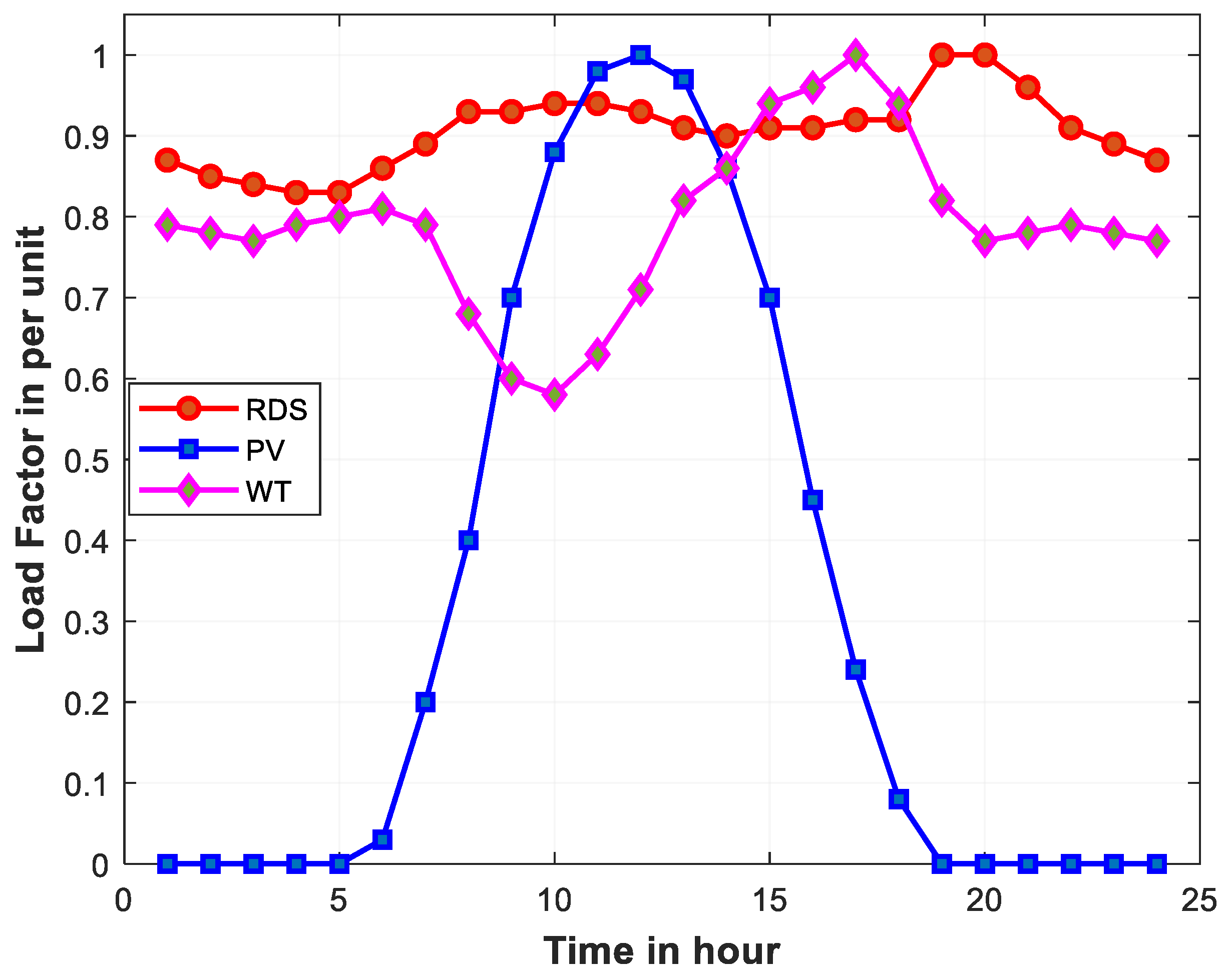
2.3. Modeling the Energy Sources for the RDS
2.3.1. PV Modeling for a 24-h Period
2.3.2. WT Modeling for a 24-h Period
2.3.3. Modeling of RDG for a 24-h Period
2.3.4. Modeling of DSTATCOMs for a 24-h Period
2.3.5. Modeling of EVCSs for a 24-h Period
- (i)
- Load Calculation Including EVCSs
- (ii)
- Charging and Discharging Characteristics
- (a)
- Charging Power Calculation (G2V Mode): The power required for charging EV batteries at hour n in G2V mode is calculated as follows:In the equation presented above, is the total charging power at hour n. represents the battery capacity of each EV in kilowatt-hours (kWh). is the change in State of Charge (SOC) for EV ‘i’ at hour n, measured in ampere-hours (Ah). is the charging coefficient for EV ‘i’, reflecting variations in charging power based on SOC and charger type.
- (b)
- Discharging Power Calculation (V2G Mode): The power required for discharging EV batteries at hour n in V2G mode is calculated as follows:In the equation presented above, is the total discharging power at hour n. is the discharging coefficient for EV ‘i’, reflecting the power delivered during discharging.
- (c)
- Idle Power Calculation: When EVCSs are idle, there is no power draw or supply from the EVCS. The power during idle periods is the following:This equation indicates that no additional load or supply is associated with idle EVCSs.
- (iii)
- Considerations for Accurate ModelingTo ensure the accuracy and relevance of the simulation study, it is crucial to consider various factors that influence the performance of EVCSs, RDG, and DSTATCOMs within an RDS. This section addresses key aspects such as charging characteristics, battery capacity standards, operational modes, and optimization techniques, while incorporating practical capacity limits for equipment used in the IEEE 34-bus RDS [34,35,36,37].
- (a)
- Charging characteristics: Accurate modeling of EVCSs requires accounting for non-linear charging profiles. As vehicles near higher SOC levels, the charging power typically decreases, following a non-linear curve. SOC is measured in ampere-hours (Ah). Detailed charging curves should therefore replace simplified linear models. For this study, the practical capacity ranges for chargers are considered, with Level 2 chargers providing between 3.7 kW and 22 kW, and DC fast chargers delivering up to 350 kW.
- (b)
- Battery capacity and charging standards: Battery capacity assumptions must align with current market standards. Modern EV batteries generally exceed 40 kWh, with capacities ranging between 40 kWh and 100 kWh depending on the vehicle model. Charging power is influenced by both battery capacity and the type of charger used. Standard home chargers (Level 1 or Level 2) offer up to 22 kW, while rapid DC chargers can provide up to 350 kW. These factors are crucial for accurate modeling to reflect real-world conditions.
- (c)
- G2V and V2G modes: The model incorporates both G2V and V2G modes. G2V mode involves charging the vehicle from the grid, whereas V2G mode allows the vehicle to discharge power back to the grid. Effective modeling of V2G requires accounting for bidirectional power flows, which can impact grid stability and vehicle battery health. Configurations for EVCSs should be evaluated to manage these modes efficiently.
- (d)
- Optimization: The SHOA was employed to determine the optimal allocation of EVCSs within the RDS. This algorithm identifies the most effective locations to minimize total load impacts and enhance system performance. The optimization process integrates factors such as charging and discharging characteristics, battery capacities, and charger types to ensure optimal placement and operation throughout the 24-h period.
2.4. Objective Function
2.5. System Constraints
- Power Balance Constraint
- (i)
- In G2V Mode
- (ii)
- In V2G Mode
- b.
- Voltage Magnitude Constraint
- c.
- Real Power Compensation
- d.
- Reactive Power Compensation
- e.
- SOC Limits for EVCS
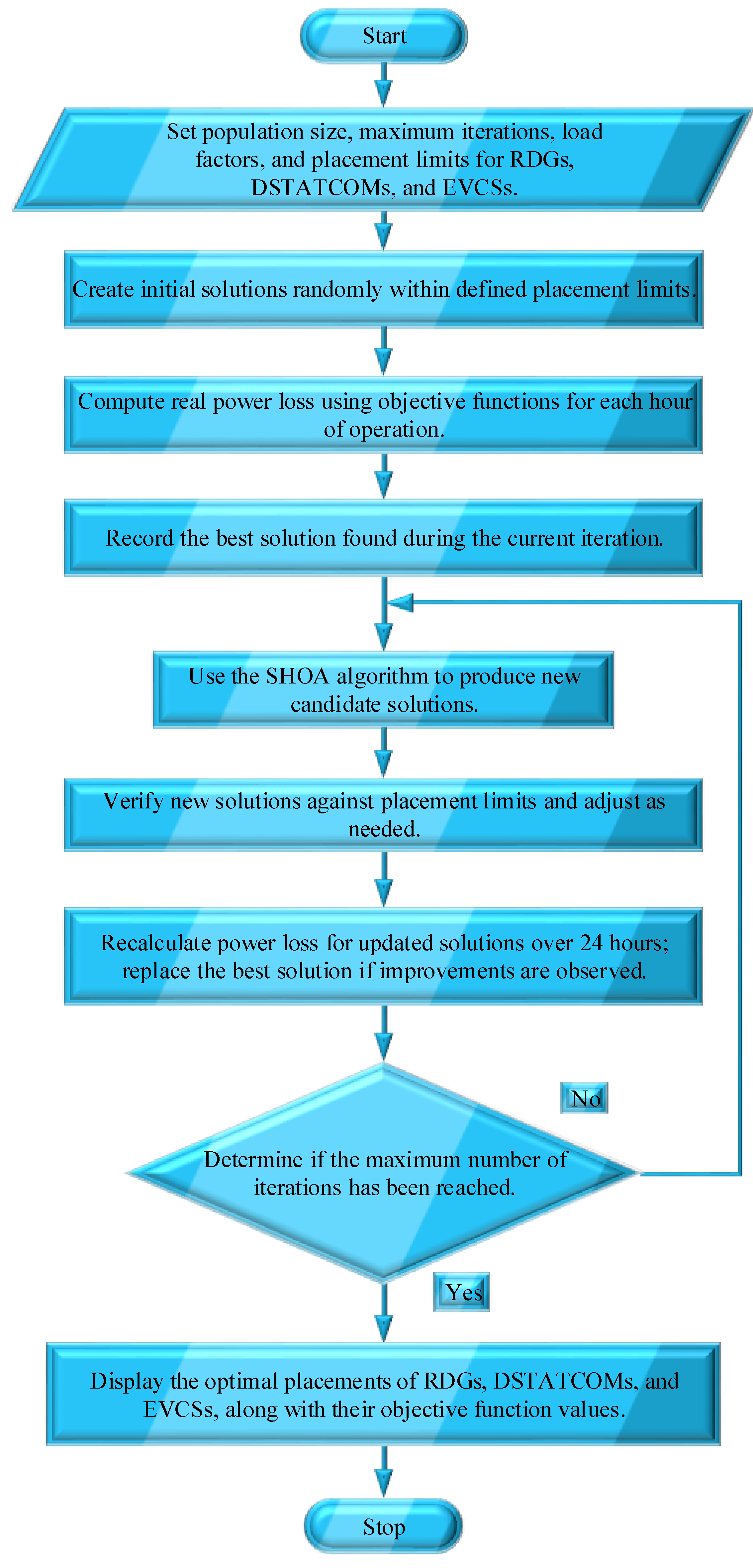
3. Spotted Hyena Optimization Algorithm
3.1. Introduction of SHOA
3.2. Algorithm Parameters
- (i)
- Parameters: The SHOA used a population size of 50 with 100 iterations. The crossover probability was 0.8, mutation probability 0.2, and selection pressure 2.
- (ii)
- Constraint Handling: A penalty function, summing the squared deviations of voltage and current from their limits, was applied to enforce constraints.
- (iii)
- Convergence Criteria: Convergence was achieved when the average fitness value remained unchanged for 10 iterations, with a criterion of 10−6.
- (iv)
- Initial Conditions: The initial population was randomly generated with values set to 0.5 p.u.
- (v)
- Experimental Data: dynamic load model load factors data were sourced from [10].
3.3. SHOA Steps
- (i)
- Encircling prey: The approach incorporates the consideration of various search factors and continuously updates the near global optimum position in response to the target. The mathematical model used to represent this behavior is expressed through a specific equation, which can differ based on the specific optimization problem at hand.
- (ii)
- Hunting: The SHOA hunting strategy can be described as follows:
- (iii)
- Attacking prey (exploitation): The mathematical expression for the process of prey attack is as follows:
- (iv)
- Search for prey (exploration): To find the right solution, the value of Z in Equation (35) must be either more than or less than one. The vector Y is another SHOA component that helps with exploration. Vector Y consists of randomly generated values that assign random weights to the prey. The elements in the Y vector that are greater than 1 are given higher priority than those less than 1. This prioritization highlights the unpredictable nature of the SHOA and the influence of distance in the optimization process.
- (v)
- Adaptive stopping criterion: The adaptive stopping criterion can be integrated into the main loop of the SHOA, typically after the iteration progress is monitored and updated. This check can be performed at the end of each iteration to determine whether to halt further iterations. By incorporating an adaptive stopping criterion into the SHOA, you can improve its efficiency and prevent unnecessary computation when convergence is reached or when further iterations no longer yield significant improvements in the objective function.
4. Results and Discussion
4.1. Simulation Study
- (i)
- Before Compensation
- (ii)
- After Compensation
- (i)
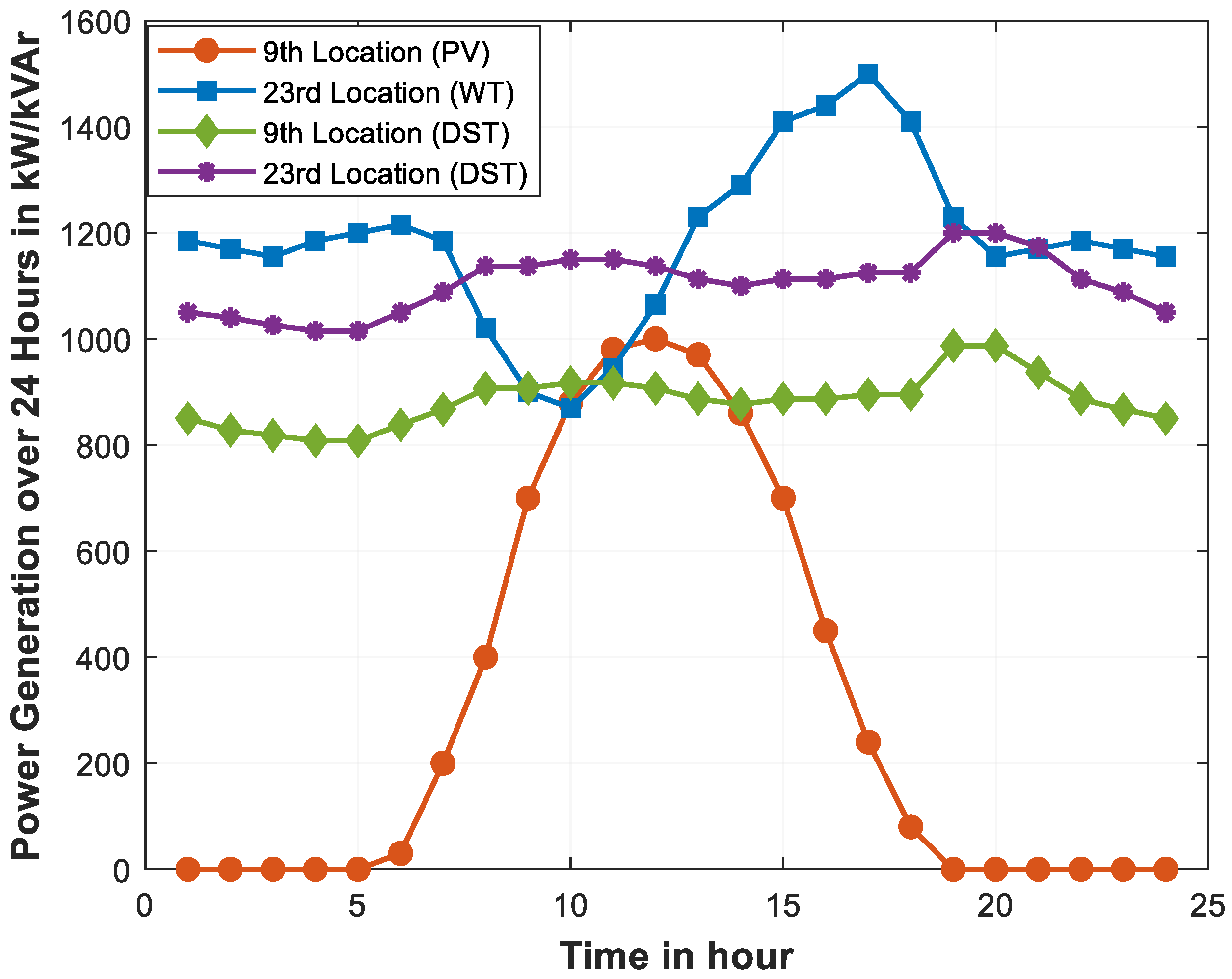
- WT-based RDG: maximum capacity: 1500 kW, minimum capacity: 50 kW
- (ii)
- PV-based RDG: maximum capacity: 1000 kW, minimum capacity: 30 kW
- (iii)
- DSTATCOM: maximum capacity: 1200 kVAr, minimum capacity: 50 kVAr
- (iv)
- EVCS: maximum charging power: 350 kW (DC fast charger), minimum charging power: 7.4 kW (Level 2 charger)
4.2. Simulation Findings and Discussion
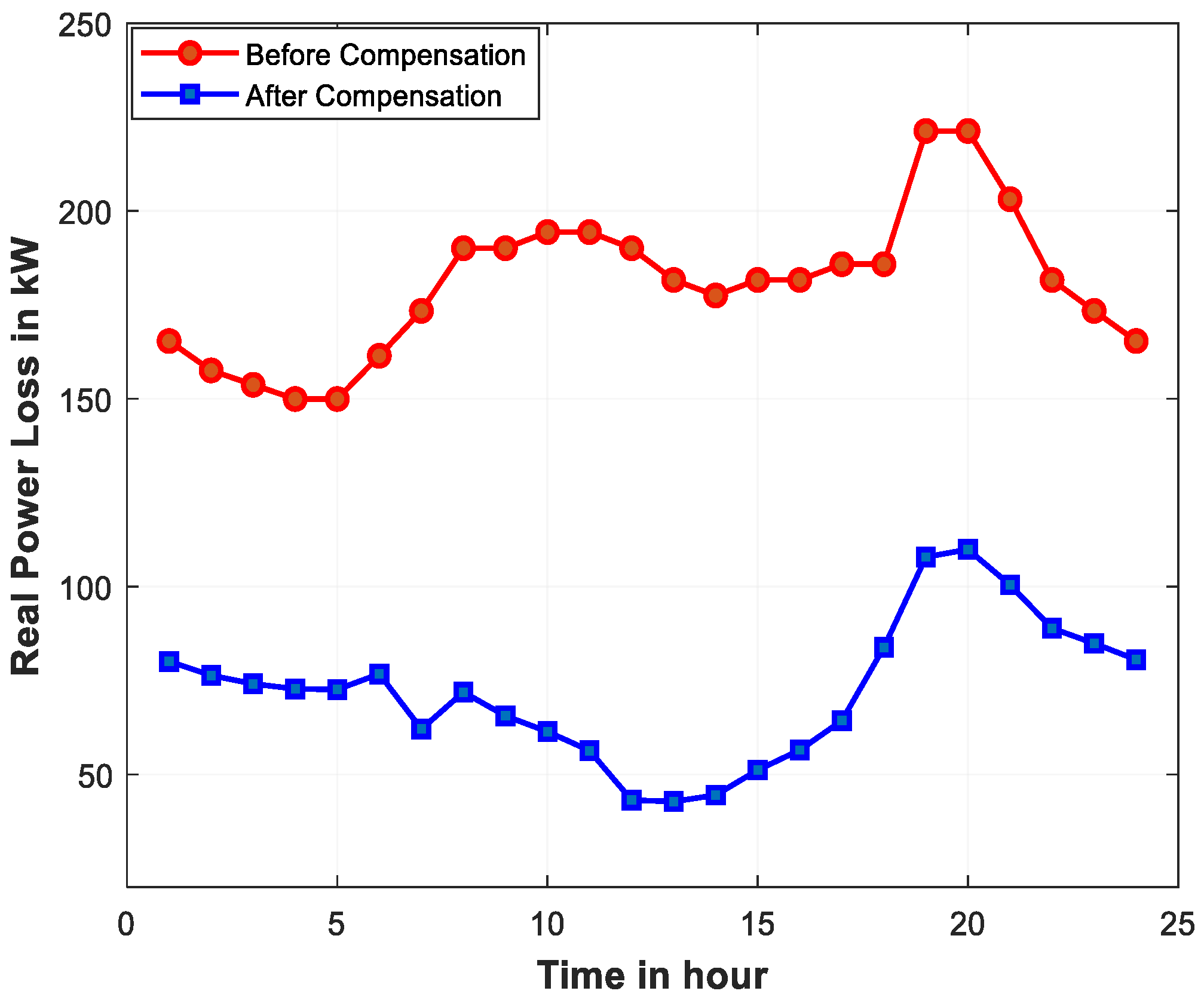
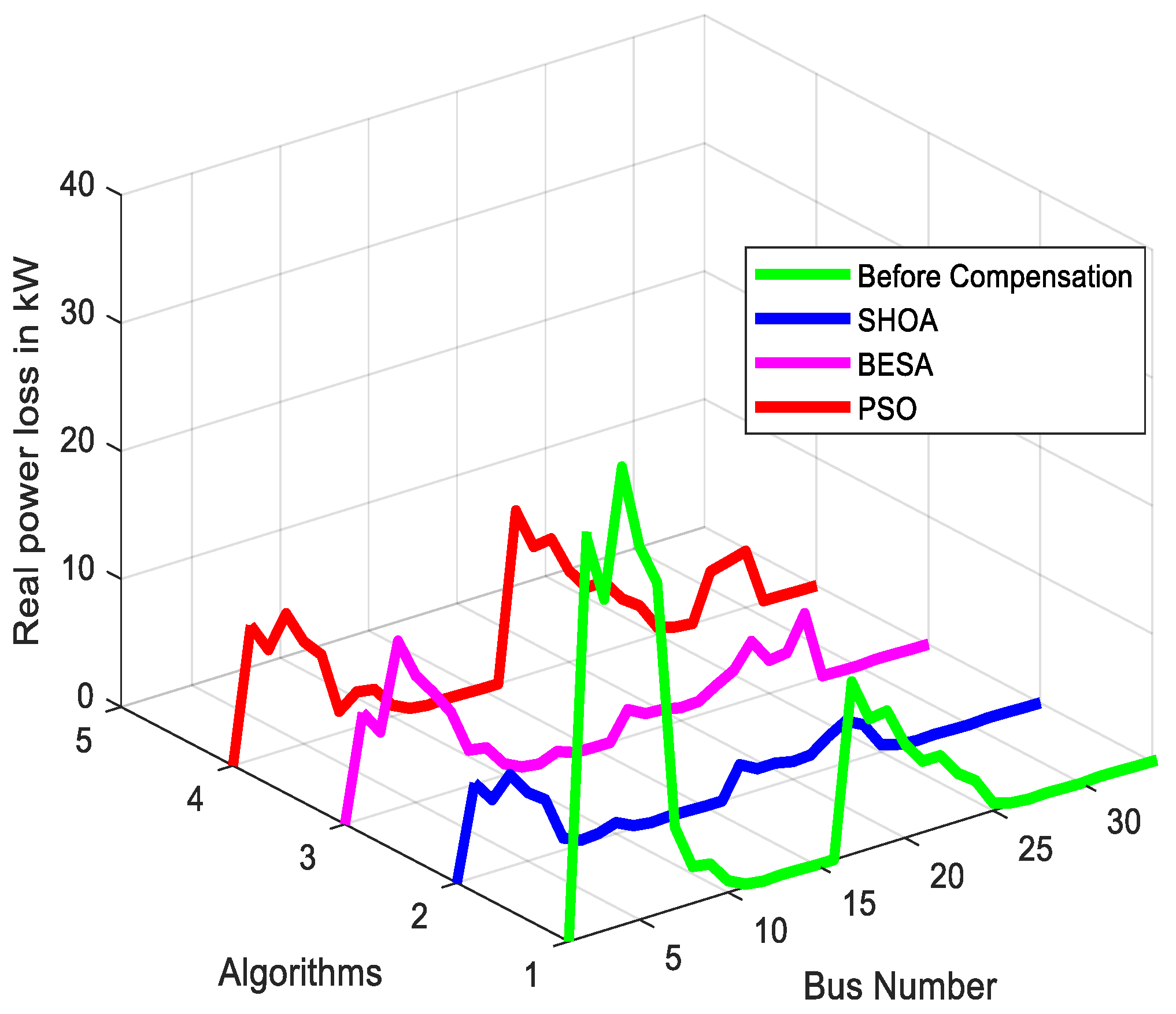
- (i)
- Real Power Loss Reduction
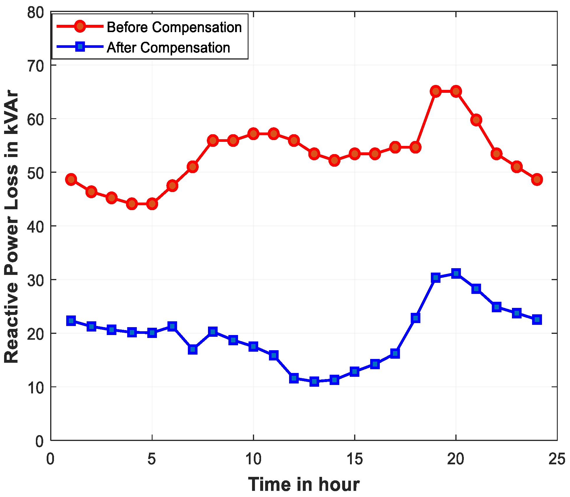
- (ii)
- Reactive Power Loss Reduction
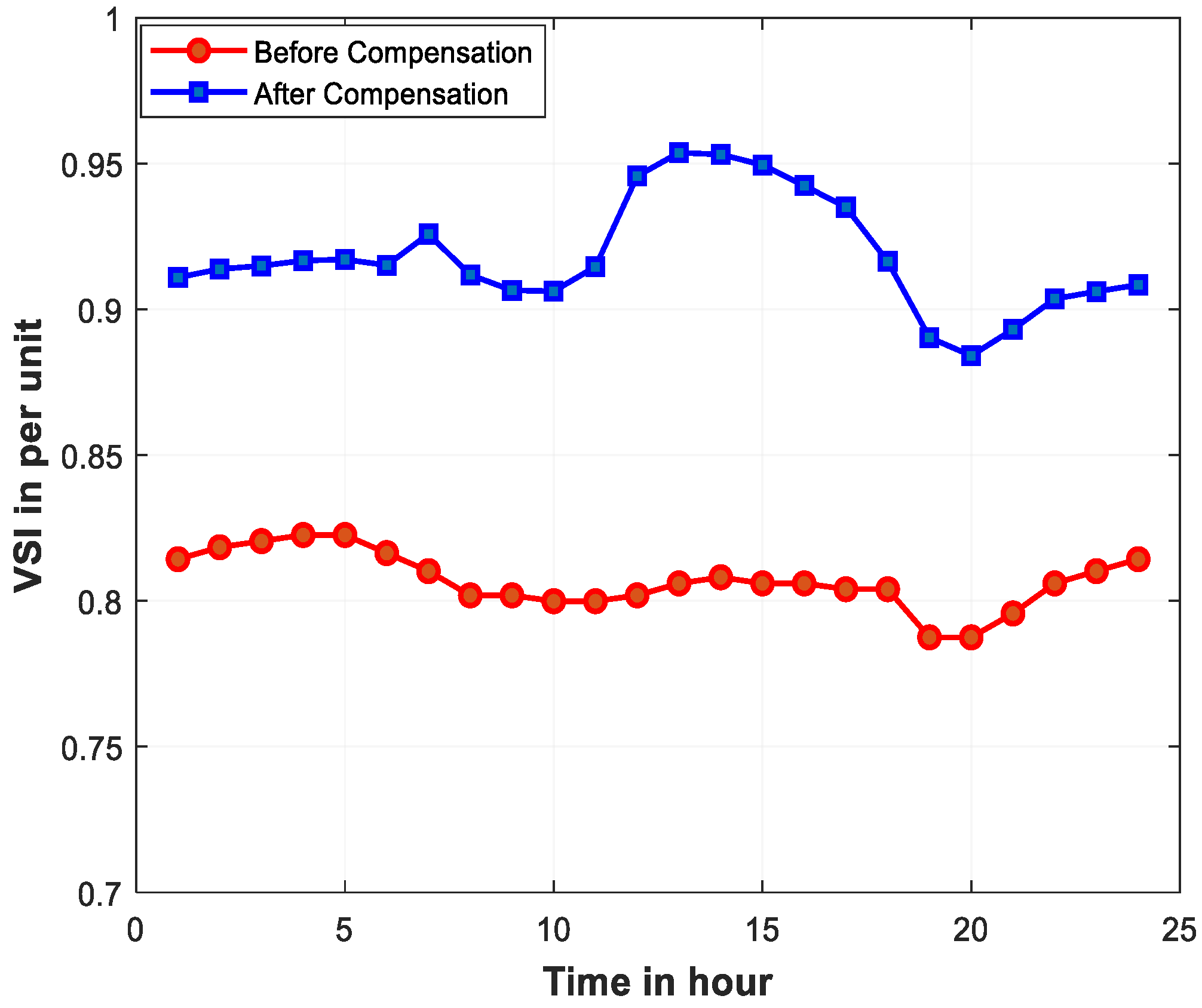
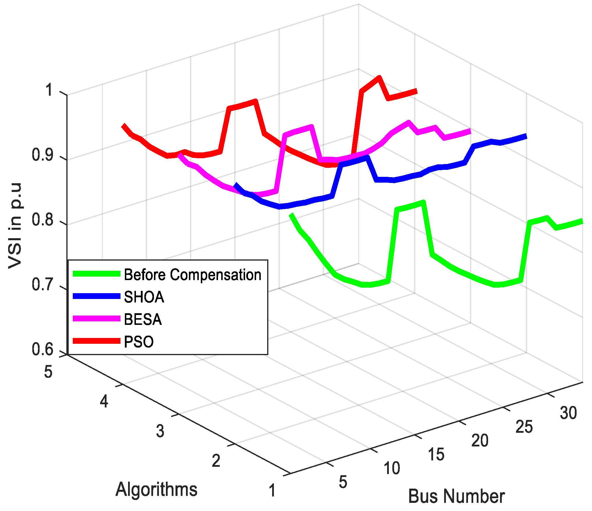
- (iii)
- VSI Improvement
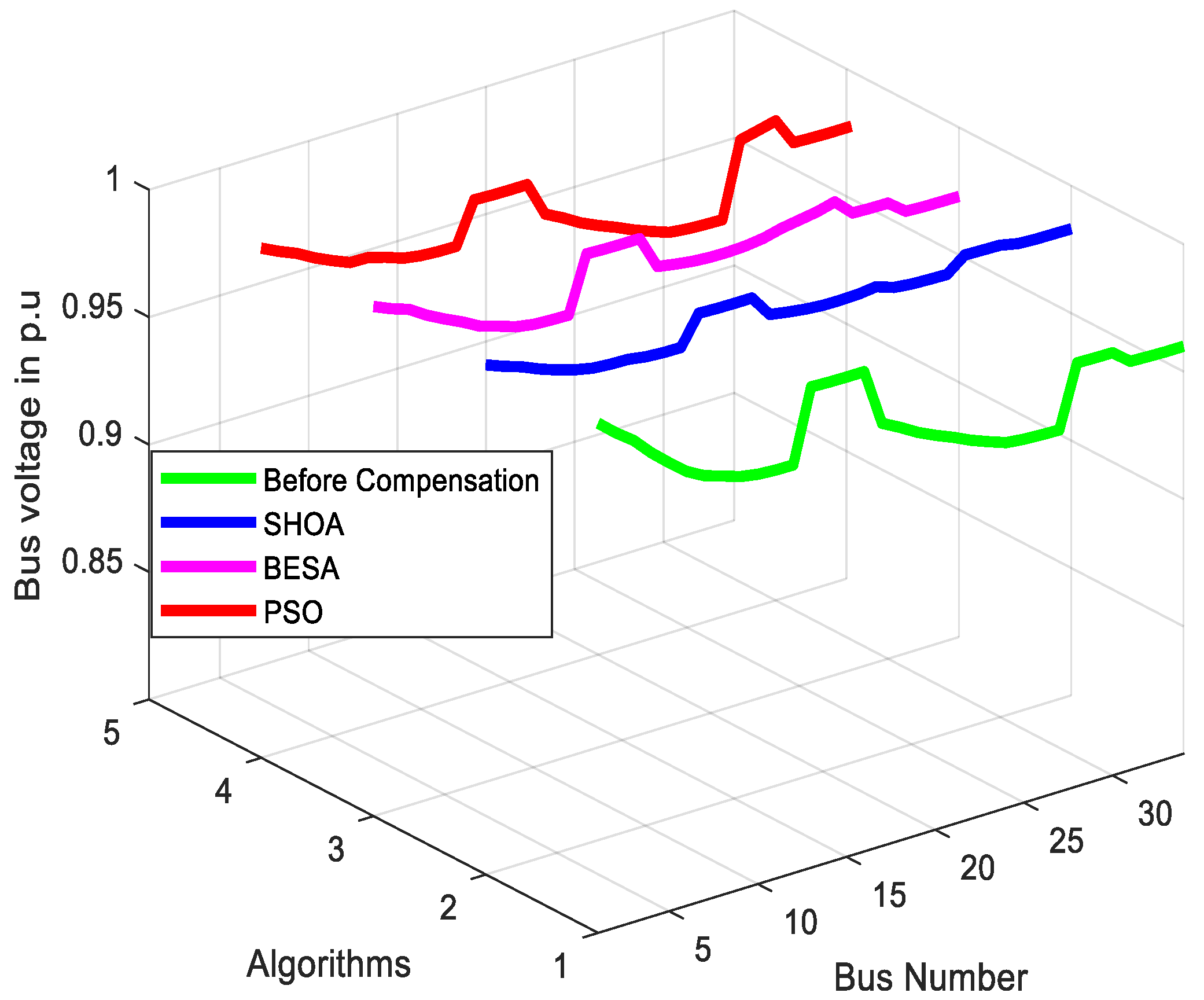
- (iv)
- Bus Voltage Improvement
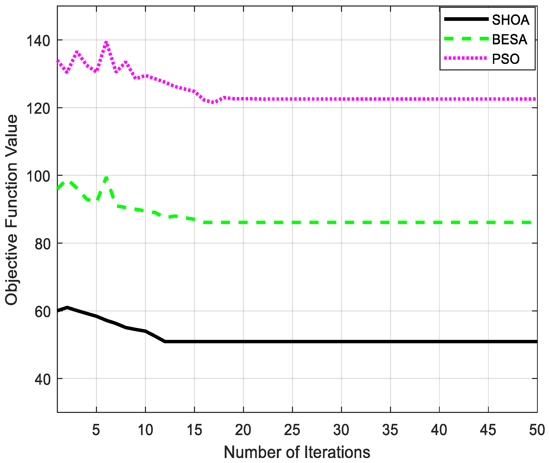
4.3. Comparative Analysis
5. Conclusions
Author Contributions
Funding
Institutional Review Board Statement
Informed Consent Statement
Data Availability Statement
Conflicts of Interest
References
- Zeb, M.Z.; Imran, K.; Khattak, A.; Janjua, A.K.; Pal, A.; Nadeem, M.; Zhang, J.; Khan, S. Optimal Placement of Electric Vehicle Charging Stations in the Active Distribution Network. IEEE Access 2020, 8, 68124–68134. [Google Scholar] [CrossRef]
- Alotaibi, I.; Abido, M.A.; Khalid, M.; Savkin, A.V. A comprehensive review of recent advances in smart grids: A sustainable future with renewable energy resources. Energies 2020, 13, 6269. [Google Scholar] [CrossRef]
- Kazemtarghi, A. Electric Vehicle Charging Systems: From Converter Level Optimization to Impact Analysis on Power Systems. Doctoral Dissertation, Arizona State University, Tempe, AZ, USA, 2024. [Google Scholar]
- FREI, A.A.M. Optimal Accommodation of DERs in Practical Radial Distribution Feeder for Techno-Economic and Environmental Benefits under Load Uncertainty Condition. Doctoral Dissertation, Karabuk University, Karabük, Türkiye, 2022. [Google Scholar]
- Un-Noor, F.; Padmanaban, S.; Mihet-Popa, L.; Mollah, M.N.; Hossain, E. A comprehensive study of key electric vehicle (EV) components, technologies, challenges, impacts, and future direction of development. Energies 2017, 10, 1217. [Google Scholar] [CrossRef]
- Rahman, S.; Khan, I.A.; Khan, A.A.; Mallik, A.; Nadeem, M.F. Comprehensive review & impact analysis of integrating projected electric vehicle charging load to the existing low voltage distribution system. Renew. Sustain. Energy Rev. 2022, 153, 111756. [Google Scholar]
- Tavakoli, A.; Saha, S.; Arif, M.T.; Haque, M.E.; Mendis, N.; Oo, A.M. Impacts of grid integration of solar PV and electric vehicle on grid stability, power quality and energy economics: A review. IET Energy Syst. Integr. 2020, 2, 243–260. [Google Scholar] [CrossRef]
- Omer, A.M. Energy use and environmental impacts: A general review. J. Renew. Sustain. Energy 2009, 1, 053101. [Google Scholar] [CrossRef]
- Bokopane, L.; Kusakana, K.; Vermaak, H.; Hohne, A. Optimal power dispatching for a grid-connected electric vehicle charging station microgrid with renewable energy, battery storage and peer-to-peer energy sharing. J. Energy Storage 2024, 96, 112435. [Google Scholar] [CrossRef]
- Suresh, M.P.; Yuvaraj, T.; Thanikanti, S.B.; Nwulu, N. Optimizing smart microgrid performance: Integrating solar generation and static VAR compensator for EV charging impact, emphasizing SCOPE index. Energy Rep. 2024, 11, 3224–3244. [Google Scholar] [CrossRef]
- Humfrey, H.; Sun, H.; Jiang, J. Dynamic charging of electric vehicles integrating renewable energy: A multi-objective optimisation problem. IET Smart Grid 2019, 2, 250–259. [Google Scholar] [CrossRef]
- Saw, B.K.; Bohre, A.K.; Jobanputra, J.H.; Kolhe, M.L. Solar-DG and DSTATCOM concurrent planning in reconfigured distribution system using APSO and GWO-PSO based on novel objective function. Energies 2022, 16, 263. [Google Scholar] [CrossRef]
- Lam, A.Y.; Leung, Y.W.; Chu, X. Electric vehicle charging station placement: Formulation, complexity, and solutions. IEEE Trans. Smart Grid 2014, 5, 2846–2856. [Google Scholar] [CrossRef]
- Anadón Martínez, V.; Sumper, A. Planning and operation objectives of public electric vehicle charging infrastructures: A review. Energies 2023, 16, 5431. [Google Scholar] [CrossRef]
- Ahmad, F.; Iqbal, A.; Ashraf, I.; Marzband, M.; Khan, I. The Optimal Placement of Electric Vehicle Fast Charging Stations in the Electrical Distribution System with Randomly Placed Solar Power Distributed Generations. Distrib. Gener. Altern. Energy J. 2022, 37, 1277–1304. [Google Scholar] [CrossRef]
- Deb, S.; Tammi, K.; Kalita, K.; Mahanta, P. Impact of electric vehicle charging station load on distribution network. Energies 2018, 11, 178. [Google Scholar] [CrossRef]
- Ahmad, F.; Iqbal, A.; Asharf, I.; Marzband, M.; Khan, I. Placement and capacity of ev charging stations by considering uncertainties with energy management strategies. IEEE Trans. Ind. Appl. 2023, 59, 3865–3874. [Google Scholar] [CrossRef]
- Bilal, M.; Rizwan, M. Integration of electric vehicle charging stations and capacitors in distribution systems with vehicle-to-grid facility. Energy Sources Part A Recovery Util. Environ. Eff. 2021, 1–30. [Google Scholar] [CrossRef]
- Huiling, T.; Jiekang, W.; Fan, W.; Lingmin, C.; Zhijun, L.; Haoran, Y. An optimization framework for collaborative control of power loss and voltage in distribution systems with DGs and EVs using stochastic fuzzy chance constrained programming. IEEE Access 2020, 8, 49013–49027. [Google Scholar] [CrossRef]
- Wu, J.; Wu, Z.; Wu, F.; Tang, H.; Mao, X. CVaR risk-based optimization framework for renewable energy management in distribution systems with DGs and EVs. Energy 2018, 143, 323–336. [Google Scholar] [CrossRef]
- Shaaban, M.F.; Mohamed, S.; Ismail, M.; Qaraqe, K.A.; Serpedin, E. Joint planning of smart EV charging stations and DGs in eco-friendly remote hybrid microgrids. IEEE Trans. Smart Grid 2019, 10, 5819–5830. [Google Scholar] [CrossRef]
- Muthukannan, S.; Karthikaikannan, D. Multiobjective planning strategy for the placement of electric-vehicle charging stations using hybrid optimization algorithm. IEEE Access 2022, 10, 48088–48101. [Google Scholar] [CrossRef]
- Ahmad, F.; Ashraf, I.; Iqbal, A.; Khan, I.; Marzband, M. Optimal location and energy management strategy for EV fast charging station with integration of renewable energy sources. In Proceedings of the 2022 IEEE Silchar Subsection Conference (SILCON), Silchar, India, 4–6 November 2022; IEEE: Piscataway, NJ, USA, 2022; pp. 1–6. [Google Scholar]
- Mohanty, A.K.; Babu, P.S.; Salkuti, S.R. Fuzzy-based simultaneous optimal placement of electric vehicle charging stations, distributed generators, and DSTATCOM in a distribution system. Energies 2022, 15, 8702. [Google Scholar] [CrossRef]
- Erdinc, O.; Tascikaraoglu, A.; Paterakis, N.G.; Dursun, I.; Sinim, M.C.; Catalao, J.P.S. Comprehensive optimization model for sizing and siting of DG units, EV charging stations, and energy storage systems. IEEE Trans. Smart Grid 2017, 9, 3871–3882. [Google Scholar] [CrossRef]
- Gurappa, B.; Yammani, C.; Maheswarapu, S. Multi-objective simultaneous optimal planning of electrical vehicle fast charging stations and DGs in distribution system. J. Mod. Power Syst. Clean Energy 2019, 7, 923–934. [Google Scholar]
- Pratap, A.; Tiwari, P.; Maurya, R.; Singh, B. Minimisation of electric vehicle charging stations impact on radial distribution networks by optimal allocation of DSTATCOM and DG using African vulture optimisation algorithm. Int. J. Ambient. Energy 2022, 43, 8653–8672. [Google Scholar] [CrossRef]
- Sadeghi, D.; Amiri, N.; Marzband, M.; Abusorrah, A.; Sedraoui, K. Optimal sizing of hybrid renewable energy systems by considering power sharing and electric vehicles. Int. J. Energy Res. 2022, 46, 8288–8312. [Google Scholar] [CrossRef]
- Khan, M.O.; Kirmani, S.; Rihan, M.; Pandey, A.K. Stochastic Modelling and Integration of Electric Vehicles in the Distribution System Using the Jaya Algorithm. IETE J. Res. 2024, 1–16. [Google Scholar] [CrossRef]
- Jabari, F.; Sohrabi, F.; Pourghasem, P.; Mohammadi-Ivatloo, B. Backward-forward sweep based power flow algorithm in distribution systems. In Optimization of Power System Problems: Methods, Algorithms and MATLAB Codes; Springer: Cham, Switzerland, 2020; pp. 365–382. [Google Scholar]
- Chakravorty, M.; Das, D. Voltage stability analysis of radial distribution networks. Int. J. Electr. Power Energy Syst. 2001, 23, 129–135. [Google Scholar] [CrossRef]
- Kayal, P.; Chanda, C. Placement of wind and solar based DGs in distribution system for power loss minimization and voltage stability improvement. Int. J. Electr. Power Energy Syst. 2013, 53, 795–809. [Google Scholar] [CrossRef]
- Yuvaraj, T.; Krishnamoorthy, R.; Arun, S.; Thanikanti, S.B.; Nwulu, N. Optimizing virtual power plant allocation for enhanced resilience in smart microgrids under severe fault conditions using the hunting prey optimization algorithm. Energy Rep. 2024, 11, 6094–6108. [Google Scholar] [CrossRef]
- International Energy Agency (IEA). Global EV Outlook 2022; International Energy Agency: Paris, France, 2022. [Google Scholar]
- U.S. Department of Energy (DOE). Electric Vehicle Battery Costs and Other Factors Affecting EVs; Office of Energy Efficiency & Renewable Energy: Washington, DC, USA, 2023. [Google Scholar]
- IEA. Charging Infrastructure for Electric Vehicles; International Energy Agency: Paris, France, 2023. [Google Scholar]
- Mustafa, M.; Anandhakumar, G.; Jacob, A.A.; Singh, N.P.; Asha, S.; Jayadhas, S.A. Hybrid renewable power generation for modeling and controlling the battery storage photovoltaic system. Int. J. Photoenergy 2022, 2022, 9491808. [Google Scholar] [CrossRef]
- Dhiman, G.; Kumar, V. Spotted hyena optimizer: A novel bio-inspired based metaheuristic technique for engineering applications. Adv. Eng. Softw. 2017, 114, 48–70. [Google Scholar] [CrossRef]
- Montoya, O.D.; Molina-Cabrera, A.; Hernández, J.C. A comparative study on power flow methods applied to AC distribution networks with single-phase representation. Electronics 2021, 10, 2573. [Google Scholar] [CrossRef]
- Alsattar, H.A.; Zaidan, A.A.; Zaidan, B.B. Novel meta-heuristic bald eagle search optimisation algorithm. Artif. Intell. Rev. 2020, 53, 2237–2264. [Google Scholar] [CrossRef]
- Kennedy, J.; Eberhart, R. 1995Particle swarm optimization. In Proceedings of the ICNN’95-International Conference on Neural Networks, Perth, WA, Australia, 27 November–1 December 1995; IEEE: Piscataway, NJ, USA, 1995; Volume 4, pp. 1942–1948. [Google Scholar]


| Ref. No. | Dynamic Analysis | EVCS | G2V Mode | V2G Mode | RDG | DSTATCOM | Objective Function | Test System | Techniques |
|---|---|---|---|---|---|---|---|---|---|
| [15] | × | √ | √ | × | √ | × | Power loss | IEEE 34-bus | IBESA |
| [16] | × | √ | √ | × | × | × | MOF | IEEE 33-bus | VRP Index |
| [17] | √ | √ | √ | √ | √ | × | MOF | IEEE 33-bus | MCS method |
| [18] | × | √ | √ | √ | × | × | MOF | IEEE 33- & 34-bus | Hybrid GWO & PSO |
| [19] | √ | √ | √ | × | √ | × | MOF | IEEE 33- & 118-bus | Stochastic Fuzzy |
| [20] | √ | √ | √ | × | √ | × | Power loss | IEEE 69-bus | CCSOCP |
| [21] | × | √ | √ | × | √ | × | MOF | Hybrid AC/DC 38-bus | JPA |
| [22] | × | √ | √ | × | × | × | MOF | IEEE 33- & 69-bus | PSO |
| [23] | × | √ | √ | × | √ | × | MOF | IEEE 33-bus | IBESA |
| [24] | × | √ | √ | × | × | √ | Power loss | Indian 28- & 108-bus | BESA |
| [25] | √ | √ | √ | × | √ | × | MOF | Real Istanbul buses | MOSEK |
| [26] | √ | √ | √ | × | √ | × | MOF | IEEE 118-bus | MINLP |
| [27] | × | √ | √ | × | × | √ | MOF | IEEE 33-, 69- & 136-bus | AVOA |
| [28] | √ | √ | √ | × | √ | × | MOF | Distribution systems | MOPSO & MOCS |
| [29] | × | √ | √ | √ | √ | × | MOF | IEEE 33- & 69-bus | Jaya algorithm |
| Proposed Method | √ | √ | √ | √ | √ | √ | Power loss | IEEE 34-bus | SHOA |
| Time in Hours | Real Power Loss in kW | Reactive Power Loss in kVAr | VSI in p.u. | Bus Voltage in p.u. | ||||
|---|---|---|---|---|---|---|---|---|
| Before | After | Before | After | Before | After | Before | After | |
| 1 | 165.37 | 80.09 | 48.66 | 22.33 | 0.8143 | 0.9109 | 0.9499 | 0.9769 |
| 2 | 157.55 | 76.37 | 46.36 | 21.25 | 0.8184 | 0.9138 | 0.9511 | 0.9777 |
| 3 | 153.72 | 74.14 | 45.23 | 20.63 | 0.8205 | 0.9149 | 0.9517 | 0.978 |
| 4 | 149.94 | 72.76 | 44.12 | 20.16 | 0.8226 | 0.9167 | 0.9523 | 0.9785 |
| 5 | 149.94 | 72.62 | 44.12 | 20.08 | 0.8226 | 0.9171 | 0.9523 | 0.9786 |
| 6 | 161.44 | 76.76 | 47.5 | 21.27 | 0.8164 | 0.9151 | 0.9505 | 0.9781 |
| 7 | 173.4 | 62.1 | 51.02 | 16.97 | 0.8102 | 0.9258 | 0.9487 | 0.9809 |
| 8 | 190.07 | 71.91 | 55.92 | 20.27 | 0.8019 | 0.9118 | 0.9463 | 0.9771 |
| 9 | 190.07 | 65.59 | 55.92 | 18.71 | 0.8019 | 0.9065 | 0.9463 | 0.9757 |
| 10 | 194.37 | 61.39 | 57.18 | 17.52 | 0.7999 | 0.9062 | 0.9457 | 0.9756 |
| 11 | 194.37 | 56.34 | 57.18 | 15.87 | 0.7999 | 0.9146 | 0.9457 | 0.9779 |
| 12 | 190.07 | 43.18 | 55.92 | 11.6 | 0.8019 | 0.9457 | 0.9463 | 0.9863 |
| 13 | 181.63 | 42.79 | 53.44 | 10.99 | 0.806 | 0.9537 | 0.9475 | 0.9882 |
| 14 | 177.49 | 44.5 | 52.22 | 11.3 | 0.8081 | 0.9531 | 0.9481 | 0.9881 |
| 15 | 181.63 | 51.18 | 53.44 | 12.84 | 0.806 | 0.9495 | 0.9475 | 0.9871 |
| 16 | 181.63 | 56.51 | 53.44 | 14.24 | 0.806 | 0.9424 | 0.9475 | 0.9853 |
| 17 | 185.83 | 64.32 | 54.67 | 16.22 | 0.804 | 0.935 | 0.9469 | 0.9833 |
| 18 | 185.83 | 83.81 | 54.67 | 22.83 | 0.804 | 0.9164 | 0.9469 | 0.9784 |
| 19 | 221.28 | 107.88 | 65.09 | 30.36 | 0.7875 | 0.8903 | 0.942 | 0.9713 |
| 20 | 221.28 | 109.9 | 65.09 | 31.13 | 0.7875 | 0.8841 | 0.942 | 0.9696 |
| 21 | 203.13 | 100.47 | 59.76 | 28.3 | 0.7957 | 0.8931 | 0.9444 | 0.9721 |
| 22 | 181.63 | 88.9 | 53.44 | 24.88 | 0.806 | 0.9036 | 0.9475 | 0.9749 |
| 23 | 173.4 | 84.89 | 51.02 | 23.74 | 0.8102 | 0.9061 | 0.9487 | 0.9756 |
| 24 | 165.37 | 80.57 | 48.66 | 22.54 | 0.8143 | 0.9084 | 0.9499 | 0.9762 |
| Average | 180.43 | 72.04 | 53.08 | 19.83 | 0.8069 | 0.9181 | 0.9477 | 0.9788 |
| Time in Hours | Load Factor in p.u. | RDG Output in kW | DSTATCOM Output in kVAr | ||
|---|---|---|---|---|---|
| 9th Location (PV) | 23rd Location (WT) | 9th Location | 23rd Location | ||
| 1 | 0.87 | 0 | 1185 | 850 | 1050 |
| 2 | 0.85 | 0 | 1170 | 828 | 1040 |
| 3 | 0.84 | 0 | 1155 | 818 | 1026 |
| 4 | 0.83 | 0 | 1185 | 808 | 1015 |
| 5 | 0.83 | 0 | 1200 | 808 | 1015 |
| 6 | 0.86 | 30 | 1215 | 838 | 1050 |
| 7 | 0.89 | 200 | 1185 | 867 | 1088 |
| 8 | 0.93 | 400 | 1020 | 907 | 1137 |
| 9 | 0.93 | 700 | 900 | 907 | 1137 |
| 10 | 0.94 | 880 | 870 | 917 | 1150 |
| 11 | 0.94 | 980 | 945 | 917 | 1150 |
| 12 | 0.93 | 1000 | 1065 | 907 | 1137 |
| 13 | 0.91 | 970 | 1230 | 887 | 1113 |
| 14 | 0.9 | 860 | 1290 | 877 | 1100 |
| 15 | 0.91 | 700 | 1410 | 887 | 1113 |
| 16 | 0.91 | 450 | 1440 | 887 | 1113 |
| 17 | 0.92 | 240 | 1500 | 895 | 1125 |
| 18 | 0.92 | 80 | 1410 | 895 | 1125 |
| 19 | 1 | 0 | 1230 | 987 | 1200 |
| 20 | 1 | 0 | 1155 | 987 | 1200 |
| 21 | 0.96 | 0 | 1170 | 937 | 1174 |
| 22 | 0.91 | 0 | 1185 | 887 | 1113 |
| 23 | 0.89 | 0 | 1170 | 867 | 1088 |
| 24 | 0.87 | 0 | 1155 | 850 | 1050 |
| Time in Hours | PV-Based EVCS in kW | EVCS Mode | No. of EVs Connected to EVCS | ||
|---|---|---|---|---|---|
| EV Rating-7.4 kW | EV Rating-22 kW | EV Rating-350 kW | |||
| 1 | 0 | Idle | 0 | 0 | 0 |
| 2 | 0 | Idle | 0 | 0 | 0 |
| 3 | 0 | Idle | 0 | 0 | 0 |
| 4 | 0 | Idle | 0 | 0 | 0 |
| 5 | 0 | Idle | 0 | 0 | 0 |
| 6 | 0 | Idle | 0 | 0 | 0 |
| 7 | 0 | Idle | 0 | 0 | 0 |
| 8 | 225 | G2V | 34 | 11 | 0 |
| 9 | 315 | G2V | 47 | 15 | 1 |
| 10 | 315 | G2V | 47 | 15 | 1 |
| 11 | 315 | G2V | 47 | 15 | 1 |
| 12 | 315 | G2V | 47 | 15 | 1 |
| 13 | 306 | G2V | 46 | 15 | 1 |
| 14 | 270 | G2V | 41 | 13 | 0 |
| 15 | 225 | G2V | 34 | 11 | 0 |
| 16 | 135 | G2V | 20 | 6 | 0 |
| 17 | 81 | G2V | 12 | 4 | 0 |
| 18 | 24 | V2G | 0 | 0 | 0 |
| 19 | 0 | V2G | 0 | 0 | 0 |
| 20 | 0 | V2G | 0 | 0 | 0 |
| 21 | 0 | V2G | 0 | 0 | 0 |
| 22 | 0 | V2G | 0 | 0 | 0 |
| 23 | 0 | V2G | 0 | 0 | 0 |
| 24 | 0 | Idle | 0 | 0 | 0 |
| Time in Hours | WT-Based EVCS in kW | EVCS Mode | No. of EVs Connected to EVCS | ||
|---|---|---|---|---|---|
| EV Rating-7.4 kW | EV Rating-22 kW | EV Rating-350 kW | |||
| 1 | 315 | G2V | 47 | 15 | 1 |
| 2 | 306 | G2V | 46 | 15 | 1 |
| 3 | 297 | G2V | 45 | 15 | 1 |
| 4 | 315 | G2V | 47 | 15 | 1 |
| 5 | 315 | G2V | 48 | 16 | 1 |
| 6 | 315 | G2V | 49 | 16 | 1 |
| 7 | 0 | Idle | 0 | 0 | 0 |
| 8 | 0 | Idle | 0 | 0 | 0 |
| 9 | 0 | Idle | 0 | 0 | 0 |
| 10 | 0 | Idle | 0 | 0 | 0 |
| 11 | 0 | Idle | 0 | 0 | 0 |
| 12 | 280 | V2G | 47 | 15 | 1 |
| 13 | 280 | V2G | 47 | 15 | 1 |
| 14 | 280 | V2G | 49 | 16 | 1 |
| 15 | 280 | V2G | 57 | 17 | 1 |
| 16 | 280 | V2G | 59 | 18 | 1 |
| 17 | 280 | V2G | 61 | 19 | 1 |
| 18 | 315 | G2V | 57 | 17 | 1 |
| 19 | 315 | G2V | 47 | 15 | 1 |
| 20 | 315 | G2V | 47 | 15 | 1 |
| 21 | 315 | G2V | 47 | 15 | 1 |
| 22 | 315 | G2V | 47 | 15 | 1 |
| 23 | 315 | G2V | 47 | 15 | 1 |
| 24 | 315 | G2V | 47 | 15 | 1 |
| Items | Before Compensation | After Compensation | ||
|---|---|---|---|---|
| SHOA | BESA [40] | PSO [41] | ||
| Location & Capacity of EVCS (G2V) in kW | Not Available | 287 (9) | 328 (13) | 339 (6) |
| Location & Capacity of EVCS (V2G) in kW | Not Available | 220 (23) | 310 (27) | 208 (30) |
| Location & Capacity of PV in kW | Not Available | 980 (9) | 859 (13) | 790 (6) |
| Location & Capacity of WT in kW | Not Available | 1020 (23) | 989 (27) | 880 (30) |
| Location & Capacity of DSTATCOM in kVAr | Not Available | 890 (9) 1000 (23) | 730 (13) 870 (27) | 630 (6) 780 (30) |
| in kW | 221.29 | 50.91 | 86.14 | 122.53 |
| in kVAr | 65.09 | 14.38 | 22.22 | 31.92 |
| in p.u. | 0.7875 | 0.9228 | 0.8960 | 0.8348 |
| in p.u. | 0.9420 | 0.9801 | 0.9729 | 0.9558 |
| Convergence Time (s) | -- | 8.86 | 10.52 | 14.06 |
Disclaimer/Publisher’s Note: The statements, opinions and data contained in all publications are solely those of the individual author(s) and contributor(s) and not of MDPI and/or the editor(s). MDPI and/or the editor(s) disclaim responsibility for any injury to people or property resulting from any ideas, methods, instructions or products referred to in the content. |
© 2024 by the authors. Licensee MDPI, Basel, Switzerland. This article is an open access article distributed under the terms and conditions of the Creative Commons Attribution (CC BY) license (https://creativecommons.org/licenses/by/4.0/).
Share and Cite
Yuvaraj, T.; Prabaharan, N.; John De Britto, C.; Thirumalai, M.; Salem, M.; Nazari, M.A. Dynamic Optimization and Placement of Renewable Generators and Compensators to Mitigate Electric Vehicle Charging Station Impacts Using the Spotted Hyena Optimization Algorithm. Sustainability 2024, 16, 8458. https://doi.org/10.3390/su16198458
Yuvaraj T, Prabaharan N, John De Britto C, Thirumalai M, Salem M, Nazari MA. Dynamic Optimization and Placement of Renewable Generators and Compensators to Mitigate Electric Vehicle Charging Station Impacts Using the Spotted Hyena Optimization Algorithm. Sustainability. 2024; 16(19):8458. https://doi.org/10.3390/su16198458
Chicago/Turabian StyleYuvaraj, Thangaraj, Natarajan Prabaharan, Chinnappan John De Britto, Muthusamy Thirumalai, Mohamed Salem, and Mohammad Alhuyi Nazari. 2024. "Dynamic Optimization and Placement of Renewable Generators and Compensators to Mitigate Electric Vehicle Charging Station Impacts Using the Spotted Hyena Optimization Algorithm" Sustainability 16, no. 19: 8458. https://doi.org/10.3390/su16198458
APA StyleYuvaraj, T., Prabaharan, N., John De Britto, C., Thirumalai, M., Salem, M., & Nazari, M. A. (2024). Dynamic Optimization and Placement of Renewable Generators and Compensators to Mitigate Electric Vehicle Charging Station Impacts Using the Spotted Hyena Optimization Algorithm. Sustainability, 16(19), 8458. https://doi.org/10.3390/su16198458