An Efficient Computational Analysis and Modelling of Transferred Aerodynamic Loading on Direct-Drive System of 5 MW Wind Turbine and Results Driven Optimisation for a Sustainable Generator Structure

Abstract

The study presents an efficient computational investigation on the behaviour of the direct-drive system integrated into the offshore 5 MW NREL wind turbine model under demanding aerodynamic loading conditions with the aim of optimising and developing more sustainable key structural components. The research was based on computational simulation packages in order to verify the use of real-world wind data and the loading conditions on the blade structures through aero-elastic simulation studies as well as analyse the behaviour of the drive system. Through the application of validated aerodynamic loading conditions, resulting normal forces on the blades structure were obtained and applied to a dedicated simplified model that was also previously validated to estimate the transferred loads into the powertrain. The adopted methodology allowed for the identification of shaft misalignment induced air gap eccentricity. The impact of shaft deflections on resulting magnetomotive force was considered by making use of the Maxwell stress distribution expression. By taking into account the resulting loading cases on the generator structure, as well as the inherent typical loads generated by the electrical machine, a procedure including structural parametric and topology optimisation was developed and performed, achieving a rotor mass reduction between 8.5 and 9.6% compared to the original model.

1. Introduction

Renewable energy sources have grasped the attention of the media and the public in recent years. This is mainly due to the prospect of decarbonising the economy, tackling the ever-growing climate change issue, and supporting the idea of a sustainable future. With increased popularity, the electricity generation from wind power in the UK has increased by 715% from 2009 to 2020, resulting in a turnover of nearly £6 billion in 2019 [1]. With planned investments regarding the installation of offshore wind turbines and Europe’s predictions reaching 85 GW in the Baltic Sea alone, the need for well-designed and optimised turbines is significant [2].

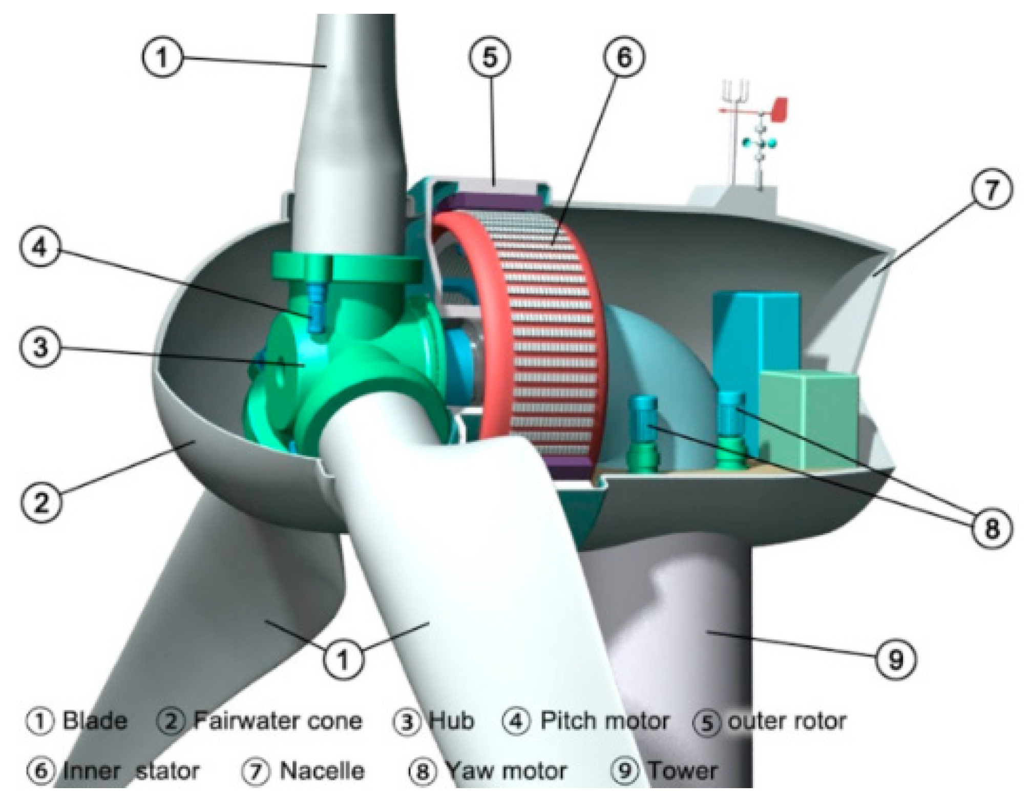
The following investigation presents a study on the 5 MW reference direct-driven wind turbine designed by the National Renewable Energy Laboratory (NREL). This model is a benchmark structure for the majority of the conducted academic investigations towards improvement of the structure. Large horizontal axis wind turbines can be divided into gearbox-driven and direct-driven turbines. Typically, gearbox-driven wind turbines are designed to transfer the mechanical energy from a low-rotational-speed rotor to a double-fed induction generator with high rotational speed. Direct-driven wind turbines (Figure 1) have a rotor directly coupled to a permanent magnet synchronous generator, omitting additional components required for the change of rotational speed via gear ratio [3]. Ultimately the elimination of additional components simplifies the structure and limits the probability of standard gearbox failures, as well as the costs associated with these occurrences. However, the heavier rotor system in direct-drive turbines results in higher loads on supporting structures such as bearings.

Mass optimisation of direct drive electrical generator wind turbines’ structures became a crucial study area. It results in lower maintenance and handling costs and more sustainable systems, which can also be suitable for other applications, as described by the authors in [5]. It has been stated that the total inactive mass (supporting structures) of rotor and stator structures share up to 82% of total mass for a 5 MW turbine [6].

The main components of the generator structure are presented in Figure 2. The blades of the wind turbine generate mechanical rotation by capturing the kinetic energy of the wind. This motion energy is then transferred by the shaft to the rotor. This results in a spinning motion of the rotor inside the stator structure. The rotor and stator are separated from each other by a fixed distance called an air gap. Moreover, the stator is fitted with strong magnets, whereas the rotor accommodates coils of wire. Ultimately, a changing magnetic field is introduced to the system by the spinning magnets, thus inducing an electrical current through electromagnetic induction. Further instrumentation within the nacelle converts the current into a more stable form of electricity.

An in-depth investigation of the loads and structural integrity of the machinery is essential in order to enable any optimisation attempts without compromising model reliability. Typically, the loading conditions consist of the magnetic attraction of the moving parts and the previously mentioned stationary components of the generator, shear loading, gravitational loading due to the weight of the structure, thermal expansion of the generator structure, and centrifugal loading. The representation of these loads can be seen in Figure 3.

Furthermore, when looking at the behaviour of the rotor, it is essential to understand how the structure can deflect under loading conditions. Four modes of deflection were presented in Figure 4. In Mode 0, the rotor will deflect in a uniform manner in the radial direction. In case of a local deformation, frequently caused by the shaft misalignment in the system, the structure will experience mode 1 deflection. For mode 2, the structure tends to ovalise, whereas in mode 3, the structure will deflect following the pattern of ripples.

Shaft misalignment can be one of the main contributors to nonuniformity of the air gap in the stator and rotor system. This can result in an unbalanced magnetic pull, ultimately disturbing the equilibrium of the magnetic attraction forces, which results in a dynamic radial load on the bearings, undesirable noise, and vibration due to the increase in space harmonics [8]. Therefore, it is essential to carry out numerical simulations of the drivetrain to correctly predict the behavioural response of the analysed system. An air gap in wind turbines refers to the distance between the rotor and stator of the generator. The rotor is the part of the wind turbine that rotates and contains the magnets, while the stator is stationary and contains the teeth and wire coils that transfer the electricity to the grid going through the converter first.

Due to the rotational movement depicted in Figure 5, magnetic and gravitational forces are present at the rotor. Therefore, the structure will experience deformation. Consequently, the air gap will be reduced. This phenomenon will be further magnified by the recognised shaft misalignment caused by aerodynamic loading. Additional forces in five degrees of freedom, as well as forces caused by thermal expansion and shear, can be identified. However, they were deemed negligible for the purpose of this study. The allowable resultant air gap deflection is stated to be 10–20% for direct-drive structures. This limit ensures that the air gap flux density will not increase to dangerous levels that can produce the collapse of the machine [8,9].

In order to conduct viable simulations on the wind turbine structure and obtain the loads present, wind data must be collected. According to IEC 61400-50:2022 “Wind measurement—Overview” [10], all data will be typically reduced to 10-min statistics (mean, minimum, maximum, standard deviation) for use as input for analysis. Wind measurements are made more detailed and accurate by the use of remote sensing devices (RSDs) such as lidars and sodars. They are more reliable than cup anemometers since they provide full three-dimensional wind measurements and are not influenced by mechanical limitations due to environmental conditions (humidity, temperature, icing). IEC 61400-50 series of standards specify requirements and methods for the use, calibration and classification of conventional cup anemometers, whereas standardized ultrasonic anemometers must be compliant with the rules [10].

The proposed approach in this study indicates that the loading conditions, stresses, and behavioural shaft response can be obtained through the application of real-world data sets after appropriate site selection and analysis. Moreover, by referencing technical reports on 5 MW NREL reference wind turbine [11], a simplified assembly CAD model can be produced, which can significantly reduce the computing time and is valid for conducting structural optimisations leading to more sustainable systems.

2. Methodology

In this study, the authors present a novel procedure for developing and validating an efficient computational model that can be analysed and employed to optimise multi-MW electrical generator rotor supporting structures usingthe most structurally significant variables. Currently, models used by the industry for the design of electrical machines do not consider the external loading conditions related to the operation of the wind turbine rotor. With the use of this model and following the proposed methodology, one can reduce the amount of material needed to withstand the demanding loading conditions, which include not only the typically considered inherent generator operation loads but also the external conditions. The consideration of the mentioned external loading conditions is of significant importance, as the displacements experienced by the electrical generator rotor—which in turn produce changes in the air gap length and generate variations in the electromagnetic flux, leading to peaks in the induced voltages and increments in temperature—play an important role when estimating the remaining life of the machine and its maintenance procedures. Looking at this issue in greater detail, it is worth mentioning that those rises in temperature have a considerable effect on the lifespan of the winding insulation system. Loss of insulation in the winding has been clearly identified as the main aspect related to early failures of electrical generators by other researchers, as specified in Section 3. High benefits in terms of downtime reduction, cost savings and factor have been estimated if this issue can be somehow mitigated or fully eliminated. An integrated model that considers the manufacturing, labour, installation, and transportation time as well as the associated resources that can be diminished with the consequent reductions in CO₂ and methane emissions, water usage, and costs is another contribution made by this investigation. The effect of those modifications can be quantified by looking at the changes in the structure’s natural frequencies and the impact in the generator’s operating range and turbine’s energy-harvesting capability. Lastly, the computational sustainability was taken into account by finding the optimum number of simulations required to produce meaningful data without compromising the accuracy of the results.

The methodology of the conducted research can be found in Figure 6. Firstly, real-world wind datasets were obtained and selected after careful investigation and appraisal of the corresponding wind farms. The chosen data package was then further analysed and edited. This resulted in the creation of three aerodynamic settings corresponding to the considered wind speeds: Low, Rated and High. Moreover, the wind patterns at the chosen site were specified. The obtained data was validated through a correlation study of wind speeds and corresponding altitudes. To translate the real-world wind behaviour to software-aided analysis, windfield simulations in QBlade (CE v 2.0.4.8) were conducted. The obtained results were compared against real-world data. Subsequently, the validated windfield data were used in dynamic, structural simulations on a 5 MW wind turbine in QBlade. Thus, output values for normal stresses on the blades were acquired. Following the analysis of the wind turbine in QBlade, a simplified drivetrain system was created. Finite element analysis of the system was conducted after the simulation set-up procedure in Solidworks, which consisted of material properties specification, application of fixtures, and mesh independence study. The results were then validated through comparative investigation between the gathered data from QBlade and Solidworks. Furthermore, the shaft misalignment induced eccentricity in relation to the air gap of the concentric rotor was calculated for the Rated and High aerodynamic settings. The resultant shaft deflections were included in the rotor optimisation procedure, which consisted of rotor structural configuration selection, static FE analysis, topology optimisation, parametric table optimisation, and modal analysis of the optimised structures. Lastly, the environmental impact and sustainability of the proposed designs and procedures were studied.

2.1. Wind Data Analysis

A total of three different wind data sets from wind farm sites—Penmanshiel, Anholt, and Westermost Rough—were found and taken into account. The Penmanshiel wind farm dataset was obtained from the online repository Zenodo [12] released by Cubico Sustainable Investments Ltd., London, UK [13], whereas the Anholt and Westermost Rough wind farm datasets were supplied by Ørsted, Fredericia, Denmark [14]. The chosen data sets for this study came from Anholt wind farm located in eastern Denmark. They were found suitable, as they cover the measurement height requirement for further studies and come with already transposed values e.g., wind direction, thus reducing the workload during the analysis. The technical data and location for Anholt site is provided in

Table 1. Anholt wind farm technical data.

Latitude	56°35′44.4″ N
Longitude	11°09′09.8″ E
No. of Turbines	111
Total Nominal Power	400 MW
Turbine Nominal Power	3.6 MW
Turbine Rotor Diameter	120 m
Location	Offshore
Status *	Operational

* as of 10 September 2023.

.

The overall wind turbine power is smaller than the investigated structure in this study. However, the data provided from this site covers a range of altitudes for even the biggest commercially used structures at the time (up to 315.6 m above lowest astronomical tide). Therefore, the wind data are only dependent on the environmental conditions present at the site. The data sets from the Anholt wind farm were found to be suitable for further analysis and validation. The obtained data package consists of various signals produced by continuous measurements in 10-min intervals taken at the site over 726 days, which totals to approximately 2 years and ultimately produced over 100,000 data rows and 150 columns. The columns specify the type of measurement taken over the period and consist of wind speed values, wind directions, and 12 different corresponding altitudes. The first 10 altitudes (65.6–315.6 m) were taken into consideration, as those heights would cover the operational area of the studied wind turbine.

Having a significant amount of data measured over a 2-year period, wind direction probability can be identified to analyse the working environment of wind turbine while operating. Firstly, the wind data for wind directions and wind speeds was limited to only one column set corresponding to closest hub-height altitude of 5 MW wind turbine—altitude 2. The chosen data were then sorted according to wind direction in 22.5° increments, ultimately resulting in a specified data set with identified 16 cardinal directions. The wind speeds were then divided into nine categories corresponding to the chosen values, sorted, and counted in Excel in order to produce a clear probability table that refers to the wind speed and wind direction values over the measurement period—2 years. The data can be presented as a wind rose (Figure 7) for better presentation of the results.

The chosen wind speeds were colour-coded. The graphed areas correspond to the wind direction as well as probability of occurrence at Anholt wind farm. The highest probability of 10% occurs at SSW direction for four wind speed categories with values over 17 $\mathrm{m}/\mathrm{s}$. The overall probability of the wind speed being over 5 $\mathrm{m}/\mathrm{s}$ is 89.55% and 69% for speeds over 8 $\mathrm{m}/\mathrm{s}$. Moreover, a recommended annual wind speed average for utility-scale wind turbines is at least 5.8 $\mathrm{m}/\mathrm{s}$. The average wind speed at Anholt wind farm is 10.83 $\mathrm{m}/\mathrm{s}$, which validates the site’s operational requirements.

In order to conduct further analysis, three wind speed scenarios were created—Low, Rated, and High—which respectively correspond to the lowest possible operational wind speed of 3 $\mathrm{m}/\mathrm{s}$ (cut-in speed), a rated wind speed of 11.4 $\mathrm{m}/\mathrm{s}$, and the highest possible operational wind speed 25 $\mathrm{m}/\mathrm{s}$ (cut-off speed) for a 5 MW wind turbine, respectively. For the purposes of data filtering, the three settings were given a range of wind speed values of 1 $\mathrm{m}/\mathrm{s}$. For Low and High settings, the lowest and highest possible operational wind speeds (cut-in/cut-off) were the boundaries, respectively. Whereas, for a rated wind speed of 11.4 $\mathrm{m}/\mathrm{s}$, the boundaries were set to ±0.5 $\mathrm{m}/\mathrm{s}$. This results in higher data count that is centralised about the specified value for each of the settings. As previously mentioned, the data were filtered against the closest altitude to the hub height (90 m) of the 5 MW WT.

The average wind speeds were then calculated for each of the 3 settings for 10 predetermined altitudes. The obtained results followed a normalised pattern with coefficient of determination R² of over 0.94, which shows a good correlation of the data and minimum impact of the irregularities. The exemplary correlation graph for Rated wind speed can be seen in Figure 8.

2.2. Windfield Simulations and Validation

With the average wind speeds found at specified altitudes, further validation study can be conducted. By using the QBlade simulation software, it is possible to create a windfield—a three-dimensional spatial pattern of winds—which will be used in the following structural simulations as an aerodynamic load on blades. However, firstly, the already verified Anholt wind farm data needed to be compared to the software’s output data in order to correlate and validate the two sources of data against each other. For this purpose, the wind speeds for Low, Rated, and High settings were recreated in the software and compared to the real-world data. The simulated windfields can be shown as three-dimensional graphs, and an example of an output graph can be seen in Figure 9a,b. The windfield changes over time of the simulation, acting like a turbulent model and mimicking the natural flow.

Using the export function of the software, it is possible to obtain exact values at particular points of the windfield. Therefore, after setting up the control points (wind probes) at heights corresponding to the measurement altitudes at Anholt wind farm, new data sets have been obtained. The results for Low-, Rated-, and High-setting windfields (simulated data) were obtained through a setup of 10 wind probes, data export, and conversion to Excel. Subsequently, the average wind speeds at a specific altitude for three different settings were calculated from the data sets. The final values of the windfield simulations can be seen in Appendix A. Previous average wind speed values from Anholt wind farm analysis were included in the same tables for better result presentation along with the percentage difference in value.

To correctly validate the QBlade data against Anholt data, another correlation study was performed. Instead of comparing the wind speed average values against the altitude, the windspeed values from two sources were compared against each other. With the high correlation of the data sources (R² > 0.929), it can be demonstrated that the translation of real-world data at Anholt wind farm to QBlade’s software was validated. The exemplary correlation graph for average wind speed can be seen in Figure 10.

2.3. Structural Analysis of the Wind Turbine Structure

The main goal of this investigation was to produce a simplified and validated process for direct drive system analysis of a 5 MW wind turbine. For that, the structural analysis of the wind turbine structure was conducted in two software programmes—QBlade and Solidworks—through built-in features as well as finite element analysis. The process started by using the validated windfield data as an input toward the development of aerodynamic loading on blade’s structure in QBlade and resulted in calculation of the shaft eccentricity in relation to the air gap of the concentric rotor. The displacement of the shaft was found through finite element analysis in Solidworks and compared to results obtained in [8] for validation, achieving great correlation (error of less than 6%) since QBlade does not offer drivetrain-component-based results.

For the purpose of conducting the study, a computationally designed 5 MW monopile wind turbine structure was needed. QBlade offers advanced capabilities of modelling and designing such equipment without necessary CAD models. The structure investigated in this study was taken from an official online repository website owned by QBlade [15], which shares the same technical parameters as described in the technical reports from NREL. In order to find the loads on the blades exerted by the wind conditions, the verified windfields were introduced to the system along with the 5 MW NREL monopile wind turbine model. The schematic model of the system is shown in Figure 11.

The dynamic simulation of the wind turbine model was comprised of 1000 timesteps, during which the data were gathered. Moreover, at the beginning of the simulation study, the wind turbine was given an independent ramp-up time of 20 s (ramp-up of rotational speed up to a predetermined rated rpm of 12.126). The main outputs for these simulations are normal forces on blades for three different settings. The results are presented as numerical values per section of the blade. This means that the blade was divided into 18 sections, and corresponding forces are specified in $\mathrm{N}/\mathrm{m}$. The exemplary results for the Rated setting and its maximum normal forces are presented in Figure 12.

Results for the High and Rated settings followed a pattern, which can be seen by the shape of the sketched curve. Low setting results are mainly inconclusive due to the obtained values. The shown pattern of normal forces acting on the blade does not follow a normal distribution due to extremely low wind speed with a set of negative values for the blade section between 11.42 m and 34.79 m and maximum stress at the tip of the blades. Therefore, this setting will not be analysed in further simulations due to the indeterminate results.

The Rated and High settings have the highest normal forces at sections between 49.07 m and 56.52 m. Moreover, they show low values at the roots of the blades and decreasing values at the tips.

To validate the next simulations in Solidworks in relation to the QBlade results, steady boundary element method (BEM) analysis was conducted. This feature is used to run simulations on rotor performance (rotor simulation) with accurate preliminary results. It was used in this investigation to produce a simulated set of data for the evaluation of the blade stresses and maximum loads present at the blades in the quadratic finite element method (QFEM) using the structural blade design and analysis feature. For this purpose, wind speed, tip speed ratio range from 1 to 12 and wind variables were specified. Subsequently, the loading conditions were imported to QFEM—static blade design and analysis feature through the carried-out BEM simulation, along with the specified tip speed ratio value taken from previous wind turbine simulation study properties.

After specifying the rotor blade file, the structural model developed in blade design, and the blade static loading conditions, the maximum blade stress of 80.89 MPa for the Rated setting was obtained. This value will be used to compare the output values on the rotor structure from Solidworks and to validate the simulation. The graphical and numerical solution for this simulation can be seen in Figure 13.

With the aim of performing structural analysis through finite element analysis in Solidworks, CAD models of the assembly containing blades, bearings and shaft had to be developed. Considering the computational expense and solution time of the structural study, a more efficient and validated model was generated.

Since the blades would act as a load-bearing structure for transferring the stresses to the drive system, it was decided to simplify the model to a rectangular beam. The length of the developed beam would correspond to the blade length. The thickness and breadth of the beam would be taken as an average value from the blade CAD file and 5 MW NREL wind turbine technical report [11]. The blade has also been divided into 18 sections of identical length to those proposed by QBlade software, as referenced in Figure 12. Structural dimensions of the blades are given in

Table 2. Structural dimensions of simplified 5 MW WT blades.

Structural Property	Value [m]
Blade Thickness	1.2
Blade Breadth	3.3
Blade Length	61.5

.

Shaft dimensions and properties are referenced from [8]. The dimensions of the shaft, as well as locations of two concentric bearing supports, are presented in

Table 3. Structural Properties of 5 MW WT Shaft.

Structural Property	Value [mm]
Shaft Length	8200
Shaft Internal Diameter	500
Shaft Outside Diameter	1000
Bearing_1 Breadth	1200
Bearing_1 distance from shaft origin point	0
Bearing_2 Breadth	400
Bearing_2 distance from shaft origin point	3200
Shaft Overhang	4600
Shaft Length between Bearing_1 and Bearing_2	2000

.

The bearings were located at:

• The connection area between the blades and shaft. Therefore, the breadth of Bearing_1 was set to 1200 mm (equal to simplified blade thickness) in order to cover the whole connection area.
• A point 3200 mm from the front face of the shaft. This results in the creation of a 2000 mm long section of unsupported shaft, which corresponds to the identified and investigated generator area.

Bearings were not modelled in Solidworks. Instead, the bearing fixture feature was used, which resulted in ideal connections between the blades and the shaft. Moreover, it fixed the shaft about the X and Y axes and allowed for rotational movement. The shaft structure was given an overhang section of 4600 mm after Bearing_2. This resulted in a transposed end face of the shaft, which was fixed along the Z axis, and limited the impact of the fixture on the studied shaft section—the generator area. This was done in accordance with St. Venant’s principle, which states that the strain produced by forces applied at one end of a long cylinder are much larger near the loaded end than at points at a larger distance [16,17]. As a result, the deformation at the corresponding generator area was not affected by introducing the additional constraint. When applying the bearing fixtures, the shaft has been divided into four sections using the split line feature in Solidworks. Lengths of the sections were dependent on the structural properties of Bearing_1 breadth, Bearing_2 breadth, shaft overhang, and shaft length between Bearing_1 and Bearing_2 (generator area), as can be seen in Figure 14. Two types of bearing fixtures were considered: rigid and flexible, where flexible fixtures had a combined radial stiffness of $3.81\times {10}^{10}$ $\mathrm{N}/\mathrm{m}$ [8]. Rigid fixtures were taken into consideration and later compared tothe flexible fixtures, although it was assumed that flexible bearing fixtures will better portray the behaviour of the system under loading conditions. For the purpose of constraining the model and calculating the radial stiffness for individual bearings, the same approach was made as in [18], corresponding to the parallel spring theory by using Equation (1).

$$K_{\mathrm{T}\mathrm{o}\mathrm{t}\mathrm{a}\mathrm{l}}=k_1+k_2$$

(1)

It was necessary to specify the material properties of the created CAD models to produce accurate simulations. Since the analysis of the system in Solidworks was preceded by QBlade simulations, elastic modulus, density and isotropic characteristics of the blade material were taken from the QFEM static blade design and analysis feature. Any values not specified in QBlade simulations were researched and obtained from MatWeb [19] and referenced paper [20]. The blade material was assumed to be made out of E-Glass composite. The QBlade finite element package does not consider orthotropic materials. Therefore, the authors used the same approach. The corresponding material properties of the blade are shown in

Table 4. Material properties for E-Glass composite blade, Solidworks library materials [21].

Property	Value	Units
Elastic Modulus	$7.30\times {10}^{10}$	$\mathrm{N}/{\mathrm{m}}^2$
Poisson’s Ratio	0.20	N/A
Shear Modulus	$3.00\times {10}^9$	$\mathrm{N}/{\mathrm{m}}^2$
Mass Density	2900	$\mathrm{k}\mathrm{g}/{\mathrm{m}}^3$
Tensile Strength	$1.24\times {10}^8$	$\mathrm{N}/{\mathrm{m}}^2$
Yield Strength	$4.20\times {10}^8$	$\mathrm{N}/{\mathrm{m}}^2$
Thermal Expansion Coefficient	4.9	$1/\mathrm{K}$
Thermal Conductivity	1.2	$\mathrm{W}/(\mathrm{m}·\mathrm{K})$
Specific Heat	1386	$\mathrm{J}/(\mathrm{k}\mathrm{g}·\mathrm{K})$

. The assumed shaft material properties, shown in

Table 5. Material properties for alloy steel shaft, Solidworks library material [21].

Property	Value	Units
Elastic Modulus	$2.10\times {10}^{11}$	$\mathrm{N}/{\mathrm{m}}^2$
Poisson’s Ratio	0.28	N/A
Shear Modulus	$7.90\times {10}^{10}$	$\mathrm{N}/{\mathrm{m}}^2$
Mass Density	7700	$\mathrm{k}\mathrm{g}/{\mathrm{m}}^3$
Tensile Strength	$7.24\times {10}^8$	$\mathrm{N}/{\mathrm{m}}^2$
Yield Strength	$6.20\times {10}^8$	$\mathrm{N}/{\mathrm{m}}^2$
Thermal Expansion Coefficient	$1.3\times {10}^{-5}$	$1/\mathrm{K}$
Thermal Conductivity	50	$\mathrm{W}/(\mathrm{m}·\mathrm{K})$
Specific Heat	460	$\mathrm{J}/(\mathrm{k}\mathrm{g}·\mathrm{K})$

, are similar to those of an alloy steel.

The loading conditions have been applied on the blade structure after calculating the corresponding normal forces for Rated and High settings taken from QBlade for all 18 blade sections for each blade condition according to the previously generated windfield. Since the forces from QBlade were specified in $\mathrm{N}/\mathrm{m}$, the obtained values were multiplied by the section length on which the normal forces were acting upon. In total 54 different forces (per setting) were applied on the three blades in the assembly. The comparison between the calculated normal forces for three different settings for one blade were presented in Figure 15. The High setting (in red colour) corresponds to the operational set of the highest wind speeds, resulting in the most demanding aerodynamic loading conditions. Results for High and Rated settings followed a pattern, which can be seen in the shape of the sketched curve. They have the highest normal forces at sections between 49.07 m and 56.52 m. Moreover, they show low values at the roots of the blades and decreasing values at the tips. The results for the Low setting were included in the figure in order to present the minimal influence of the wind speed on the normal forces present.

3. Structural Analysis Results

In this section, the results that describe the behaviour of the 5 MW wind turbine powertrain under the worst-case scenario—corresponding to the High setting, also named here as the most demanding aerodynamic conditions and under the typical working operating conditions, the Rated setting—are presented. The first step was to generate an appropriate mesh for the structural model. Due to the significant size of the assembly, blended curvature-based meshing feature was used. Ultimately, two different mesh sizes were used for the model. A coarser mesh was chosen for the blades, whereas by using local mesh control on the shaft, a smaller sized mesh was introduced. Once the general characteristics of the meshing technique were examined, a mesh independence study was conducted. Mesh for the blades had a maximum element size of 100 mm and a minimum element size of 10 mm, whereas the shaft had maximum and minimum element sizes of 62 mm and 55.8 mm, respectively. This resulted in total numbers of 7,816,261 nodes and 5,543,022 tetrahedral elements, see Figure 16.

As described in Section 2, once the necessary loads and fixtures are applied and the mesh generated, data can start to be acquired. The results for maximum displacement present at the shaft generator area were obtained through the usage of probe plot tool in Solidworks. The results for the Rated and High settings are shown in

Table 6. Maximum stress and deflection for blade and shaft structures, Rated setting.

Structural Property	Value
Max. stress at blades (MPa)	80.1
Max. displacement at blades (mm)	484.5
Max. displacement at shaft in generator area for rigid bearings (mm)	0.265
Max. displacement at shaft in generator area for flexible bearings (mm)	0.191

and

Table 7. Maximum stress and deflection for blade and shaft structures, High setting.

Structural Property	Value
Max. stress at blades (MPa)	99.7
Max. displacement at blades (mm)	591.5
Max. displacement at shaft in generator area for rigid bearings (mm)	0.379
Max. displacement at shaft in generator area for flexible bearings (mm)	0.295

, respectively.

The resultant eccentricity of the shaft was obtained using Equation (2), as employed by the authors in [8]:

$$\mathrm{shaft} \mathrm{eccentricity}=\frac{\max . \mathrm{shaft} \mathrm{deflection}}{\mathrm{nominal} \mathrm{air} \mathrm{gap}}\times 100.$$

(2)

The nominal air gap was 6.36 mm. As seen in Figure 17a,b and Figure 18, the overall deflection and stress of blades follow a standard distribution of a cantilever beam. The highest displacement was present at the tips of the blades and continued to gradually decrease, as the distance from the shaft to the studied blade section was getting smaller. Every blade experienced a different deflection due to varying loading conditions, as indicated by the colour scale. The highest stresses were located at the connection point between the shaft and blades, as expected.

Estimation of equivalent stress in the entire powertrain is important as the material degradation issues and overheating of the electrical generator component spotted by Scheu et al. in [22] is directly related to fatigue issues. By referencing Figure 19, the shape of the deflected shaft under applied aerodynamic loading can be observed. The blue markers indicate bearing fixtures, whereas the orange markers show the fixed end of the shaft.

As one can see, the biggest deflection of the shaft is present between the bearing fixtures (blue markers)—the generator area. The rotor structure will be moved by the determined distance from the axis centre, ultimately disturbing the equilibrium of the magnetic forces and resulting in the previously mentioned unbalanced magnetic pull. Therefore, the overall deflection of the rotor structure will follow the Mode 1 shape instead of the Mode 0 shape, see Figure 20. Displacements experienced by the electrical generator rotor—which in turn produces changes in the air gap length and generates variations in the electromagnetic flux, leading to peaks in the induced voltages in the coils and increments in temperature—have a considerable effect on the lifespan of the winding insulation system. Loss of insulation in the winding has been clearly identified as the main aspect related to early failures of electrical generators [22]. High benefits in terms of downtime reduction, cost savings, and likelihood of occurrence were estimated by the authors if this issue can be somehow mitigated or fully eliminated. Moreover, if the shaft is displaced from the centre or starts to rotate at a speed equal to the natural frequency of transverse vibration, it starts to whirl and resonate. This behaviour can be damaging to the generator structure as well as the bearings in the system. Therefore, the natural modes of the powertrain should be closely studied in order to identify the dynamic behaviour [8]. Further study of this phenomenon will be covered in Section 4.

Fatigue is a common and significant problem that can affect the system’s functionality. For example, bearings typically experience fatigue due to various stresses and strains present while operating. This can cause propagation and growth of small cracks in the mechanical component, resulting in loss of desired properties—e.g., vibration isolation and stiffness—or ultimately component failure. Some factors, such as stress concentrators, corrosion, temperature, and size of the designed component, can also negatively affect the lifecycle of suspension components. Therefore, careful consideration of design characteristics is necessary.

By using the values obtained for the shaft displacement in radial direction in Solidworks simulation, the non-uniformity (eccentricity) of the rotor for Rated and High settings can be calculated. Results for both scenarios are listed in

Table 8. Shaft eccentricity due to aerodynamic load for Rated and High settings.

Setting	Shaft Displacement in Radial Direction (mm)	Air Gap Eccentricity
Rated Setting (Flexible Bearings)	0.265	4.17%
High Setting (Flexible Bearings)	0.379	5.96%
Rated Setting (Rigid Bearings)	0.191	3.00%
High Setting (Rigid Bearings)	0.295	4.64%

.

Shaft displacements in the radial direction ranged from 0.191 mm to 0.379 mm for Rated and High settings, respectively, and were dependent on the flexibility of the bearing fixtures. The calculated resultant eccentricity, ranged from 3.00% for rated wind speed of 11.4 $\mathrm{m}/\mathrm{s}$ with flexible bearings to 5.96% for maximum operable wind speed of 25 $\mathrm{m}/\mathrm{s}$ with fixed bearings. The implementation of flexible bearings reduced the overall deformation of the shaft in the generator area. Therefore, adding this additional factor to the simulation reduced the shaft eccentricity with respect to the air gap.

4. Rotor Optimisation

The initial structure was assumed to be positioned at the midspan of the shaft generator area and made of mild steel. A view of the initial structure is given in Figure 21. The resultant mass of the model was 50,721.1 kg. The dimensions of the rotor were presented in

Table 9. Structural properties of the rotor structure geometry.

Structural Property	Value (mm)
Outer Diameter	6360
Inner Diameter	1000
Cylinder Length	1720
Cylinder Thickness	87
Wall Thickness	123

[8,11].

The presented structure was statically analysed. The typical three main loads present during the electrical machine operation were applied to the structure: radial expansion load (400 kPa) due to magnetic attraction; gravitational load (9.81 m/s²), corresponding to the weight of the structure; and tangential load (40 kPa), also known as shear stress, caused by the generated torque. See Figure 22.

The gravitational load represents the worst-case conditions due to the operation angle of 0°. Moreover, the tangential force has been calculated as a moment and applied to the outer rotor surface. Gravitational load was applied in the vertical direction pointing downwards. The rotor structure was fix constrained at the shaft. The resultant displacement was obtained from the simulation study after applying the validated mesh containing 138,680 nodes and 77,501 elements consisting of tetrahedral solid elements. The mesh was validated through manual mesh independence study. The final displacement of the structure was 0.2625 mm.

This displacement was recognized as a mean deflection of the structure. In addition to the mean deflection, a variable deflection (shaft misalignment) must be taken into account. As a result, it will not only increase the total deflection of the rotor structure, but also change the magnetic attraction. For this purpose, a derived model for the Maxwell stress calculation from [7] was used.

$$\begin{array}{c}{\sigma }_{\mathrm{P}\mathrm{M}}\left(\theta ,\overline{\delta },{\delta }_{\mathsf{\Delta }}\right)=\frac{{\widehat{F_{\mathrm{P}\mathrm{M}}}}^2{cos}^2\left(\rho \theta \right){\mu }_0}{2{\left(g+\frac{h_{\mathrm{m}}}{{\mu }_{\mathrm{r}}}-\overline{\delta }\right)}^2}\left[1+\frac{2{\delta }_{\mathsf{\Delta }}\mathit{sin}\left(n\theta \right)}{g+\frac{h_{\mathrm{m}}}{{\mu }_{\mathrm{r}}}-\overline{\delta }}+\frac{{{\delta }_{\mathsf{\Delta }}}^2{sin}^2\left(n\theta \right)}{{\left(g+\frac{h_{\mathrm{m}}}{{\mu }_{\mathrm{r}}}-\overline{\delta }\right)}^2}\right]\\ \approx \frac{{\widehat{F_{\mathrm{P}\mathrm{M}}}}^2}{4{\left(g+\frac{h_{\mathrm{m}}}{{\mu }_{\mathrm{r}}}-\overline{\delta }\right)}^2}\left[1+\frac{2{\delta }_{\mathsf{\Delta }}\mathit{sin}\left(n\theta \right)}{g+\frac{h_{\mathrm{m}}}{{\mu }_{\mathrm{r}}}-\overline{\delta }}+\frac{{{\delta }_{\mathsf{\Delta }}}^2{sin}^2\left(n\theta \right)}{{\left(g+\frac{h_{\mathrm{m}}}{{\mu }_{\mathrm{r}}}-\overline{\delta }\right)}^2}\right]\end{array}$$

(3)

where ${\sigma }_{\mathrm{P}\mathrm{M}}$ is the normal component of the Maxwell stress, θ is the circumferential angle, $\overline{\delta }$ is the radial mean deflection, ${\delta }_{\mathsf{\Delta }}$ is the variable deflection, $\widehat{F}$ is the magnetomotive force, $\rho$ is the number of pole pairs, ${\mu }_0$ is the permeability of free space, $n$ is the mode of deflection, $g$ is the nominal air gap, $h_{\mathrm{m}}$ is the magnet height, and ${\mu }_{\mathrm{r}}$ is the relative permeability.

The obtained mean deflection and variable deflection are used to calculate the total deflection of the structure, as described in [7]. Subsequently, the total deflection values are used in Equation (3) to determine the stress at a corresponding segment. The studied structure was divided into 36 segments with respect to the circumferential angle. This allowed for the application of the stresses calculated with Equation (3) on the outer faces of the cylinder.

The main objective of the structural optimisation is to reduce the amount of material in the rotor, while considering the conformity of the designs with the possible manufacturing operations. During the process, the material that does not carry the load will be removed from the initial structure design. This can be achieved by using the topology optimisation feature in Inventor. This software package was the preferred choice due to the capabilities and simplicity of shape generation function powered by NASTRAN [24]. By applying the shape generation study along with the validated mesh settings, three different mass reduction results have been obtained. As can be seen in

Table 10. Schematic representation of generated shapes during optimisation process.

Mass Reduction	Generated Shape
35%
15%
8%

, the proposed mass reduction of 35% might not be structurally applicable due to extensive material being removed. However, it is still desirable to conduct topology optimisation for higher mass reduction percentages, as it shows the general trend of the resultant shapes.

The generated shapes propose the removal of the material based on the specified loading conditions. By observing the results across different mass reduction settings, it is possible to determine the optimal design for the structure. Two geometries for possible cut-outs were proposed and introduced—circular and elliptical. To perform an optimisation study, a parametric table optimisation was conducted as described in [7]. Firstly, a set of design constraints was imposed. Then, the structure’s dimensions that could lead to potential mass reduction and overall optimisation were introduced as independent parameters with variable values. This included the shape and position of the cut-outs, as well as the wall thickness.

Determined design constraints:

• Deflection limit of 10% of the air gap. This resulted in a deflection limit of 0.636 mm, which was further decreased to 0.341 mm by the shaft displacement.
• Maximum von Mises stress—in the range from 0–200 MPa.
• Mass—minimized.

For the purpose of this study, a maximum shaft displacement for the High aerodynamic setting and flexible bearings was considered. This choice was expected to represent the working conditions in the best way by also investigating the performance of the structure for more demanding operational wind speed. The proposed cut-outs were generated and simulated. Figure 23a,b, as well as Figure 24a,b show the obtained rotor structures and mass reducing geometries.

Table 11. Details and results of parametric table optimisation for circular cut-outs.

Property	Value
Total Number of Generated Set-ups	3240
Maximum Displacement (mm)	0.3401
Maximum Von Mises Stress (MPa)	21.56
Resultant Mass (kg)	46,436

and

Table 12. Details and results of parametric table optimisation for elliptical cut-outs.

Property	Value
Total Number of Generated Set-ups	2304
Maximum Displacement (mm)	0.3403
Maximum Von Mises Stress (MPa)	24.58
Resultant Mass (kg)	45,839

present characteristics of the optimised structures.

Conducted simulations validated the possibility of the mass reduction with the proposed constraints and operational conditions. The final models showed mass reductions of 8.45% for circular cut-outs and 9.62% for elliptical cut-outs in comparison to the initial structure. Moreover, by referencing [25], the environmental impacts of the production processes were extrapolated. The production of original rotor design at a mass of 50.721 tonnes would emit 37.08 tonnes of CO₂ and CO₂ equivalents according to the Solidworks data extrapolation and require 1.53 million litres of water. By further analysing the environmental impacts and the overall reduction of emissions and water usage due to the optimisation procedure,

Table 13. Environmental impact of rotor structure production.

Revision	Mass [Tonnes]	CO2 Emissions [Tonnes]	Water Usage [Litres]
Original	50.721	37.083	1,525,378.204
Circular Cut-outs	46.436	33.951	1,396,525.062
Elliptical Cut-outs	45.839	33.514	1,378,561.413

was created.

The costs associated with the rotor structure can be also defined (

Table 14. Rotor associated costs.

Revision		Manufacturing Cost	Financial Impact	Total
Original	GBP	38,711	25,605	64,316
	USD	47,048	31,119	78,167
Circular Cut-outs	GBP	35,441	23,442	58,883
	USD	43,074	28,491	71,565
Elliptical Cut-outs	GBP	34,985	23,140	58,125
	USD	42,520	28,124	70,644

). They were broken down into manufacturing costs and financial impact. The financial impact includes manufacturing energy costs, supply costs for manufacturing, transportation, as well as end-of-lifecycle costs. Similarly, as in the environmental impact study, the three existing revisions of the design were included in this investigation. The production of the original rotor design was estimated to cost approximately USD 78,167.

Careful consideration of vibration characteristics is important in many fields of engineering. It contributes to structural safety, performance, as well as longevity of components. Authors in [7] point out the importance of modal analysis and avoidance of frequency ranges, which promote excitation. The studied structure can experience fatigue damage and noise at any mode shape if excited. Therefore, any structural natural frequencies should be avoided or quickly passed. The structure can be activated through excitation frequencies, such as wind turbine rotational speed frequency, fundamental electrical frequencies, and the frequencies of the rotor blades passing in front of the tower. Further studies proved that the optimised structures experienced a change in natural frequencies, with the biggest change in value for modal frequency 4 of 10.61% (circular vs. original). The graphical comparison of modal analysis results can be seen in Figure 25. This demonstrates that there is room for further optimisation in this area if modal analyses are linked to the static optimisation study.

Computational Sustainability

During the project, a large number of simulations had to be conducted. Therefore, it was assumed that computational times and overall performance of the simulations should be optimised and studied in order to explore the concept of sustainable modelling and analysis. The solution times for the simulations should always be minimised regardless of the available resources and hardware without putting the accuracy of the study in question at risk. Shorter solution times can result in a more cost-effective, productive, and comfortable workflow. Hence, during the development of the project, the software packages were interchanged depending on preference and performance. By simplifying the model of the wind turbine drive system and creating less-complex geometries, the resultant solution times were decreased. This was achieved through the use of parallel spring theory, St. Venant’s, theory and the introduction of rectangular beam representation for the wind turbine’s blades. Moreover, through the use of additional tools, such as a mesh independence study during FEA and a smart set of configurations generated during the optimisation process, the computational times were further reduced.

The results of the performed study were presented in

Table 15. Details of performed simulations regarding computational performance.

Software	Type of Simulation	No. of Simulations	Solution Time (Average)
Solidworks	Drive System Assembly FEA	4	20 min
Inventor	Rotor FEA	2	1 min
Inventor	Rotor Shape Generator	6	3 min
Inventor	Rotor Parametric Table Optimisation	2	4 min
Inventor	Modal Analysis	3	1 min

. For the example of the Rotor FEA simulation in Inventor, it was concluded that the impact of mesh size can significantly increase the solution times. The verified mesh size used in the study was reduced by 50%, which—as a result—increased the solution time to 2.15 min from 1 min. This relatively small increase can prove substantial if the studied model was of larger size or greater complexity, e.g., drive system assembly. This issue was resolved by applying local mesh control on shaft structure in drive system assembly FEA, thus enabling more accurate results at a point of interest.

Furthermore, after conducting the drive system FEA in Solidworks, a change of software was applied. This was enforced by the substantially longer solution times of rotor shape generation studies of up to 40 min, which—in comparison to Inventor—were reduced to 3 min. Subsequently, a smart set of configurations was applied to the rotor parametric table optimisation in Inventor, which resulted in shorter solution times by reducing the number of predetermined configurations that have to be solved. On the example of elliptical cut-outs, this number was reduced from 2304 to 29. Instead of generating all of the proposed configurations, a smart set of configurations changes one parameter value, while keeping remaining parameters at their base configuration. The values for all of the remaining configurations are then interpolated based on the smart set of configurations [26]. All of the simulations were conducted on the computer with system specifications listed in

Table 16. Computer specifications.

Property	Specification
GPU	NVIDIA GeForce GTX 1650
CPU	Intel(R) Core(TM) i5-9300 H CPU @ 2.40 GHz
RAM	16 GB
Disk	SSD

.

5. Discussion

By comparing the maximum stress values on rotor structure obtained in QFEM analysis in QBlade and FEA analysis in Solidworks for the Rated setting, the overall simulation process can be validated. QBlade output value was 80.89 MPa, whereas Solidworks output value was 80.1 MPa. This results in a value difference of 0.98%. Therefore, the proposed investigation technique was assessed to be justified.

Moreover, by referencing the research conducted in [27] and comparing the obtained value to the findings in the study for blade FEA in the vertical position for the Rated rotational speed of 12.1 rpm, the total value difference of 6.01 MPa or 6.98% can be seen (80.1 MPa to 86.11 MPa). The difference can be attributed to the approximation of the blade geometry and no consideration of the in-plane loading conditions. However, this would not be applicable in the case in which the Solidworks simulation was validated through QBlade simulation with a value difference of below 1%. Furthermore, the main focus of the study was the creation of efficient full powertrain model, which considers the loads on the rotor. Therefore, some divergence in obtained values was expected in comparison to referenced, detailed analysis of the blade structure.

Despite using the same model of reference wind turbine, the compared results were slightly divergent. Marginal errors are acceptable in FEA. Different sources present varying margins of errors, ranging from 5% up to 13% of difference between results, dependent on the considered approach of the study [28]. Therefore, it was determined that the value difference of less than 10% verifies the results of the conducted study.

In [8], the air gap eccentricity induced by the radial shaft displacements ranged from 2.99% to 10.38% and radial shaft displacements of 0.19 mm to 0.66 mm for wind speeds between 4 $\mathrm{m}/\mathrm{s}$ and 25 $\mathrm{m}/\mathrm{s}$. This can be compared to the findings of this paper, which resulted in air gap eccentricity ranging from 3.00% to 4.64% caused by the radial shaft displacements of 0.191 mm and 0.295 mm for the Rated and High settings, respectively. The recognized value difference in the radial shaft displacements could be caused by a more precise definition of the direct drive system and the loads present. The addition of forces caused by unbalanced magnetic pull, their eccentricity induced nature due to shaft displacements and vibratory response of the system were identified as the main variables responsible for the value differences in this paper.

By introducing the environmental and cost investigations, the significance of the optimisation process was further magnified. On the example of the elliptical cut-outs optimisation, it can be observed that the total mass reduction of 9.62%, in comparison to the original design, would result in reduction in CO₂ emissions, water usage and costs of 3.57 tonnes, 146,816.8 litres, and USD 7523. If the studied Anholt wind farm was using 5 MW NREL wind turbines, then the proposed optimisation strategy would result in total cost reduction of USD 835,053 split between 111 machines. It is worth noting at this point that a similar procedure can be used for the stator supporting structure.

6. Conclusions

The investigation carried out on the direct-drive system of a 5 MW NREL reference wind turbine, resulted in identifying the process of obtaining maximum von-mises stress and deflection on blade and shaft structures under aerodynamic loads, as well as resultant air gap eccentricity due to radial displacements of the shaft. The applied loading conditions resulted in air gap eccentricity ranging from 3.00% to 4.64%, caused by the radial shaft displacements of 0.191 mm and 0.295 mm, respectively.

The process consisted of the calculation and validation of wind characteristics acting on the structure based on real-world data taken from the selected Anholt wind farm site for three chosen wind settings: Low, Rated, and High. A high level of convergence between the simulated settings and the wind farm data package was obtained. Subsequently, the results for aerodynamic conditions were used as an input in the wind turbine simulations in QBlade software in order to determine the aerodynamic loads present at the blades of the wind turbine and validate further analysis in Solidworks simulations. The obtained loading conditions were then used to conduct finite element analysis in Solidworks and show the behaviour response of the system, which were later used in further studies for optimisation of the direct-driven wind turbine structure. The implementation of these findings resulted in the overall mass reduction of 8.45% and 9.62% for the proposed geometries, which accounts for the overall reductions in CO₂ emissions of 3.13 and 3.57 tonnes, 128,853.1 and 146,816.8 litres of water usage, as well as USD 6603 and USD 7523 of rotor-associated costs, for circular and elliptical cut-outs, respectively.

The final results were critically compared against existing studies. The differences in obtained values and problem approaches were identified and discussed. Overall, the current study shows in detail the steps taken to conduct the study on 5 MW NREL reference direct-driven wind turbine and presents the importance of external loading consideration, when carrying out the optimisation process of the studied structure. Moreover, the possible benefits of computational sustainability strategies were applied and studied when conducting structural computational analyses. As a result, the optimal number of necessary simulations that need to be run without the risk of obtaining inaccurate results was identified.

Further research could incorporate a wider range of aerodynamic settings. Transient studies could also be investigated. This could help to determine in detail the pattern of the structural behaviour under changing environmental conditions. By expanding the scope of the project, the influence of floating wind turbine structures and sea conditions can be implemented and compared against the existing results for monopile structure. Moreover, the conducted modal analysis identified the possible development of the optimisation process by linking the modal analyses to the static optimisation studies.